A Quantum Optics Toolbox for Matlab 5

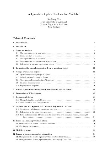
A Quantum Optics Toolbox for Matlab 5Sze Meng TanThe University of AucklandPrivate Bag 92019, AucklandNew ZealandTable of Contents1 Introduction 22 Installation 23 Quantum Objects 33.1 Therepresentationofpurestates ....................................................33.2 Tensorproductofspaces............................................................43.3 Therepresentationofoperators......................................................53.4 Superoperatorsanddensitymatrixequations ..........................................63.5 Calculationofoperatorexpectationvalues ............................................84 Extracting the underlying matrix from a quantum object 105 Arrays of quantum objects 105.6 Operations involving arrays of objects . . . . . . . . . . . . . . . . . . . . . . . . . . . . . . . . . . . . . . . . . . . . . . . 125.7 OrbitalAngularMomentumStates..................................................135.8 SimultaneousDiagonalizationofOperators...........................................145.9 OperatorExponentiation ..........................................................155.10 SuperoperatorAdjoints ............................................................166 Hilbert Space Permutation and Calculation of Partial Traces 167 Truncation of Hilbert space 178 Exponential Series 188.11 ManipulatingExponentialSeries....................................................198.12 TimeEvolutionofaDensityMatrix.................................................219 Correlations and Spectra, the Quantum Regression Theorem 229.13 Twotimecorrelationandcovariancefunctions........................................229.14 Calculationofthepowerspectrum ..................................................239.15 Force and momentum di¤usion of a stationary two-level atom in a standing-wave light…eld .........................................................................2410 Force on a moving two-level atom 2610.16IntroductiontoMatrixContinuedFractions ..........................................2610.17Settinguptheproblem ............................................................2911 Multilevel atoms 3112 Larger problems, numerical integration 3412.18Integration of a master equation with a constant Liouvillian . . . . . . . . . . . . . . . . . . . . . . . . . . . . 3612.19Integration of a master equation with a time-varying Liouvillian . . . . . . . . . . . . . . . . . . . . . . . . 37

A Quantum Optics Toolbox for Matlab 5 213 Quantum Monte Carlo simulation 3813.20Individualtrajectories .............................................................3913.21Computingaverages...............................................................4114 Quantum State Di¤usion 4315 Quantum-state mapping between atoms and …elds 4416 Quantum Computation Functions 4517 Disclaimer 4618 References 46

A Quantum Optics Toolbox for Matlab 5 3IntroductionIn quantum optics, it is often necessary to simulate the equations of motion of a system coupled toa reservoir. Using a Schrödinger picture approach, this can be done either by integrating the masterequation for the density matrix[1] or by using some state-vector based approach such as the quantumMonte Carlo technique[2][3]. Starting from the Hamiltonian of the system and the coupling to the baths,it is in principle a simple process to derive either the master equation or the stochastic Schrödingerequation. In practice, however for all but the simplest systems, this process is tedious and can be errorprone.For a system which is described by an n dimensional Hilbert space, there are n simultaneouscomplex-valued Schrödinger equations of motion and n 2 simultaneous real-valued equations of motionfor the components of the Hermitian density matrix. Although the matrix of coe¢cients is the squareof the number of simultaneous equations (i.e. n 2 for the Schrödinger equation and n 4 for the densitymatrix equations), many of these coe¢cients are zero and it is feasible to integrate systems of 10 2 to 10 3equations numerically.The recent interest in quantum systems involving only a few photons and atoms in cavity QED systemsand in quantum logic devices makes it often possible to employ a truncated Fock space basis for the light…eld modes, yielding essentially exact numerical simulations. This document addresses the problem ofsemi-automatically generating the equations of motion for a wide variety of quantum optical systemsworking directly from the Hamiltonian and couplings to the bath. This approach substantially reducesthe algebraic manipulations required, allowing a variety of con…gurations to be investigated rapidly.The Matlab programming language[4] is used to set up the equations of motion. Matlab supportsthe manipulation of complex valued matrices as primitive data objects. This is particularly convenientfor representing quantum mechanical operators taken with respect to some basis. We shall see that thesparse matrix facilities built into the Matlab language allow e¢cient computation with these quantities.Once the equations of motion have been derived, a variety of solution techniques may be employed. Forsmall problems with constant Liouvillians for which the eigenvectors and eigenvalues may be computedexplicitly, the steady-state and time-dependent solutions of the master equation can be found in formswhich may be evaluated at arbitrary times without step-by-step numerical integration. For Liouvillianswith special time-dependences, techniques such as matrix continued fractions may be used to …nd periodicsolutions of the master equation which are useful in problems such as calculating the forces on atoms instanding light …elds. When direct numerical integration cannot be avoided due to the size of the statespace or non-trivial time-dependence in the Hamiltonian, a selection of numerical di¤erential equationsolvers written in C may be used to carry out the solution after the problem has been formulated inMatlab.In the next section, the overall philosophy of the toolbox is described and the basic “quantum object”data structures are introduced. Quantum objects are generic containers for scalars, states, operators andsuperoperators and thus possess a fairly rich structure. This will be elaborated upon and illustratedthrough a series of problems which demonstrate how the toolbox may be used.InstallationTo install the toolbox on an IBM compatible PC running Windows, unpack the …les into some convenientdirectory, such as c:nqotoolbox. The executable …les _solvemc.exe, _stochsim.exe and_solvesde.exe and the associated batch …les solvemc.bat, stochsim.bat and solvesde.bat whichare in the bin subdirectory must be copied to a directory which is on the system path (set up in the autoexec.bat…le, and which is usually distinct from the Matlab path). Unless this is done, the numericalintegration routines will not operate correctly.On a machine running Unix or other operating system, it is necessary to make the executable …lessolvemc; stochsim and solvesde from the …les contained within subdirectories of the unixsrc directory.Simply compile and link all the C …les contained in each of the subdirectories to produce the appropriateexecutable …les and ensure that these executables are placed in a directory on the path. For example,if /home/mydir/bin is on the path, in order to compile solvemc using the Gnu C compiler, one shouldchange to the subdirectory unixsrc/solvemc and issue a command such asgcc -o /home/mydir/bin/solvemc *.c -lmAfter starting Matlab, add the directory containing the toolbox to the path by entering a commandsuch as addpath(’c:/qotoolbox’). It should now be possible to access the toolbox …les. In order to try

A Quantum Optics Toolbox for Matlab 5 4out the examples, one should addpath(’c:/qotoolbox/examples’) as well. If you wish these directoriesto be added to your Matlab path automatically, it will be necessary to use a startup.m …le, or to editthe system-wide default path in the matlab/toolbox/local directory.Run the script qdemos to view a series of demonstrations contained within the examples directory.The buttons with an asterisk in the names indicate those demonstrations which require the numericalintegration routines to be correctly installed. These demonstrations are discussed in more detail in thisdocument, where they are referred to in terms of the script …les which run them. In order to show thesescript …le names rather than the descriptions of the routines in the buttons of the demonstration, turnon the checkbox labelled “Show script names”. When running these demonstrations, prompts in thecommand window will lead the user through each example. The menu window will be hidden until whileeach demonstration is in progress.Note that the …les in the examples directory beginning with the letter x are script …les which may alsobe run manually from the command line. Usually the …le xprobyyy calls a function …le named probyyywhich is discussed in the notes.This article is presented as a tutorial and the reader is encouraged to try out the examples if acomputer is available. A reference manual with more complete details of the implementation is currentlyunder preparation. Lines which are in typewriter font and preceeded by a >> may be typed in at theMatlab prompt.Quantum ObjectsWithin the toolbox, the basic data type is a “quantum array” object which, as its name suggests, isa collection of one or more simple “quantum objects”. Each quantum object may represent a vector,operator or super-operator over some Hilbert space representing the state space of the problem. In thecomputer, the members of a quantum array object are represented as complex-valued vectors or matrices.We shall use the terms “element” and “matrix” to refer to the representation of the individual quantumobjects and the terms “member” and “array” to refer to the organization of these objects within aquantum array object.The usual arithmetic operations are overloaded so that quantum array objects may be combinedwhenever this combination makes sense. Furthermore, many of the toolbox functions are polymorphic,so that, for example, if a state is required, this state may be speci…ed either as a ket vector or as a densitymatrix. In the following sections, we shall introduce the structure of a quantum object and show howseveral of these may be collected into an array.1. TherepresentationofpurestatesGiven a single quantum system such as a mode of a quantized light …eld or the internal dynamics of anatom, a state ket can be represented by a column vector whose components give the expansion coe¢cientsof the state with respect to some basis. In Matlab, a column vector with n components is written as[c1;c2;...;cn] where the semicolons separate the rows. In order to create a state within the toolboxand assign it to a variable psi, we would enter a command such as>> psi = qo([0.8;0;0;0.6]);The function qo packages the column vector into as a quantum object. It is technically called aconstructor for the class qo. As a result of the assignment, psi is now a simple quantum object (i.e., aquantum array object with a single member). If one now types psi at the prompt, the response is>> psipsi = Quantum objectHilbert space dimensions [ 4 ] by [ 1 ]0.8000000.6000Within the quantum object, additional information is stored together with the elements of the vector.In the example, this additional information was deduced from the size of the input argument to qo. Moreprecisely, an object of type qo contains the following …elds:

A Quantum Optics Toolbox for Matlab 5 5dims Hilbert space dimensions of each object in the arraysize Size of the array, specifying the number of membersshape Shape of each object in the array as a two-dimensional matrixdata Data for the quantum object stored as a “‡attened” two-dimensional matrixFor the most part, the user need not be too concerned about manipulating these …elds, as they arehandled by the toolbox routines. In order to examine these …elds, one may enter>> psi.dims[4] [1]>> psi.size1 1>> psi.shape4 1>> psi.data(1,1) 0.8000(4,1) 0.6000The user can examine, but not modify the contents of these …elds. The dims …eld is the cell array{[4],[1]}, which means that the objects are matrices of size 4 £ 1; which are column vectors. The size…eld is [1,1] since there is only one object in the array. The shape …eld indicates that each object is ofsize 4£1; which at this stage may appear to duplicate the information in the dims …eld, but the distinctionwill become clearer as we proceed. Finally the data themselves, i.e., the numbers 0.8, 0.0, 0.0 and 0.6,are stored as a single column in the data …eld as a sparse matrix (i.e., only the non-zero elements arestored explicitly). Note that it is also possible to use dims(psi), size(psi) and shape(psi) to accessthe above information.In order to produce a unit ket in an N dimensional Hilbert space, the toolbox function basis(N,indx)creates a quantum object with a single one in the component speci…ed by indx. Thus we have, for example,>> basis(4,2)ans = Quantum objectHilbert space dimensions [ 4 ] by [ 1 ]01002. Tensor product of spacesOften, we are concerned with systems which are composed of two or more subsystems. Suppose thereare two subsystems for which the dimension of the state space for the …rst alone is m andthatofthesecond alone is n: The dimension of the Hilbert space for the composite system is mn. If the …rstsystem is prepared in state c =[c1; :::; cm] and the second system is independently prepared in the stated =[d1; :::; dn], the joint state is given by the tensor product of the states which has components[c1*d1; ... ; c1*dn; c2*d1; ... ; c2*dn; ... ; cm*d1; ... ; cm*dn]Within the toobox, the construction of the tensor product is carried out as shown in the followingexample:>> psi1 = qo([0.6; 0.8]);>> psi2 = qo([0.8; 0.4; 0.2; 0.4]);>> psi = tensor(psi1,psi2)psi = Quantum objectHilbert space dimensions [ 2 4 ] by [ 1 1 ]0.48000.24000.12000.24000.64000.32000.16000.3200

A Quantum Optics Toolbox for Matlab 5 70 0.7071 00.7071 0 0.70710 0.7071 0It is also possible to obtain the operator for ^n ¢ J where n is a three component vector specifying adirection by specifying this vector in place of the type string as the second argument of jmat. The vectorn is normalized to unit length, and the operator returned is ^n x J x +^n y J y +^n z J z :The Pauli spin operators are of special signi…cance since they may be used to represent a two-levelsystem. The convention we use is to de…ne¾ x =µ 0 11 0µ 0 ¡i=2J x (1=2) ;¾ y =i 0µ 1 0=2J y (1=2) ;¾ z =0 ¡1which are obtained by using sigmax, sigmay and sigmaz whileµ µ 0 00 1¾ ¡ =and ¾1 0+ =0 0=2J (1=2)zare generated using sigmam and sigmap. Note that ¾ § = 1 2 (¾ x § i¾ y ) ; which is somewhat inconsistentwith the de…nition J § = J x § iJ y used for the general angular momentum operators.The function tensor described above is useful for constructing operators in a joint space as it is forconstructing states. Consider a speci…c example of a cavity supporting mode a in which a single two-levelatom is placed. If we truncate the space of the light …eld to be N dimensional, the following lines of codede…ne operators which act on the space of the joint system:ida = identity(N); idat = identity(2);a = tensor(destroy(N),idat);sm = tensor(ida,sigmam);In the …rst line, identity operators are de…ned for the space of the light …eld and the space of the atom.The annihilation operator for the light …eld does not a¤ect the space of the atom, and so a is de…nedwith the identity operator in the atomic slot. Similarly the atomic lowering operator sm is de…ned withthe identity in the light …eld slot.Let us consider constructing the Hamiltonian operator for the above system driven by an externalclassical driving …eld.H = ! 0 ¾ + ¾ ¡ + ! c a y a + ig ¡ a y ¾ ¡ ¡ ¾ + a ¢ + E ¡ e ¡i! Lt a y + e i! Lt a ¢where ! 0 is the atomic transition angular frequency, ! c is the cavity resonant angular frequency and ! Lis the angular frequency of the classical driving …eld, and we have taken ~ =1: Movingtoaninteractionpicture rotating at the driving …eld frequency yieldsH =(! 0 ¡ ! L ) ¾ + ¾ ¡ +(! c ¡ ! L ) a y a + ig ¡ a y ¾ ¡ ¡ ¾ + a ¢ + E ¡ a y + a ¢with the Matlab de…nitions given above, the operator H is simply given byH=(w0-wL)*sm’*sm + (wc-wL)*a’*a + i*g*(a’*sm-sm’*a) + E*(a’+a);This can be written down by inspection and will automatically generate the operator for H in thechosen representation. Notice that by de…ning the operators a and sm as above, we can generate therepresentation for operators such as a y ¾ ¡ simply by writing a’*sm. This could alternatively have beenformed using tensor(destroy(N)’,sigmam) but the advantage of the former construction is its similarityto the analytic expression. Since the operators are stored as sparse matrices, the fact that a and smhave dimensions larger than destroy(N)’ and sigmam is not an excessive overhead for the notationalconvenience.4. Superoperators and density matrix equationsThe generic form of a master equation isd½dt = L½

A Quantum Optics Toolbox for Matlab 5 8where ½ is the density matrix and the Liouvillian L is a superoperator which may involve both premultiplicationand postmultiplication by other operators. For example, a typical Liouvillian (for spontaneousemission from a two-level atom) isL½ = °¾ ¡ ½¾ + ¡ ° 2 ¾ +¾ ¡ ½ ¡ ° 2 ½¾ +¾ ¡This is a linear, operator-valued transformation acting on ½: When a super-operator such as L acts on amatrix such as ½; this is actually done by regarding the elements of the matrix ½ as being strung out as acolumn vector. In Matlab, given a matrix such as A=[1,2,3;4,5,6;7,8,9], we can construct the vectordenoted by A(:) which simply consists of the elements of A written column-wise, so that in this example,A(:)=[1;4;7;2;5;8;3;6;9]. We shall follow the convention of column-wise ordering when convertingfrom matrices to vectors and call this process “‡attening” the matrix. Corresponding to a matrix ½, weshall denote the ‡attened vector by e½:Suppose that we have the operator a and the density operator ½ with 2 £ 2 matrix representationsa =µ a11 a 12a 21 a 22µ ½11 ½and ½ = 12:½ 21 ½ 22If we premultiply the matrix ½ by the matrix a; we obtainµ a11 ½a½ = 11 + a 12 ½ 21 a 11 ½ 12 + a 12 ½ 22a 21 ½ 11 + a 22 ½ 21 a 21 ½ 12 + a 22 ½ 22The column vector associated with a½ is related to that associated with ½ via the following linear transformation01 01 0 1a 11 ½ 11 + a 12 ½ 21 a 11 a 12 0 0 ½ 11fa½ = B a 21 ½ 11 + a 22 ½ 21C@ a 11 ½ 12 + a 12 ½ 22A = B a 21 a 22 0 0C B ½ 21C@ 0 0 a 11 a 12A @ ½ 12A =spre(a)~½a 21 ½ 12 + a 22 ½ 22 0 0 a 21 a 22 ½ 22The 4 £ 4 matrix represents the superoperator associated with premultiplication by a: We see that itmay be formed simply from the matrix a: This is true in general, and the function spre in the toolboxis provided in order to compute the superoperator associated with premultiplication by a matrix. Thusif A and B are square matrices of the same size, the ‡attened version of A*B is equal to spre(A)*B(:).In the same way, we may represent postmultiplication by a matrix by a superoperator acting on thevector representation. In the toolbox, the function spost performs this conversion so that the ‡attenedversion of A*B can alternatively be found as spost(B)*A(:). We regard spost(B) as a superoperatoracting on the ‡attened matrix A(:) which is a column vector. Notice that since ‡attening alwaysproduces a column vector, superoperators always act on the left of such vectors, i.e.,eab =spost(b)~a:The advantage of considering superoperators rather than operators is that the actions of premultiplicationand postmultiplication by operators are both converted into premultiplication by a superoperator.For example, the Liouvillian L given aboveL½ = °¾ ¡ ½¾ + ¡ ° 2 ¾ +¾ ¡ ½ ¡ ° 2 ½¾ +¾ ¡ ;may be written as a single superoperator once we have the matrices sm representing ¾ ¡ and sm’ representing¾ + : It is simplygamma*(spre(sm)*spost(sm’)-0.5*spre(sm’*sm)-0.5*spost(sm’*sm))Note that the calculation of ¾ ¡ ½¾ + involves postmultiplication by ¾ + and premultiplication by ¾ ¡ :These operations correspond to the multiplication of the superoperators spre(sm)*spost(sm’) whichhappens to be commutative in this case. In the other two terms, we compute the superoperatorscorresponding to premultiplication and postmultiplication by ¾ + ¾ ¡ : It is also possible to consider aterm such as ¾ + ¾ ¡ ½ as a premultiplication by ¾ ¡ followed by a premultiplication by ¾ + and so thiscould be expressed as spre(sm’)*spre(sm)*rho(:). It is easy to check however that spre(sm’*sm) =spre(sm’)*spre(sm), and that it is more e¢cient to compute this by multiplying the operators together…rst.

A Quantum Optics Toolbox for Matlab 5 9If there is a Hamiltonian component to the evolution as well, represented by the matrix H, wesimplyadd in the commutator to the LiouvillianL H ½ = ¡i [H; ½] =¡i (H½ ¡ ½H)This is written using the toolbox as-i*(spre(H)-spost(H))From these examples, it should be clear that obtaining the sparse matrix representation of the Liouvillianstarting from the Hamiltonian and the collapse operators in the Linblad form of the masterequation is largely automatic, with the bookkeeping done using the sparse matrix structures.In the toolbox, an additional re…nement has been included. When the functions spre and spostare applied to operators, they return structures which are more complex than just matrices and so it ispossible to identify the resulting objects as superoperators. For example, if we enter>> a = tensor(destroy(5),identity(2))a = Quantum objectHilbert space dimensions [ 5 2 ] by [ 5 2 ]...>> L = spre(a)L = Quantum objectHilbert space dimensions ([ 5 2 ] by [ 5 2 ]) by ([ 5 2 ] by [ 5 2 ])...we …nd here that a is an operator with Hilbert space dimensions [5 2] by [5 2] since it acts onten-dimensional kets to produce ten-dimensional kets. Once we use the function spre, the dimensions become([ 5 2 ] by [ 5 2 ]) by ([ 5 2 ] by [ 5 2 ])which indicates that L is now a super-operatorwhich acts on matrices of dimensions [5 2] by [5 2] to produce a matrix of the same dimensions. Thuswe may write L*rho to compute the product of an super-operator and a density matrix (operator),returning a matrix (operator) result. Internally, the toolbox calculates the product by usingreshape(L*rho(:),N,N)where the colon operator and the reshape command are used to ‡atten the density matrix and “un-‡atten” the resulting vector. It should be emphasized that one should not use the reshape commandexplicitly with toolbox objects, as this is done automatically. This is an example of operator overloadingsince the * operator carries out multiplication of super-operators and operators or of two operatorsdepending on what makes sense.5. Calculation of operator expectation valuesGiven the density matrix ½;…nding the expectation value of some operator a involves calculation ofhai =Tr(a½) ;which is a linear functional acting on ½ to produce a number.expectation value of a is given bySimilarly, given a state ket jÃi ; thehai =Tr(a jÃihÃj) =hÃj a jÃiIn the toolbox, the function expect(op,state) is used to compute the expectation value of an operatorfor the speci…ed state. The state may be speci…ed either as a density matrix or as a state vector. Notethat the trace of ½ may be found by setting a to the identity.Steady state solution of a Master EquationThis is a simple, yet complete example of a problem which may be solved using the toolbox. Weconsider a cavity with resonant frequency ! c and leakage rate · containing a two-level atom with transitionfrequency ! 0 , …eld coupling strength g and spontaneous emission rate °: Thecavityisdrivenbyacoherent(classical) …eld E which is such that the maximum photon number in the cavity is small so that it isadequate to represent it by a truncated Fock state basis. The Hamiltonian of the system is as givenabove,H =(! 0 ¡ ! L ) ¾ + ¾ ¡ +(! c ¡ ! L ) a y a + ig ¡ a y ¾ ¡ ¡ ¾ + a ¢ + E ¡ a y + a ¢

A Quantum Optics Toolbox for Matlab 5 10and there are two collapse operatorsC 1 = p 2·aC 2 = p °¾ ¡corresponding to leakage from the cavity and spontaneous emission from the atom respectively.Liouvillian has the standard Linblad formL = 1 2Xi (H½ ¡ ½H)+ C k ½C y k ¡ 1 ³´C y k2C k½ + ½C y k C k :k=1Having found the Liouvillian, we seek a steady-state solution for ½, i.e., we wish to …nd ½ such thatL½ =0: The toolbox function steady(L) returns the density matrix ½ representing the steady-statedensity matrix for an arbitrary Liouvillian L: This is done using the inverse power method for obtainingthe eigenvector belonging to eigenvalue zero. The solution is normalized so that Tr (½) =1:D EAs an illustration, the function below returns the steady-state photocounting rates C y 1 C 1 andD EC y 2 C 2 for photodetectors monitoring the output …eld of the cavity and the spontaneous emission of theatom,aswellashai which is proportional to the intracavity …eld. The intracavity photon number canbe found from ­ a y a ® E=DC y 1 C 1= (2·) and it is also easy to add to the programme to …nd expectationvalues of other quantities such as ¾ z or higher moments moments of the intracavity …eld a:function [count1, count2, infield] = probss(E,kappa,gamma,g,wc,w0,wl,N)%% [count1, count2, infield] = probss(E,kappa,gamma,g,wc,w0,wl)% solves the problem of a coherently driven cavity with a two-level atom%% E = amplitude of driving field, kappa = mirror coupling,% gamma = spontaneous emission rate, g = atom-field coupling,% wc = cavity frequency, w0 = atomic frequency, wl = driving field frequency,% N = size of Hilbert space for intracavity field (zero to N-1 photons)%% count1 = photocount rate of light leaking out of cavity% count2 = spontaneous emission rate% infield = intracavity fieldida = identity(N); idatom = identity(2);% Define cavity field and atomic operatorsa = tensor(destroy(N),idatom);sm = tensor(ida,sigmam);% HamiltonianH = (w0-wl)*sm’*sm + (wc-wl)*a’*a + i*g*(a’*sm - sm’*a) + E*(a’+a);% Collapse operatorsC1 = sqrt(2*kappa)*a;C2 = sqrt(gamma)*sm;C1dC1 = C1’*C1;C2dC2 = C2’*C2;% Calculate the LiouvillianLH = -i * (spre(H) - spost(H));L1 = spre(C1)*spost(C1’)-0.5*spre(C1dC1)-0.5*spost(C1dC1);L2 = spre(C2)*spost(C2’)-0.5*spre(C2dC2)-0.5*spost(C2dC2);L = LH+L1+L2;% Find steady staterhoss = steady(L);% Calculate expectation valuescount1 = expect(C1dC1,rhoss);count2 = expect(C2dC2,rhoss);The

A Quantum Optics Toolbox for Matlab 5 11infield = expect(a,rhoss);A driver routine called xprobss demonstrates how we can obtain the system response as the frequencyof the driving …eld is swept across the common resonant frequencies of the atom and cavity. Figures 1and 2 show the results of this calculation. In Figure 2 it is evident that the e¤ect of the atom on thecavity response is reduced for the stronger driving …eld.0.25Photocount rates0.200.150.100.05κ = 2γ = 0.2g = 1E = 0.50.00-6 -4 -2 0 2 4 6Detuning between driving field and cavityFigure 1: Photocounting rates for cavity output light (solid line) and for atomic spontaneous emission(dashed line)Although the separation of the problem into a function which computes the response for a givenset of parameters and a driver routine which loops over the parameter values is convenient, it leads toseveral redundant re-evaluations of quantities such as L1 and L2 which are not changed as the drivingfrequency is swept. The example …le xprobss2.m illustrates a more e¢cient way of carrying out theabove calculation.Extracting the underlying matrix from a quantum objectGiven a quantum object, the underlying matrix can be extracted by using subscript notation. Forexample,>> A = qo([1,2,0;2,0,6;3,0,9])A = Quantum objectHilbert space dimensions [ 3 ] by [ 3 ]1 2 02 0 63 0 9>> A(:,:)ans =(1,1) 1(2,1) 2(3,1) 3(1,2) 2(2,3) 6(3,3) 9Notice that only the non-zero elements of A are stored as a sparse matrix. This may be converted intoa full matrix using the notation full(A(:,:)).Instead of using the colon notation which extracts all the rows and/or columns of the matrix, one canprovide an integer vector of indices using the standard Matlab rules. Thus for example, with the above

A Quantum Optics Toolbox for Matlab 5 12-20-40E = 0.5E = 0.1Phase shift (degrees)-60-80-100-120-140-160κ = 2γ = 0.2g = 1-6 -4 -2 0 2 4 6Detuning between driving field and cavityFigure 2:Phase of intracavity light …eld for two values of external driving …eld amplitudede…nition of A,>> full(A(2:3,[1,3]))ans =2 63 9Note that the result of a subscripting operation applied to a quantum object is to produce an ordinarysparse matrix, not a quantum object.Arrays of quantum objectsSo far, we have created single quantum objects which may be thought of as quantum array objects witha single member. It is sometimes convenient to construct an array of several quantum objects, all withthe same dimensions. For example, the state vector of an electron con…ned in one dimension is a spinorvaluedfunction, so that at each point in space, there is a 2 £ 1 ket. If space is discretized, we have a ketat each of a set of N points. This can be conveniently represented by a N £ 1 member array of quantumobjects each of dimensions 2 £ 1: As another example, we may wish to consider the three operators J x ;J y and J z together as a 3 £ 1 array of operators which we may denote by J.Consider entering the array of angular momentum operators associated with j =2: This may be doneas follows:>> J = [jmat(2,’x’); jmat(2,’y’); jmat(2,’z’)]J = 3 x 1 array of quantum objectsHilbert space dimensions [ 5 ] by [ 5 ]Member (1,1)...Member (2,1)...Member (3,1)...The size …eld of this object is [3,1] indicating the number of members in the array. It is possibleto access the members by using subscipts within braces. Thus for example, J{2} or J{2,1} evaluates. One can also assign to a member of a quantum object array by placing asubscripted expression on the left of the equals sign, so that we could alternatively have written>> J = jmat(2,’x’); % J is a quantum array object with a single member>> J{2} = jmat(2,’y’); % Define second memberto the second member J (2)y

A Quantum Optics Toolbox for Matlab 5 13>> J{3} = jmat(2,’z’); % Define third memberThis makes J into a 1 £ 3 quantum array object. Note that it is important that J is a quantum arrayobject before additional members are assigned to it. If necessary, a null qo object may be generated …rstas illustrated below>> J = qo; % Define a null object>> J{1} = jmat(2,’x’); % Define first member>> J{2} = jmat(2,’y’); % Define second member>> J{3} = jmat(2,’z’); % Define third memberIf the initial call to the constructor is omitted, J becomes a cell array of simple quantum objects,rather than a single quantum array object with three members.The arrays of quantum objects can have as many dimensions as desired. For example, one can makean assignment to J{2,2}, which would automatically enlarge the array to the smallest size which includesall the assigned members, leaving the unassigned members equal to zero. Subscripting with index vectorsand the colon operator are also supported. Note however that the special index end may not be used.In the above, the construction [A;B;C] was used to form a column of objects. It is similarly possibleto constuct a row of objects by using [A,B,C] or alternatively [A B C]. The rules for constructing arraysare identical to those for making Matlab matrices and so arrays may also be concatenated horizontally orvertically in the usual way. Arrays with more than two dimensions can also be constructed by assigningto an element with more than two subscripts, but support for such constructs is still rudimentary. Inparticular, the cat function has not been implemented.The function jmat may also be called with only one argument j, in which case it returns the 3 £ 1array, formed manually above. Similarly, basis described previously may also be called with a singleargument, e.g., basis(N) in which case it returns an 1 £ N array of quantum objects, the k’th memberbeingaunitketwithaoneinthek’th element of the matrix.6. Operations involving arrays of objectsThe basic operations which are de…ned on individual quantum objects may also be applied to arraysof objects. Unary operations, such as the transpose (.’) and conjugate transpose (’) operationswhenapplied to an array of quantum objects cause the operation to be applied to each member of the arrayin turn, without changing the shape of the array. Thus for example, if psi is a 3 £ 2 array of kets withHilbert space dimensions [5] by [1]; psi’ is a 3 £ 2 array of bras with Hilbert space dimensions [1] by [5]:Binary operations can be performed on compatible arrays. Two arrays of quantum objects are compatibleif they are of the same size, or if one of the arrays has only one member. When the arrays areof the same size, the binary operations are applied to the corresponding members. For example if wehave a 2 £ 2 array of operators [A B;C D] and a 2 £ 2 array of kets [va vb;vc vd] which have the sameHilbert space dimensions as the operators, the result of multiplying these two arrays is to form the array[A*va B*vb;C*vc D*vd]. If one of the arrays has only one member, that member is applied (using thebinary operation) to each of the elements of the other array and the resulting array has the size of thebigger array. Thus for example, v + [u1;u2;u3] is equal to [v+u1;v+u2;v+u3].Binary operations can often also be performed between quantum object arrays and ordinary double(possibly complex-valued) arrays. If the arrays are of the same size, operations take place betweencorresponding members. For example if [A B;C D] is an array of quantum objects, we can compute [AB;C D]^[3 4;2 5] which evaluates to [A^3 B^4;C^2 D^5]. If one of the arrays has only one member,that member is applied to each of the elements of the other array, and the resulting array has the size ofthe bigger array. Thus for example, 2*[A B;C D]=[2*A 2*B;2*C 2*D].Quantum array objects whose elements are from a one dimensional Hilbert space are regarded asbeing equivalent to ordinary double arrays for the purpose of the above compatibility rules.Table 1 is a list of the operations available for quantum object arrays. Capital letters denote quantumobject (arrays) and lower case letters indicate ordinary double matrices.For all of the above, the array structure of the quantum object is largely ignored as operations takeplace between corresponding members or between a single object and each of an array of objects.The two functions for which the array structure of the objects is important are combine and sum:

A Quantum Optics Toolbox for Matlab 5 16J1sq = sum(J1^2); % or use combine([1,1,1],J1^2);J2sq = sum(J2^2);Jsqtot = sum(Jtot^2);Jztot = Jtot{3};[states,evalues] = simdiag([Jsqtot,Jztot,J1sq,J2sq]);xform = ket2xfm(states,’inv’)For example, we …nd ¯¯j = 3 2 ;m= ¡ 2® 1 =0:5774¯¯m 1 = 1 2 ;m 2 = ¡1 ® +0:8165 ¯¯m 1 = ¡ 1 2 ;m 2 =0 ® :As a second example of the use of simdiag, we demonstrate the GHZ paradox which strikinglyillustrates the di¤erences in the predictions of quantum mechanics and those of locally realistic theories.Consider three spin 1 2particles, on each of which we may choose to measure either the spin in the xdirectionorinthey direction. Associated with the operator ¾ 1 x ¾2 y ¾3 y ; for example, is a measurement ofthe x component of the spin of the …rst particle and the y component of the spin of the second and thirdparticle. Working in units of ~=2; each measurement yields either 1 or ¡1; and so the product of thethree is also either 1 or ¡1:The GHZ argument considers the following four operators which all commute with each other: A 1 =¾ 1 x¾ 2 y¾ 3 y;A 2 = ¾ 1 y¾ 2 x¾ 3 y;A 3 = ¾ 1 y¾ 2 y¾ 3 x and A 4 = ¾ 1 x¾ 2 x¾ 3 x: Under the assumption of local reality, each ofthe spin operators ¾ 1;2;3x;ywill in principle have well-de…ned values, although they may not be measuredappears twice in thesimultaneously. Classically, the product A 1 A 2 A 3 is equal to A 4 since each ¾ 1;2;3yproduct and (§1) 2 =1: On the other hand, the code in the listing shown below (which is in the …lexghz.m) demonstratesthatwhenA 1 ; :::; A 4 are diagonalized simultaneously, there is an eigenvector forwhich the eigenvalues for A 1 ; :::; A 4 are 1; 1; 1; ¡1: This shows that there is a state for which measurementsof A 1 ;A 2 and A 3 are certain to yield 1 but for which a measurement of A 4 would yield ¡1; which isopposite in sign to the product of the results for the …rst three observables. This program is containedin the …le xghz.sx1 = tensor(sigmax,identity(2),identity(2));sy1 = tensor(sigmay,identity(2),identity(2));sx2 = tensor(identity(2),sigmax,identity(2));sy2 = tensor(identity(2),sigmay,identity(2));sx3 = tensor(identity(2),identity(2),sigmax);sy3 = tensor(identity(2),identity(2),sigmay);op1 = sx1*sy2*sy3;op2 = sy1*sx2*sy3;op3 = sy1*sy2*sx3;op4 = sx1*sx2*sx3;[states,evalues] = simdiag([op1 op2 op3 op4]);evalues(:,1)9. Operator ExponentiationThe toolbox overloads the function expm to allow the exponentiation of operators and superoperators.The following examples demonstrate the use of this function together with several of the functions availablefor visualizing states.Consider the displacement and squeezing operators for a single mode of the electromagnetic …eldde…ned byD (®) =exp ¡ ®a y ¡ ® ¤ a ¢µ 1S (") =exp2 "¤ a 2 ¡ 1 2 "ay2The following program (contained in xsqueeze.m) draws the Wigner and Q functions of a squeezed state.The values of ® and " should be chosen to be small enough that the state can be represented adequately

A Quantum Optics Toolbox for Matlab 5 17in a 20 dimensional Fock space. The Wigner and Q functions are computed using the functions wfuncand qfunc at a set of points de…ned by the vectors xvec and yvec which may be chosen arbitrarily.Note that the relationships between x; y and a; a y are assumed to be given bya = g 2 (x + iy) ;ay = g (x ¡ iy)2where g is a constant which may be used to account for various de…nitions in use. If the parameter g isomitted in the call to wfunc or to qfunc, thevalueg = p 2 is assumed.N = 20;alpha = input(’alpha = ’);epsilon = input(’epsilon = ’);a = destroy(N);D = expm(alpha*a’-alpha’*a);S = expm(0.5*epsilon’*a^2-0.5*epsilon*(a’)^2);psi = D*S*basis(N,1);g = 2;xvec = [-40:40]*5/40; yvec = xvec;W = wfunc(psi,xvec,yvec,g);figure(1); pcolor(xvec,yvec,real(W));shading interp; title(’Wigner function of squeezed state’);Q = qfunc(psi,xvec,yvec,g);figure(2); pcolor(xvec,yvec,real(Q));shading interp; title(’Q function of squeezed state’);Intheabove,thestateforwfunc and for qfunc is speci…ed as a ket psi. It is also valid to use adensity matrix to specify the state. The …le xschcat similarly illustrates the calculation of the Wignerand Q functions of a Schrödinger cat state.The operator exponential is also useful for generating matrices for rotations through …nite angles sincea rotation through Á about the n axis may be written as exp (¡in ¢ JÁ) : This is illustrated in the …lexorbital. The …le rotation is also available for converting between descriptions of a rotation speci…edin various formats (as Euler angles, as an axis and an angle, as a 3 £ 3 orthogonal matrix in SO(3) or asa unitary matrix in SO(2)). As an example, try entering rotateworld([pi/3,pi/4,pi/2],’euler’).The …le xrotateworld shows a spinning globe by making successive calls to rotateworld.10. Superoperator AdjointsGiven a superoperator L which acts on a density matrix ½ via the operationL½ = A½Bwhere A and B are operators, we often wish to compute the “superoperator adjoint” e L which is de…nedso that its action on ½ iseL½ = B y ½A ywhere the dagger denotes the adjoints of the operators. In the toolbox, the function sadjoint(L) maybe used to …nd the superoperator adjoint of a quantum object.Hilbert Space Permutation and Calculation of Partial TracesIt is sometimes desirable to re-order the spaces which are multiplied together in a tensor product. Forexample, if we take the product of three operators such as>> A = tensor(destroy(5),jmat(1/2,’x’),destroy(4));the result of this is to produce a matrix with Hilbert space dimensions [5 2 4] by [5 2 4]: The toolboxfunction permute is provided to change the order of the spaces. For example if we enter>> B = permute(A,[3,1,2])the result is to re-order the spaces in A so that B = tensor(destroy(4),destroy(5),jmat(1/2,’x’)).The function permute may be applied to vectors, operators and super-operators.

A Quantum Optics Toolbox for Matlab 5 18Another operation which is often useful is the calculation of partial traces, usually of density matricesor more generally of any operator. Given a density matrix rho with Hilbert space dimensions[d 1 d 2 ::: d m ] by [d 1 d 2 ::: d m ]; it is possible to trace over any collection of indicies by specifying whichindicies are to remain after the trace is computed. For example, if we want to trace over spaces 2; 3; ...;m ¡ 1 so that only spaces 1 and m remain, the required command is>> ptrace(rho,[1,m]);As an example, consider the density matrix of one of the particles of a Bell pair which may be foundby tracing over the second particle:>> up = basis(2,1); dn = basis(2,2);>> bell = (tensor(up,up) + tensor(dn,dn))/sqrt(2);>> ptrace(bell*bell’,1)ans = Quantum objectHilbert space dimensions [ 2 ] by [ 2 ](1,1) 0.5000(2,2) 0.5000The result is indistinguishable from a statistical mixture of up and down with equal probability. Notethat the …rst argument of ptrace which speci…es the state can be either a density matrix or a ket, sothat it would also be valid to write ptrace(bell,1). In either case, the result of ptrace is to producea (reduced) density matrix.On the other hand, suppose that we measure the second particle and …nd it to be in a state which isjà r i =(jupi + jdni) = p 2; we can calculate the probability that this occurs and the conditional state ofthe …rst particle given this measurement result.>> left = (up + dn)/sqrt(2);>> Omega_left = tensor(identity(2),left*left’);>> rho_new = ptrace(Omega_left*bell,1);>> Prob = trace(rho_new);>> rho = rho_new / Probrho = Quantum objectHilbert space dimensions [ 2 ] by [ 2 ](1,1) 0.5000(2,1) 0.5000(1,2) 0.5000(2,2) 0.5000We …nd the value of Prob is 1 2and that the conditional density matrix is just left*left’, indicatingthat the …rst particle is projected into the left state. Computation of trace(rho^2) con…rms that thesystem is left in a pure state. The script xptrace carries out the calculations described above.Truncation of Hilbert spaceGiven an n dimensional Hilbert space, it is sometimes necessary to extract the components of a quantumobject which lie in some m dimensional subspace of the full space. The toolbox function truncate isused to achieve this. First consider an example in which the Hilbert space which is not the tensor productof other spaces:>> A = qo([ 1, 2, 3, 4;5, 6, 7, 8;9,10,11,12;13,14,15,16]);>> B = truncate(A,{[1,2,4]})ans = Quantum objectHilbert space dimensions [ 3 ] by [ 3 ]1 2 45 6 813 14 16The second argument to truncate is a Matlab cell array object (enclosed in braces). This cell array hasonly one element, the selection vector [1,2,4] which speci…es the dimensions along which the truncated

A Quantum Optics Toolbox for Matlab 5 19object is to be computed. The result of the function is another quantum object which is de…ned over athree dimensional Hilbert space. The order of the elements in the selection vector need not be increasing.This allows one to permute the order of the basis elements in the Hilbert space.Next consider a Hilbert space which is the tensor product of several spaces. In this case, the secondargument to truncate is a cell array with as many selection vectors as there are subspaces in the tensorproduct. For example,>> A = tensor(qo(randn(4,4)),qo(randn(3,3)),qo(randn(4,4)))A = Quantum objectHilbert space dimensions [ 4 3 4 ] by [ 4 3 4 ]...>> B = truncate(A,{1:3,[1,3],3:4})B = Quantum objectHilbert space dimensions [ 3 2 2 ] by [ 3 2 2 ]...The truncated operator is de…ned in the space formed by taking the …rst three dimensions of the …rstfour-dimensional subspace, the …rst and third dimensions of the second three-dimensional subspace, andthe last two dimensions of the third four-dimensional subspace. The resulting Hilbert space is twelvedimensional and is the product of subspaces of dimensions 3; 2 and 2 as indicated.If the truncated Hilbert space cannot be expressed as a tensor product of truncated subspaces, it ispossible to specify an arbitrary collection of basis vectors along which the result is to be computed. Forexample, suppose that out of the 48 dimensional Hilbert space over which A operates, we wish to select athree-dimensional subspace. The basis vectors of the full Hilbert space are outer products of three basisvectors, one in the …rst four-dimensional subspace spanned by fu i g 4 i=1, say; one in the second threedimensionalsubspace spanned by fv j g 3 j=1; say; and one in the third four-dimensional subspace spannedby fw k g 4 k=1. Thus for example, we may specify a basis vector of the Hilbert space by the index vector[1,3,2] which represents u 1 ­v 3 ­w 2 : Similarly, the index vectors [1,1,2] represents u 1 ­v 1 ­w 2 and[1,2,4] represents u 1 ­ v 2 ­ w 4 If we wish to truncate A to the space spanned by these three vectors,we use>> B = truncate(A,[1,3,2; 1,1,2; 1,2,4])B = Quantum objectHilbert space dimensions [ 3 ] by [ 3 ]...The second argument to truncate in this case is an ordinary matrix, and not a cell array. The rowsof the matrix specify the indices of the basis vectors in each of the subspaces. The number of rows in thematrix gives the dimensionality m of the truncated space.Note: The truncate function may be applied to bras, kets, operators or superoperators. It also operateselement by element on arrays of quantum objects.Exponential SeriesIn this section we consider obtaining the time-dependent solution of the problem involving an atom in anoptical cavity. In this case, the Liouvillian is time-independent and is small enough to be diagonalizednumerically. Under such circumstances, provided that the eigenvalues of L are not degenerate, it ispossible to write down the time-dependent solution ½ (t) of the master equation as a sum of complexexponentials exp (s j t) where each s j is an eigenvalue of L: Obtaining the solution in this form allows itto be evaluated readily at any time in the future. By contrast, carrying out a numerical integration ofthe master equation can be computationally intensive for large times. In terms of the framework usedin the toolbox, we wish to express the operator ½ (t) as a linear combination of the exp (s j t), wheretheamplitudes may be quantum objects. The general form of this expansion is~½ i (t) = X ja ij exp s j twhere ~½ represents the density operator “‡attened” into a vector. In order to …nd the coe¢cient matrix

A Quantum Optics Toolbox for Matlab 5 20a ij ; we diagonalize L writing it asL ik = X jV ij s j¡ V¡1 ¢ jkThus¡ eLt ¢ ik = X jV ij exp (s j t) ¡ V ¡1¢ jkand so~½ i (t) = X k¡ eLt ¢ ik ~½ k (0) = X jÃX ¡V ij V¡1 ¢ !jk ~½ k (0) exp (s j t)k= X jV ij r j exp (s j t)where r j are the components of the vector r = V ¡1 ~½ (0) : This shows that the matrix A =(a ij )can becomputed by multiplying V by the diagonal matrix with r j on the diagonal. The conversion from L and½ (0) to A and s (the vector of eigenvalues s j of L) is carried out by the toolbox functionES = ode2es(L,r0)which is so-named as it solves a system of ordinary di¤erential equations with constant coe¢cients as anexponential series. In this context, an exponential series is a sum of the forma(t) = X ja j exp (s j t)where each a j is a simple quantum object (i.e., a scalar, vector, operator or superoperator). Once thesolution in the form of an exponential series, the toolbox may be used to evaluate and manipulate suchexponential series, as will be described in more detail in the next section.11. Manipulating Exponential SeriesIn the toolbox, an exponential series is an instance of the class eseries which internally consists of aone-dimensional quantum array object containing the amplitudes and a vector of rates associated withthe series. If we wish to de…ne the scalar exponential seriesf (t) =1+4cost ¡ 6sin2t =1+2exp(it)+2exp(¡it)+3i exp (2it) ¡ 3i exp (¡2it) ;which consists of four amplitudes ( 1; 2; 2; 3i and ¡3i) and four rates ( 0; i;¡i; 2i and ¡2i), theconstructor function for the eseries class may be used as>> f = eseries(1)+eseries(2,i)+eseries(2,-i)+eseries(3i,2i)+eseries(-3i,-2i);Note that the …rst argument to eseries is converted to a quantum object and speci…es an amplitude,while the second is a rate. If the rate is omitted, a rate of zero is assumed. If we wanted to specify anoperator-valued exponential series such asb (t) =¾ x exp (¡2t)+¾ y exp (¡3t)we would have used>> b = eseries(sigmax,-2)+eseries(sigmay,-3);An alternative way of specifying the series is give all the amplitudes as a quantum array object followedby the rates, i.e.,>> b = eseries([sigmax,sigmay],[-2,-3]);but of course, with this method it is not possible to replace the quantum array object by a doublearray. When the exponential series is displayed, the result isb =Exponential series: 2 terms.Hilbert space dimensions [ 2 ] by [ 2 ].Exponent{1} = (-2)

A Quantum Optics Toolbox for Matlab 5 210 11 0Exponent{2} = (-3)0 0 - 1.0000i0 + 1.0000i 0Once an exponential series has been formed, the …eld name ampl maybeusedtoextractthequantumarray object containing the amplitudes and rates maybeusedtoextractthearrayofrates.Thus,>> b.amplans = 2 x 1 array of quantum objectsHilbert space dimensions [ 2 ] by [ 2 ]Member (1,1)0 11 0Member (2,1)0 0 - 1.0000i0 + 1.0000i 0>> b.ratesans=-2-3In the exponential series for b (t), the …rst term is ¾ x exp (¡2t) while the second is ¾ y exp (¡3t) : Onecan place an index in braces to select out some of the terms of the series. Thus we …nd>> b{2}b{2}ans =Exponential series: 1 terms.Hilbert space dimensions [ 2 ] by [ 2 ].Exponent{1} = (-3)0 0 - 1.0000i0 + 1.0000i 0Similarly, b{[2,1]} is the original series with the terms reversed. It is also possible to extract outterms from an exponential series on the basis of the rates. In this case, parentheses are used to carry outthe indexing. Since the rate associated with ¾ x exp (¡2t) in the exponential series b (t) is ¡2; we …ndthat>> b(-2)ans =Exponential series: 1 terms.Hilbert space dimensions [ 2 ] by [ 2 ].Exponent{1} = (-2)0 11 0If the speci…ed rate(s) do not appear within the series, the result is zero. The above constructs maybe combined to extract the amplitude(s) or rate(s) associated with term(s) in the exponential series. Forexample, in order to get the amplitude of the term with rate ¡3; we write>> b(-3).amplans = Quantum objectHilbert space dimensions [ 2 ] by [ 2 ]0 0 - 1.0000i0 + 1.0000i 0The operators listed in Table 2 have been overloaded for exponential series:When using expect for exponential series, either the operator or the state (or both) can be exponentialseries. An operand which is not an exponential series is …rst converted into one (with rate zero) before

A Quantum Optics Toolbox for Matlab 5 22+ Addition, unary plus- Subtraction, unary minus¤ Multiplication’ Conjugate transpose.’ Transposespre(Op)Convert operator to superoperator for premultiplicationspost(Op) Convert operator to superoperator for postmultiplicationexpect(Op,State) Calculate expectation value of an operator for a given stateTable 2:Operations on exponential seriesit is used. It is thus invalid to pass a quantum array object with more than one member as a parameterto expect when the other parameter is an exponential series.Two special functions associated with exponential series are² estidy(ES) which “tidies up” an exponential series by removing terms with very small amplitudesand merging terms with rates which are very close to each other. Control over the tolerancesused to discard and merge terms is available by using additional parameters to estidy. Manyof the functions which manipulate exponential series automatically call estidy(ES) during theiroperation, but the function is also available to the user.² esval(ES,tarray)which evealuates the exponential series ES at the times in tarray. The functionreturns an array of quantum objects of the same size as tarray. In the special case of a scalarexponential series, the result of esval is an array of doubles, rather than an array of quantumobjects. For example, for the exponential series f de…ned above, we may plot f by using>> t = linspace(0,10,101);>> y = esval(f,t);>> plot(t,y);12. Time Evolution of a Density MatrixUsing these techniques, it easy Dto alter the Ecode D for the problem E of an atom in a cavity to give thetime-varying expectation values C y 1 (t) C 1 (t) ; C y 2 (t) C 2 (t) and ha (t)i for a given initial state. If forexample the atom is initially in the ground state and the intracavity light …eld is in the vacuum state,the initial state vector psi0 is the tensor product of basis(N,1) for the light and basis(2,2) for theatom. The initial density matrix is the outer product of the state vector and its conjugate. This …le andits driver are called probevolve and xprobevolve.function [count1, count2, infield] = probevolve(E,kappa,gamma,g,wc,w0,wl,N,tlist)%% [count1, count2, infield] = probevolve(E,kappa,gamma,g,wc,w0,wl,tlist)% solves the problem of a coherently driven cavity with a two-level atom% with the atom initially in the ground state and no photons in the cavity%% E = amplitude of driving field, kappa = mirror coupling,% gamma = spontaneous emission rate, g = atom-field coupling,% wc = cavity frequency, w0 = atomic frequency, wl = driving field frequency,% N = size of Hilbert space for intracavity field (zero to N-1 photons)% tlist = times at which solution is required%% count1 = photocount rate of light leaking out of cavity% count2 = spontaneous emission rate% infield = intracavity field%%% Same code as in probss.m up to line:

A Quantum Optics Toolbox for Matlab 5 23L = LH+L1+L2;% Initial statepsi0 = tensor(basis(N,1),basis(2,2));rho0 = psi0 * psi0’;% Calculate solution as an exponential seriesrhoES = ode2es(L,rho0);% Calculate expectation valuescount1 = esval(expect(C1dC1,rhoES),tlist);count2 = esval(expect(C2dC2,rhoES),tlist);infield = esval(expect(a,rhoES),tlist);Figure 3 shows the photocount outputs from the cavity and the spontaneous emission as functions oftime when the cavity is driven on-resonance. We see that at early times before the atom has had time torespond to the input …eld, the intracavity …eld is high and the spontaneous emission rate is low. As theatom comes to steady-state however, the intracavity …eld strength falls.Photocount rates0.140.120.100.080.060.04Cavity outputSpontaneous emκ = 2γ = 0.2g = 1Atom and cavityon resonance0.020.000 2 4 6 8 10TimeFigure 3:Time-dependent photocount rates for driven cavity with atom.Correlations and Spectra, the Quantum Regression Theorem13. Two time correlation and covariance functionsContinuing with the example of the atom in the cavity with coherent driving, we now turn to thecomputation of the two-time covariance of the intracavity …eld. If we work temporarily in the jointspace of the system and the environment so that the evolution is speci…ed by a total (time-independent)Hamiltonian ^H tot ; the total density matrix evolves according to³½ tot (¿) =exp ¡i ^H´ ³tot ¿ ½ tot (0) exp i ^H´tot ¿ :The time-evolution of the expectation value of an operator such as ^a y is then­ a y (¿) ® ³ ´ ³ ´o=tracena y exp ¡i ^H tot ¿ ½ tot (0) exp i ^H tot ¿where the operator a y (¿) onthelefthandsideisintheHeisenbergpicturewhilethoseontherightarein the Schrödinger picture. If we now wish to …nd the two-time correlation function of the Heisenberg

A Quantum Optics Toolbox for Matlab 5 24operator a (t) ; this may be written in the Schrödinger picture by using the identity­ a y (t + ¿) a (t) ® =trace ¡ a y (t + ¿) a (t) ½ tot (0) ¢³=trace=trace³´exp i ^H tot (t + ¿)n ³a y exp ¡i ^H tot ¿³a y exp´a½ tot (t)exp´¡i ^H tot ¿³i ^H tot ¿³a exp´o:´¡i ^H tot t´½ tot (0)Formally, the right-hand side is identical to that involved in the calculation of ­ a y (¿) ® ; except that theinitial condition ½ tot (0) is replaced by a½ tot (t) : If the operators whose correlation is required are in thespace of the system alone, the integration of the di¤erential equation for time-evolution may be carriedout in the system space alone by utilizing the Liouvillian in place of the total Hamiltonian.This last expression may be interpreted as follows. Starting with initial condition a½ tot (t) ; this ispropagated forward in time using the evolution operator for duration ¿: After this process, the result ispre-multiplied by a y and the trace is computed. If we consider taking the partial trace over the reservoirand re-interpret ½ as the system density operator rather than the total density operator, the evolution intime through ¿ is performed using the exponential of the Liouvillian, i.e., exp (L¿) : This is the essenceof the quantum regression theorem [5]. In the steady-state, as t ! 1; the correlation function dependsonly on ¿: We can thus compute the stationary two-time correlation by1. Setting the initial condition for the di¤erential equation solver to a½ ss where ½ ss is the steady statedensity matrix which is the solution of L½ =0;2. Propagating the initial condition through time ¿; representing the answer as an exponential series,using the function ode2es.3. Finding the trace of a y multiplied by the solution of the di¤erential equation. This can be thought ofas an expectation value with a “state” given by the solution of the di¤erential equation.In view of these considerations, we see that the following code calculates ­ a y (t + ¿) a (t) ® and ­ a y (t + ¿) ;a(t) ®as exponential series in ¿:function [corrES,covES] = probcorr(E,kappa,gamma,g,wc,w0,wl,N)%% [corrES,covES] = probcorr(E,kappa,gamma,g,wc,w0,wl,N)% returns the two-time correlation and covariance of the intracavity% field as exponential series for the problem of a coherently driven% cavity with a two-level atom%% E = amplitude of driving field, kappa = mirror coupling,% gamma = spontaneous emission rate, g = atom-field coupling,% wc = cavity frequency, w0 = atomic frequency, wl = driving field frequency,% N = size of Hilbert space for intracavity field (zero to N-1 photons)%% Same code as in probss up to line:L = LH+L1+L2;% Find steady state density matrix and fieldrhoss = steady(L);ass = expect(a,rhoss);% Initial condition for regression theoremarho = a*rhoss;% Solve differential equation with this initial conditionsolES = ode2es(L,arho);% Find trace(a’ * solution)corrES = expect(a’,solES);% Calculate the covariance by subtracting product of meanscovES = corrES - ass’*ass;­ ® In the last line of this example, the correlation is converted to a covariance by subtracting the constantayhai : This is a scalar which is automatically converted into an exponential series.Figure 4 shows the two-time covariance function for the system for on-resonance driving for two valuesof atom-…eld coupling g. For small values of g; the covariance falls monotonically whereas for larger valuesof g; there are oscillations.

A Quantum Optics Toolbox for Matlab 5 250.0100.0050.000Two-time covariance functionsg = 1κ = 2γ = 0.2Atom and cavityon resonance-0.0050 2 4 6 8 102.0x10 -4 Time1.0x10 -40.0g = 5-1.0x10 -4-2.0x10 -40 2 4 6 8 10Figure 4:Two-time covariance function for di¤erent atom-…eld interaction strengthsThe method described above may similarly used to compute other correlation functions involving twodi¤erent operators, such as ha (t 1 ) b (t 2 )i :14. Calculation of the power spectrumGiven a stationary two-time covariance function Á (¿) = ­ a y (t + ¿) ;a(t) ® expressed as an exponentialseries½ PÁ (¿) =j c j exp(s j ¿) for ¿ ¸ 0Á ¤ (¡¿) for ¿

A Quantum Optics Toolbox for Matlab 5 26Power Spectrum0.011E-31E-41E-5g = 1g = 5κ = 2γ = 0.2Atom and cavityon resonance1E-61E-7-12 -10 -8 -6 -4 -2 0 2 4 6 8 10 12FrequencyFigure 5:Power spectra calculated from two-time covariance functionswhere ¢ is the detuning of the laser relative to the atomic transition. The only dissipative is spontaneousemission with associated collapse operator C 1 = p °¾ ¡ :At any time, if the dipole moment of the atom is d and the electric …eld at the location of the atomis E; the force experienced by the atom in the light …eld is given byf i = @@x i(d x E x + d y E y + d z E z ) :In the case of the one-dimensional standing wave, we …nd thatf = f z = i ((rg ¤ ) ¾ ¡ ¡ (rg) ¾ + )= ¡2ik L g 0 (¾ ¡ ¡ ¾ + )sink L zIn order to …nd the spatial variation of the force when the atom is stationary at z 0 , we simply needto …nd the steady-state values of h¾ + i and h¾ ¡ i : The force on the atom at that position is thenhfi = hf z i = i ((rg ¤ ) h¾ ¡ i¡(rg) h¾ + i) :The momentum di¤usion constant is de…ned as half the rate of increase of the momentum variancewith time, i.e.,D p = 1 d2 dtD(p ¡hpi) 2E :This may simply be related to the force acting on the atom,D p = 1 ¿(p ¡hpi) ¢ d 2dt (p ¡hpi)+ d Àdt (p ¡hpi) ¢ (p ¡hpi) := 1 hf ¢ p + p ¢ fi¡hfi¢hpi2

A Quantum Optics Toolbox for Matlab 5 27At a speci…c time t; assuming that p (¡1) =0;D p (t) = 1 ¿ Z 1f (t) ¢ f (t ¡ ¿) d¿ +20¿Z 1À¡hf (t)i¢ f (t ¡ ¿) d¿=Re=ReZ 10Z 100Z 10Àf (t ¡ ¿) d¿ ¢ f (t)(hf (t) ¢ f (t ¡ ¿)i¡hf (t)i¢hf (t ¡ ¿)i) d¿hf (t) ;f(t ¡ ¿)i d¿where the real part arises because the two-time force correlation function is hermitian symmetric in thetime di¤erence ¿: Thus D p is given by the real part of the time-integral of the force covariance.The methods developed in the previous examples can be applied directly to this problem. Our strategyis to …nd the steady-state density matrix for the atom at the position z 0 and to use this to compute thetwo-time force covariance Á (¿) as an exponential series. Once in the form of an exponential seriesÁ (¿) = X kÁ k exp (s k t)we see that if s k < 0 for all k; theintegralissimplygivenbyZ 10Á (¿) d¿ = ¡ X kThe toolbox function esint(ES) integrates an exponential series from zero to in…nity. This function mayalso be used with extra arguments, esint(ES; t1) integrates a series from t 1 to in…nity and esint(ES; t1; t2)integrates a series from t 1 to t 2 :The …le probstatic.m listed below calculates the force, momentum di¤usion constant and spontaneousemission rate for a stationary atom in a standing wave. The corresponding driver …le is calledxprobstatic.m. Figure 6 shows these quantities for a standing wave with g 0 =1; ¢=2;°=1: Notethat this momentum di¤usion does not include the contribution due to random recoil during spontaneousemission. This additional term is proportional to the spontaneous emission rate and depends on the polarpattern of spontaneous emission.function [force,diffuse,spont] = probstatic(Delta,gamma,g0,kL,z)% [force,diffuse,spont] = probstatic(Delta,gamma,g0,kL,z) calculates the force,% momentum diffusion and spontaneous emission rate for a stationary% two-level atom in a standing wave light field.%% Delta = laser freq - atomic freq% gamma = atomic decay% g0 = coupling between atom and light, g(z) = 2*g0*cos(kL*z)% kL = wavenumber of light% z = position in standing waveg = 2*g0*cos(kL*z);gg = -2*g0*kL*sin(kL*z);%sm = sigmam;%H = -Delta*sm’*sm - i*(g’*sm - sm’*g);F = i*(gg’*sm - gg*sm’);C1 = sqrt(gamma)*sm;%C1dC1 = C1’*C1;LH = -i*(spre(H)-spost(H));L1 = spre(C1)*spost(C1’)-0.5*spre(C1dC1)-0.5*spost(C1dC1);L = LH + L1;Á ks k

A Quantum Optics Toolbox for Matlab 5 28% Find steady state density matrix and forcerhoss = steady(L);force = expect(F,rhoss);spont = expect(C1’*C1,rhoss);% Initial condition for regression theoremFrho = spre(F)*rhoss;% Solve differential equation with this initial conditionsolES = ode2es(L,Frho);% Find trace(F * solES)corrES = expect(F,solES);% Calculate the covariance by subtracting product of meanscovES = corrES-force^2;% Integrate the force covariance and return real partdiffuse = real(esint(covES));21MomentumDiffusionForce0-1-20.60.40.20.0SpontaneousEmission0.30.20.10.0Position in Standing Wave (k Lz)Figure 6: Force, momentum di¤usion and spontaneous emission from a stationary two-level atom in astanding-wave light …eld.Force on a moving two-level atom16. Introduction to Matrix Continued FractionsIn this example, we introduce a problem in which the Liouvillian matrix is time-dependent, so that itis no longer possible to write the answer as a …nite exponential series. If the time-dependence is simplythe sum of a constant and a sinusoidally varying term, it is sometimes possible to use the method ofmatrix continued fractions (see e.g., Risken [7]) in order to obtain special solutions of the equation. Thismethod is especially useful for …nding the force on an atom moving in a light …eld with an intensity orpolarization gradient. We consider a master equation of the formd½dt =(L 0 + L 1 exp (i!t)+L ¡1 exp (¡i!t)) ½and ask for solutions ½ (t) which may be expressed as an exponential series of the form½ (t) =1Xn=¡1½ n exp (in!t) :In the application of …nding the force on a moving atom, the atom is taken to be in…nitely massive and

A Quantum Optics Toolbox for Matlab 5 29is dragged at constant velocity v through a sinusoidally varying light …eld. Since the Hamiltonian (andthe force) depends on the position in the atom, the Liouvillian L contains terms which vary sinusoidallyin space and hence in time with ! = k L v where k L is the wave number of the light …eld. In general, forcertain special values of ! 0 ; there are solutions to the di¤erential equation of the form½ (t) =exp(i! 0 t)1Xn=¡1½ n (! 0 )exp(in!t)We wish to compute the exponential series for the case ! 0 =0; so that ½ (t) is given by a Fourier series.Substituting the supposed solution into the master equation yields1X1Xin!½ n (! 0 )exp(in!t) = (L 0 + L 1 exp (i!t)+L ¡1 exp (¡i!t))n=¡1n=¡1£ ½ n (! 0 )exp(in!t)Equating the coe¢cients of the series yields the tridiagonal recursion relation0=L 1 ½ n¡1 +(L 0 ¡ in!I) ½ n + L ¡1 ½ n+1Such a recursion may often be solved by the method of continued fractions. Suppose that for n ¸ 1; it ispossible to …nd a sequence of matrices S n with the property that ½ n = S n ½ n¡1 : If these matrices exist,then by the recursion relationship, we require[L 1 +(L 0 ¡ in!I) S n + L ¡1 S n+1 S n ] ½ n¡1 =0:ThiscanbedonesimplybysettingorL 1 +(L 0 ¡ in!I) S n + L ¡1 S n+1 S n =0L 1 +[(L 0 ¡ in!I)+L ¡1 S n+1 ] S n =0S n = ¡ [(L 0 ¡ in!I)+L ¡1 S n+1 ] ¡1 L 1 :This expresses S n in terms of S n+1 : We start with some large N and set S N =0: Using this recursionwe obtain the matrix S 1 : This is called a continued fraction because if we consider the case when S andL are in fact a scalars, and if we write a n = ¡L 1 ;b n = L 0 ¡ in!I and c n = L ¡1 ; the recursion may bewritten asand soa nS n =b n + c n S n+1S 1 = c 1 a 2b 1 +b 2 + c 2a 3b 3 + :::which is a classical continued fraction.Similarly, if for n ·¡1; we can …nd a sequence of matrices T n with the property that ½ n = T n ½ n+1 ;we require that[L 1 T n¡1 T n +(L 0 ¡ in!I) T n + L ¡1 ] ½ n+1 =0which can be done by settinga 1from which we …ndL 1 T n¡1 T n +(L 0 ¡ in!I) T n + L ¡1 =0T n = ¡ [(L 0 ¡ in!I)+L 1 T n¡1 ] ¡1 L ¡1 :

A Quantum Optics Toolbox for Matlab 5 30This expresses T n in terms of T n¡1 : We start with some large N and set T ¡N =0: Using this recursionwe obtain the matrix T ¡1 :Having obtained S 1 and T ¡1 ; we return to the tridiagonal relation for n =0; namely0=L 1 ½ ¡1 + L 0 ½ 0 + L ¡1 ½ 1and substitute for ½ 1 and ½ ¡1 in terms of ½ 0 ; obtaining0=(L 1 T ¡1 + L 0 + L ¡1 S 1 ) ½ 0If the matrix L 1 T ¡1 + L 0 + L ¡1 S 1 is singular, which indicates that the choice ! 0 =0does in fact give asolution to the original equation, this enables us to calculate ½ 0 and subsequently ½ n for all other valuesof n; provided that we have stored the appropriate S n and T n :The toolbox function mcfrac uses the matrix continued fraction algorithm to …nd the exponentialseries for the density matrix when given the exponential series for the Liouvillian. This function alsotakes two additional input parameters, one to indicate the value of N at which S N and T ¡N are set tozero in order to start the recursion, and the other to indicate how many terms of the exponential seriesfor ½ are required, since in principle, this is an in…nite series.17. Setting up the problemWe consider a two level atom which is being dragged at constant velocity v through a light …eld whichis oriented along the z direction. Due to the motion, the position of the atom at time t is z = vt: Theelectric …eld experienced by the atom is g(z); normalized such that the interaction energy of the atomwithin the …eld isV (z) =¡ (g ¤ (z) ¾ ¡ + g (z) ¾ + )The force exerted on the atom due to the light …eld isF (z) =(rg ¤ (z) ¾ ¡ + rg (z) ¾ + ) :Since z = vt; each of these becomes a function of time. For a running wave, g(z) is a complex exponentialg (z) =g 0 exp (ik L z) ; whereas for a standing wave, g(z) =2g 0 cos k L z: When using the toolbox, functionswhich are the sum of terms with exponential time-dependence are represented by exponential series. Sofor example, if due to the motion, the atom sees g (t) =2g 0 cos k L vt; this is an exponential series withtwo terms g (t) =g 0 exp (ik L vt)+g 0 exp (¡ik L vt) : In order to specify this using the toolbox, we useg = eseries(g0,i*kL*v) + eseries(g0,-i*kL*v);With this de…nition, the contribution to the Hamiltonian due to the optical potential may be calculatedas an exponential series:A = sigmam;H = -(g’*A + A’*g) + H0;Similarly, the two lines given below compute the exponential series for the force operator:gg = eseries(i*kL*g0,i*kL*v) + eseries(-i*kL*g0,-i*kL*v);F = gg’*A + gg*A’;The Hamiltonian and Liouvillian are also required in the form of exponential series. In the code below,we see that spre(H) and spost(H) convert the operator exponential series for H into superoperator exponentialseries required for the computation of L. Although it is straightforward to manipulate exponentialseries using the toolbox, it is usually best to do as much of the calculation as possible with constant matrices,converting these to exponential series only when absolutely necessary, since calculations involvingseries are somewhat slower than those involving constants. Thus for example, in the typical Liouvillianwith a time-dependent Hamiltonian,L½ = ¡i [H(t);½]+ X nC n ½C y n ¡ 1 2 Cy nC n ½ ¡ 1 2 ½Cy nC n ;the loss terms involving the collapse operators are not time-dependent. We would then calculate thesecollapse operators using ordinary matrices and form the entire superoperatorXC n ½Cn y ¡ 1 2 Cy n C n½ ¡ 1 2 ½Cy n C nn

A Quantum Optics Toolbox for Matlab 5 31as an ordinary matrix (using spre and spost, just as before). Finally, this superoperator would beconverted into an exponential series and combined with the terms involving the Hamiltonian. In the lineL=LH+L1 below, LH is an exponential series while L1 is a quantum object. When they are added together,the result is automatically converted to an exponential series.When the Liouvillian can be expressed as an exponential series of the formL = L 0 + L 1 exp (i!t)+L ¡1 exp (¡i!t) ;(where for this example ! = k L v); there is a special toolbox routinerhoES= mcfrac(LES,Ncf,Nes)which uses the matrix continued fraction method outlined above to …nd the central terms of the exponentialseries for ½; namely if½ =1Xk=¡1½ k exp (ik!t)the routine …nds ½ k for k = ¡Nes; :::; Nes by using Ncf termsofamatrixcontinuedfractionexpansion.Since the force operator and the density matrix are exponential series, the expected value of the force isalso an exponential series. In order to get the correct value for the time-averaged force (i.e., averagedover travel through one cycle of the light), we need the terms ½ 1 and ½ ¡1 for the density matrix, sincethe force operator contains time dependencies of the form exp (§i!t) : More precisely, sinceF (z = vt) =i (rg ¤ (vt) ¾ ¡ ¡rg (vt) ¾ + )= F 1 exp (i!t)+F ¡1 exp (¡i!t) ;the expectation value of F isà 1!XTr (½F )=Tr ½ k exp (ik!t)(F 1 exp (i!t)+F ¡1 exp (¡i!t))=1Xk=¡1k=¡1£ Tr¡½k¡1 F 1¢ +Tr¡½k+1 F ¡1¢¤ exp (ik!t)and the time-averaged force is the term with k =0; namelyTr ¡ ¢½ ¡1 F 1 +Tr(½1 F ¡1 ) :The toolbox function expect has been overloaded to calculate the expectation values when both theoperator and the state are exponential series. The result is also an exponential series. The …le prob2lev.mcalculates the cycle-averaged force on a two-level atom and this is listed below. The Hamiltonian used isH int = ¡¢¾ + ¾ ¡ ¡ (g ¤ (z) ¾ ¡ + g (z) ¾ + )where, as usual ¢ is the laser frequency minus the atomic transition frequency. Notice how the termin the Hamiltonian ¡¢¾ + ¾ ¡ is synthesized using the projection operators onto the excited state, since¾ + ¾ ¡ = jeihej : The result of the calculation is shown in Figure 7 for parameter values corresponding toFigure 1a of Minogin and Serimaa [8]. Taking into account the di¤erence in the notation, the results arein agreement. Note that the result force is an exponential series, and that we require the cycle-averagedterm associated with s =0: This is obtained using the notation force(0).ampl.function force = prob2lev(v,kL,g0,Gamma,Delta)% force = prob2lev(v,kL,g0,Gamma,Delta)%% Calculates the force on a moving two-level atom travelling at% speed v in a standing wave with wavenumber kL. The coupling% strength is g0, the atomic spontaneous emission rate is% Gamma and the detuning is Delta%Ne = 1; Ng = 1; Nat = Ne+Ng;% Form the lowering operator

A Quantum Optics Toolbox for Matlab 5 32A = sigmam;% Time-dependent couplings for atom and fieldg = eseries(g0,i*kL*v) + eseries(g0,-i*kL*v);gg = eseries(i*kL*g0,i*kL*v) + eseries(-i*kL*g0,-i*kL*v);% Form interaction picture Hamiltonian% Excited state termsexcited = basis(Nat,1:Ne);H0 = -Delta*sum(excited*excited’);% Interaction with lightH = -(g’*A + A’*g) + H0;% Force operatorF = gg’*A + gg*A’;% Collapse operatorsC1 = sqrt(Gamma)*A; C1dC1 = C1’*C1;% LiouvilliansL1 = spre(C1)*spost(C1’)-0.5*spre(C1dC1)-0.5*spost(C1dC1);% Calculate total Liouvillian as an exponential seriesLH = -i*(spre(H)-spost(H));L = LH + L1;% Matrix continued fraction calculationrho = mcfrac(L,20,1);force = expect(F,rho);0.6Cycle averaged force on atom0.40.20.0-0.2-0.4kL = 1g = sqrt(25/8)0Γ = 1∆ = -5-0.6-10 -5 0 5 10Velocity in standing waveFigure 7: Cycle-averaged force on a moving two-level atom in a standing wave evaluated using the methodof matrix continued fractions.Multilevel atomsIn this example, we show how the previous calculation for two-level atoms may be straightforwardlyextended to multiple-level atoms in light …elds with polarization gradients, rederiving the results foundby Dalibard and Cohen-Tannoudji [9]. We consider two cases, an atom with a J g =1to J e =2transitionin counter-propagating (¾ + ;¾ ¡ ) light and an atom with a J g = 1 2 to J e = 3 2transition in a light …eldwith counter-propagating lin?lin polarization.With a multilevel atom, the Hilbert space of the atom is of dimension N a = N e +N g where N e =2J e +1and N g =2J g +1: We represent this by a vector whose …rst N e components are the excited state amplitudesfollowed by the N g ground state amplitudes. Since the light …elds are treated classically, this is the full

A Quantum Optics Toolbox for Matlab 5 33Hilbert space. Instead of a single lowering operator ¾ ¡ for the two-level atom, there are three loweringoperators which we shall denote by A ¡1 ;A 0 ; and A 1 which respectively couple to light of ¾ ¡ ;¼and ¾ +polarizations. Each of these involve linear combinations of transitions between excited and ground levels,with weighting factors given by the appropriate Clebsch-Gordon coe¢cients. The matrix representationof one of these matrices of size (N e + N g ) £ (N e + N g ) may be compared with the two-level loweringoperator ¾ ¡ of size 2 £ 2 as followsµe g 0 0 e¾ ¡ =1 0 gµe g 0 0 eA p =a p 0 gwhere a p is a matrix of size N g £ N e containing the Clebsch-Gordon transitions (p =0; §1) and thebold face zeros are block matrices of the appropriate sizes. The toolbox routine murelj calculates thesubmatrices a ¡ ; a 0 and a + for an arbitrary J g to J e transition and the routine murelf calculates thecorresponding matrices for an (F g ;J g ) to (F e ;J e ) transition when the hyper…ne structure induced bynuclear spin I is important.Associated with light …elds travelling in the z direction, there are functions ­ + (z) and ­ ¡ (z) representingthe Rabi frequencies for ¾ + and ¾ ¡ polarizations respectively. The light-induced portion of theinteraction Hamiltonian is given byand the corresponding force operator isH light-atom = ¡ 1 2 (­ + (z) A + + ­ ¡ (z) A ¡ )+h.c.F = 1 2 (r­ + (z) A + + r­ ¡ (z) A ¡ )+h.c.The collapse operators representing spontaneous emission into each of the possible polarizations arep °A¡ ; p °A 0 and p °A + :Let us consider …rst the case of counter-propagating (¾ + ;¾ ¡ )light. The listing below (probmulti1.m)shows how the exponential series for the force may be found. Notice how similar this program is toprob2lev.m for the two-level atom. The noteworthy features are the calculation of the three loweringoperators A p and the formation of the exponential series for the atom-light interaction and the forceoperator. In place of g (and its gradient gg) for the single polarization which interacts with the two levelatom, there are gp and gm (and their gradients ggp and ggm) specifying the amplitudes of the ¾ + and ¾ ¡circular polarizations. For each of the polarizations, there is a travelling wave, the ¾ + light propagatingtowards +z and the ¾ ¡ light propagating towards ¡z: Another noteworthy point is the formation of theloss Liouvillian for all three collapse channels together by using a quantum object array. In Figure 8 thecycle averaged force is shown as a function of the velocity. This is the same as shown in Figure 8 of thepaper by Dalibard and Cohen-Tannoudji [?], taking into account the factor of two which they include intheir units of the force.function force = probmulti1(v,kL,Jg,Je,Omega,Gamma,Delta)% Calculate the force on an atom with light fields in a% sigma+ sigma- configuration.Ne = 2*Je+1; Ng = 2*Jg+1; Nat = Ne+Ng;% Form the lowering operators for various polarizations of light[am,a0,ap] = murelj(Jg,Je);Am = sparse(Nat,Nat); Am(Ne+1:Ne+Ng,1:Ne)=am; Am = qo(Am);A0 = sparse(Nat,Nat); A0(Ne+1:Ne+Ng,1:Ne)=a0; A0 = qo(A0);Ap = sparse(Nat,Nat); Ap(Ne+1:Ne+Ng,1:Ne)=ap; Ap = qo(Ap);% gp = 0.5*Omega*exp(i*kL*z);% gm = 0.5*Omega*exp(-i*kL*z);% ggp = 0.5*i*kL*Omega*exp(i*kL*z);% ggm = -0.5*i*kL*Omega*exp(-i*kL*z);% Due to motion, these become exponential series in time (z=vt)gp = eseries(0.5*Omega,i*kL*v);gm = eseries(0.5*Omega,-i*kL*v);ggp = eseries(0.5*i*kL*Omega,i*kL*v);

A Quantum Optics Toolbox for Matlab 5 340.00Cycle averaged force σ + and σ - beams, Jg=1, Je=20.000-0.01-0.002-0.004Force-0.02-0.03-0.006-0.0080.00 0.01 0.02 0.03 0.04-0.04-0.050.0 0.2 0.4 0.6 0.8 1.0VelocityFigure 8: Cycle averaged force on an atom with a J g =1to J e =2transition in counterpropagating(¾ + ;¾ ¡ ) light …elds. Parameters used are ° =1; ­ =0:25; ¢=¡0:5 and k L =1:ggm = eseries(-0.5*i*kL*Omega,-i*kL*v);% Form interaction picture Hamiltonian% Excited state termsexcited = basis(Nat,1:Ne);H0 = -Delta*sum(excited*excited’);% Interaction with sigma+ lightHp = -(gp’*Ap + gp*Ap’);% Interaction with sigma- lightHm = -(gm’*Am + gm*Am’);%H = H0 + Hp + Hm;% Force operatorFp = (ggp’*Ap + ggp*Ap’);Fm = (ggm’*Am + ggm*Am’);F = Fp + Fm;% Collapse operators as an arrayC = sqrt(Gamma)*[Am,A0,Ap];% Loss LiouvilliansLloss = spre(C)*spost(C’)-0.5*spre(C’*C)-0.5*spost(C’*C);% Calculate total LiouvillianL = -i*(spre(H)-spost(H)) + sum(Lloss);% Matrix continued fraction calculationrho = mcfrac(L,20,1);force = expect(F,rho);The corresponding …le for treating lin?lin polarization are shown in the following listing (probmulti2.m).Note that the changes are limited to the de…nitions of gp and gm (and their gradients ggp and ggm) ofthe light …elds. In Figure 9 the results are shown for this case, using parameters which are the same asin Figure 7 of Dalibard and Cohen-Tannoudji [?].function force = probmulti2(v,kL,Jg,Je,Omega,Gamma,Delta)% Calculate the force on an atom with light fields in a% lin-perp-lin configuration.Ne = 2*Je+1; Ng = 2*Jg+1; Nat = Ne+Ng;% Form the lowering operators for various polarizations of light

A Quantum Optics Toolbox for Matlab 5 35[am,a0,ap] = murelj(Jg,Je);Am = sparse(Nat,Nat); Am(Ne+1:Ne+Ng,1:Ne)=am; Am = qo(Am);A0 = sparse(Nat,Nat); A0(Ne+1:Ne+Ng,1:Ne)=a0; A0 = qo(A0);Ap = sparse(Nat,Nat); Ap(Ne+1:Ne+Ng,1:Ne)=ap; Ap = qo(Ap);% gp = sqrt(0.5)*Omega*sin(kL*z);% gm = sqrt(0.5)*Omega*cos(kL*z);% ggp = sqrt(0.5)*kL*Omega*cos(kL*z);% ggm = -sqrt(0.5)*kL*Omega*sin(kL*z);% Due to motion, these become exponential series in time (z=vt)gp = 0.5*(eseries(sqrt(0.5)*i*Omega,i*kL*v) - eseries(sqrt(0.5)*i*Omega,-i*kL*v));gm = 0.5*(eseries(sqrt(0.5)*Omega,i*kL*v) + eseries(sqrt(0.5)*Omega,-i*kL*v));ggp = 0.5*(-eseries(sqrt(0.5)*kL*Omega,i*kL*v) - eseries(sqrt(0.5)*kL*Omega,-i*kL*v));ggm = 0.5*(eseries(sqrt(0.5)*i*kL*Omega,i*kL*v) - eseries(sqrt(0.5)*i*kL*Omega,-i*kL*v));%% rest of code is identical to probmulti1%0.00Cycle averaged force, lin perp lin, Jg=1/2, Je=3/20.000-0.01-0.005-0.020.00 0.01 0.02 0.03 0.04Force-0.03-0.04-0.050.0 0.2 0.4 0.6 0.8 1.0 1.2 1.4 1.6 1.8 2.0VelocityFigure 9: Cycle-averaged force for an atom with a J g = 1 2 to J e = 3 2con…guration. Parameters are ° =1; ­ =0:3; ¢=¡1; k L =1:transition in a lin?lin light …eldLarger problems, numerical integrationSo far, the problems we have considered have been small enough that it has been possible to carry outoperations such as the diagonalization or the inversion of the Liouvillian matrix. Since the size of theLiouvillian matrix becomes very large as the number of states is increased, these techniques are less usefulfor larger problems. The toolbox thus provides for the numerical integration of the equations of motionfor a variety of problems.1. Even when the Liouvillian matrix L is too large to be inverted or diagonalized (operations whosecomputational load scale with N 3 or N 4 when L is an N £ N matrix), it is often possible to integratethe master equation numericallyd½dt = L½starting with some initial condition ½ (0) = ½ 0 : This is especially the case when L is a sparse matrix,so that the load associated with …nding L½ may be quite small. The strategy we adopt is to exploit

A Quantum Optics Toolbox for Matlab 5 36the techniques used in the toolbox and the sparse matrix algorithms of Matlab to form the matrix Land subsequently to carry out the numerical integration of the equations of motion using a compiledroutine written in C. We use Matlab to write out a …le containing L and ½ 0 which can be read inby the di¤erential equation solver. The solution is written to another …le which may then be readback into Matlab where expectation values and other statistics may be computed. It is also relativelyeasy to treat the case in which the Liouvillian matrix L is explicitly time-dependent, and this is alsoprovided for in the toolbox.2. If there are too many components in the density matrix, an alternative approach is to consider thestate vector à and the Schrödinger equations of motion, which in the case of no dissipation may bewritten in the formi dÃdt = H (t) ÃThis is again an initial value problem, with à (0) = à 0 being given. The routine will compute à at aspeci…ed list of times.3. When dissipation is present, but a wave function approach is still required, it is possible to use aquantum trajectory (or quantum Monte Carlo) approach. In this approach, each trajectory consistsof continuous evolution according to a modi…ed Scrödinger equation of the formi dÃdt = H e¤ (t) Ã;which is punctuated by “quantum jumps” at which the state vector changes discontinuously accordingtoà (t + )= C k (t) à (t ¡ )kC k (t) à (t ¡ )k ;where fC k (t)g are a family of collapse operators, the probability of the kthcollapseinanintervaldtbeing given bykC k (t) à (t)k 2 dt:The e¤ective non-Hermitian Hamiltonian is given byH e¤ (t) =H (t) ¡ i XC y k2(t) C k (t) :kThe above procedure is repeated for a large number of trajectories. For each trajectory, the initialcondition is à (0) = à 0 and the solution takes the form of the stochastic wave function à (t) recordedat a pre-speci…ed list of times together with a classical record which is a list of times at which acollapse occured together with the index of the collapse.4. Since the use of a quantum trajectory approach often requires operator expectation values to beaveraged over many trajectories in order to obtain ensemble predictions, recording the evolution ofthestochasticwavefunctionforeachofthesetrajectoriescanusealargeamountofdiscspace. Inorder to avoid this problem, the quantum trajectories simulation can also be run while specifying a listof operators represented by matrices A k (t) : For each trajectory, the expectation of these operatorsare computed usinghA k (t)i = hà (t) jA k (t) jà (t)ihà (t) jà (t)iThese are averaged over trajectories, and the averaged results are written out after each of a speci…ednumber of trajectories.All of these problems may be solved using a routine called solvemc whichisanexternalprogramspawned as a subprocess from within Matlab. The programme solvemc is written in C using routinesfrom RANLIB[10] and CVODE[11] both available from the Netlib repository. In the PC distribution, the…les _solvemc.exe and solvemc.bat are included, and must be copied to a directory which is on thesystem path. In the Unix distribution, it is necessary to compile and link all the C …les in the subdirectoryunixsrc/solvemc andtoplacetheresultinadirectoryonthepath.

A Quantum Optics Toolbox for Matlab 5 37In the above we have to deal with time-varying operators such as L (t) ;H(t) ;C k (t) and A k (t) :Each of these may be considered as a sparse matrix which depends on time. Typical time-variationsmay include exponential series, which may be of interest when considering atoms moving at constantvelocity in light …elds or for situations with light …elds of several colours. In other cases, we may wish toconsider other time-variations, such as a Gaussian to represent the e¤ects of time-varying light pulses orthe passage of atoms at constant velocity through …elds with spatially varying pro…les. In the toolbox,the standard di¤erential equation solver is designed to represent an operator A (t) as a function serieswhich takes the formA (t) =A 1 f 1 (t)+::: + A n f n (t)where each of A 1 through A n is a sparse matrix, and f 1 through f n are chosen from a library of prede…nedfunctions, each of which may be controlled by several parameters. If A is in fact a constant, only a singleterm in this series is needed and the function f 1 is in fact a constant. In the following examples we shallillustrate the use of the di¤erential equation solver in a variety of problems, and introduce the notationfor forming function series as they become necessary.18. Integration of a master equation with a constant LiouvillianThe solution of ordinary di¤erential equations is handled using the toolbox functions ode2file andodesolve. The former writes out a data …le which contains the de…nition of the problem and the latteris used to spawn the C routine solvemc which reads in the data …le, carries out the numerical integrationand writes the output …le. For a master equation, the output …le will consist of the density matrixevaluated at a list of times. The toolbox function qoread is then used to read in the data as a quantumarray object.A portion of the function probintmaster is shown below in order to illustrate how these routines arecalledinatypicalproblem.% Calculate the Liouvillian L% Initial statepsi0 = tensor(basis(N,1),basis(2,2));rho0 = psi0 * psi0’;% Set up options, if requiredoptions.lmm = ’ADAMS’;options.iter = ’FUNCTIONAL’;options.reltol = 1e-6;options.abstol = 1e-6;% Write out the data fileode2file(’file1.dat’,L,rho0,tlist,options);% Call the equation solverodesolve(’file1.dat’,’file2.dat’);% Read in the output data filefid = fopen(’file2.dat’,’rb’);rho = qoread(fid,dims(rho0),size(tlist));fclose(fid);The problem is set up in the usual way and ode2file is called. The …rst argument to ode2file isthe name of the data …le which is to be generated, here called file1.dat. The second argument is theoperator or super-operator on the right-hand side of the system of di¤erential equations, which in thiscase is just the Liouvillian L. The third argument is the initial condition, which in this case is the densitymatrix rho0 formed by taking the outer product of the initial state psi0. The fourth argument tlist isa vector of times at which the solution is required.The …fth argument to ode2file is optional and is used to specify additional options to the di¤erentialequation integration routines. If present, it is a structure containing one or more of the following …elds:² lmm: A string specifying the linear multistep method used. It may be ’ADAMS’ for the Adams-Bashford method or ’BDF’ for the backwards di¤erence formula. The Adams-Bashford method(which is the default) is preferable for smooth problems, while the backwards di¤erence formulamethod is preferable for sti¤ problems.

A Quantum Optics Toolbox for Matlab 5 38² iter: A string specifying how the implicit problem is solved within each step. It can be ’FUNC-TIONAL’ for functional iteration (the default), or ’NEWTON’ for a Newton method with Jacobipreconditioning. The Newton method is preferable for sti¤ problems.² reltol: A number specifying the relative tolerance, which defaults to 10 ¡6 :² abstol: Either a number or a vector specifying the absolute tolerance, which also defaults to 10 ¡6 :² maxord: Maximum linear multistep model order to be used by solver. Default is 12 for ADAMS and5 for BDF.² mxstep: Maximum number of internal steps to be taken by the solver in its attempt to reach thenext timestep (default 500).² mxhnil: Maximum number of warning messages issued by solver that t + h = t on the next internalstep (default 10).² h0: initial step size.² hmax: maximum absolute value of step size allowed.² hmin: minimum absolute value of step size allowed.Following the call to ode2file, the routine odesolve is called in order to carry out the integration.The two arguments to this routine are the names of the input …le (which should be the same as thatpassed to ode2file) and the name of the output …le, which will be overwritten if it already exisits.Matlab will spawn the external C programme to carry out the integration and waits until the programmeterminates with either a success or failure. This is indicated by the external programme producing one ofthe …les success.qo or failure.qo in the working directory. If the paths have not been set up correctly,the external program will not start and neither of these …les will be produced. In this case, the Matlabprogramme will hang until a break command (usually Control-C) is entered.While the external routine is carrying out the integration, a single-line progress bar indicates how farthe calculation has proceeded. This may either appear in a separate window or in the Matlab commandwindow, depending upon the operating system. On successful completion, the output …le, in this casefile2.dat, will contain the results of the integration. The fopen statement opens the output …le and the…le descriptor fid is passed to the function qoread to allow the data to be read into a Matlab quantumarray object. A …le descriptor rather than the …le name is used since it is often necessary to make multiplecalls to qoread to read in the data in sections, rather than all at once. The second argument to qoreadspeci…es the Hilbert space dimensions of the quantum array object, which should be the same as those ofthe initial condition and the third argument speci…es the number of records that are to be read. In theexample, size(tlist) is used, which speci…es that all the data are to be read. The size of the resultingquantum array object is given by this argument. Alternatively, a smaller number may be used to read infewer records at a time.Running the …le xprobintmaster should give the same result as xprobevolve previously solved usingexponential series. However, if the value of N is increased, the time required to complete xprobintmasterrises more slowly than for xprobevolve. Note that it is important to close the data …les after use. If anerror occurs, …les may be left open which may cause the C routine to fail. If this happens, the Matlabcommand fclose all is useful for closing all …les opened by Matlab.19. Integration of a master equation with a time-varyingLiouvillianAs an example of a time-dependent master equation, let us consider dragging a two-level atom througha standing light …eld at constant velocity, as considered above. Instead of calculating the cycle-averagedforce in the steady-state, let us consider …nding the time-dependnt force when the atom is initiallyprepared in some known state. The Liouvillian has the formL = L 0 + L 1 exp (i!t)+L ¡1 exp (¡i!t) ;which is the sum of three terms. Using the code as for the problem of the force on a moving two-levelatom, we may …nd the Liouvillian as an exponential series, and then extract the sparse matrices L 0 ; L 1and L ¡1 corresponding to the rates 0; i!and ¡i!: These amplitudes are then used to form a functionseries which appear on the right-hand side of the system of equations.

A Quantum Optics Toolbox for Matlab 5 39The following extract from probtimedep.m illustrates the formation of the function series% Find Liouvillian L as an exponential series% Atom initially is in ground statepsi0 = basis(2,2); rho0 = psi0 * psi0’;% Extract amplitudes of various terms in the exponential seriesL0 = L(0).ampl;Lp = L(i*kL*v).ampl;Lm = L(-i*kL*v).ampl;% Make the function series for the right hand siderhs = L0 + Lp*fn(’cexp’,i*kL*v) + Lm*fn(’cexp’,-i*kL*v);ode2file(’file1.dat’,rhs,rho0,tlist);% Call the equation solverodesolve(’file1.dat’,’file2.dat’);% Read in the output data filefid = fopen(’file2.dat’,’rb’);rho = qoread(fid,dims(rho0),size(tlist));fclose(fid);% Calculate expectation valuesFlist = esval(F,tlist);force = expect(Flist,rho);In this example the amplitudes L0, Lp and Lm are associated with rates 0, i*kL*v and -i*kL*v respectively,so the subscripts in parentheses are used to extract the appropriate terms from the exponentialseries. These amplitudes are used to form the function series for the Liouvillian. Only a few functionaldependences have been coded up so far, but they should cover many of the situations which arise inpractice. Adding extra functions is relatively straightforward, although modi…cations need to be madeboth to the C routines and the Matlab routines in the @fseries directory.The toolbox routine fn is used to generate a scalar-valued function for incorporation into a functionseries. The available functions are shown in the tableSyntaxFunctionalhform¢ 2ifn(’gauss’,mu,sigma)fn(’gauss’,mu,sigma,omega)expexph¡ 1 2¡¡ 1 t¡¹2 ¾¡ t¡¹¾¢ 2¡ i!tifn(’cexp’,s)exp (st)fn(’pulse’,s,t1,tr,t2,tf) A (t)exp(st)where for the pulse, the amplitude A (t) =A 1 (t) A 2 (t) speci…es a pulse from t 1 to t 2 with rise timet r and fall time t f : More precisely,8

A Quantum Optics Toolbox for Matlab 5 40Time-dependent force on a moving atom210Force-1-2-30 2 4 6 8 10 12TiimeFigure 10:…eld.Time-dependent force on an atom dragged at constant velocity through a standing wave lighttlist = linspace(-5,5,201);fs = fn(’gauss’,-2,1)+fn(’gauss’,3,0.5);plot(tlist,fsval(fs,tlist));After the data is read back from the equation solver, the force is calculated. A slightly unusual aspectis that the force operator is also time-depenedent, making it necessary to use esval in order to evaluateit at the times in tlist before the expectation value may be computed. In the last line, both Flist andrho are arrays of quantum array objects with the same number of elements, and so the force is evaluatedelement-by-element at each of the times in tlist.Running the …le xprobtimedep shows how the force on the atom gradually becomes periodic after theinitial transient. The cycle average can be found and the value compares favourably with that found forthe earlier problem. The result is shown in Figure 10.Quantum Monte Carlo simulation20. Individual trajectoriesAs an example of a quantum Monte Carlo simulation in which we write out the results of individualtrajectories so that the evolution of the wave function may be considered in detail, let us consider asingle cavity mode in a two-sided cavity with di¤erent mirror re‡ectivities. The code which performs thissimulation is given in xprobqmc1.m.Da = 0; Na = 10; Ka = 0.1;a = destroy(Na); H0 = Da*a’*a;C1 = sqrt(3*Ka/2)*a; C2 = sqrt(1*Ka/2)*a;C1dC1 = C1’*C1; C2dC2 = C2’*C2;Heff = H0 - 0.5*i*(C1dC1 + C2dC2);psi0 = basis(10,10);% Quantum Monte Carlo simulationdt = 0.1;tlist = (0:100)*dt;ntraj = 100;mc2file(’test.dat’,-i*Heff,{C1,C2},{},psi0,tlist,ntraj);mcsolve(’test.dat’,’out.dat’,’clix.dat’);% Read in wave functions, trajectory by trajectoryfid = fopen(’out.dat’,’rb’);

A Quantum Optics Toolbox for Matlab 5 41photnum = zeros(1,length(tlist));for l = 1:ntrajif gettraj(fid) ~= l, error(’Unexpected data in file’); endpsi = qoread(fid,dims(psi0),size(tlist));photnum = photnum + expect(a’*a,psi)./norm(psi).^2;end% Find average photon numberphotnum = photnum/ntraj;fclose(fid);plot(tlist,photnum,tlist,(Na-1)*exp(-2*Ka*tlist));xlabel(’Time’); ylabel(’Number of photons’);% Read in classical recordfid = fopen(’clix.dat’,’rb’);clix = clread(fid);fclose(fid);In the …rst part of this program, the parameters are set up. There is only a single mode of the light…eld which is expanded in a Fock space of zero to nine photons. The Hamiltonian isH =¢ a a y aand the collapse operators corresponding to photons leaking out of the two cavity mirrors arer3·ar·aC 1 =2 a and C 2 =2 a:In the quantum Monte Carlo algorithm, it is necessary to calculate the e¤ective non-Hermitian Hamiltonianwhich gives the evolution between quantum jumps. This isH e¤ = H ¡ i XC y k2C k:The initial wave function is taken to be a nine photon Fock state, represented by the column vector psi0.In order to carry out the Monte Carlo simulation, the problem description needs to be written out toa …le, which is carried out by the routine mc2file. The …rst argument is the name of the data …le tobe written and the second de…nes the right-hand side of the system of equations, which in this case is¡iH e¤ : In general, this can be a function series, but in this example, we only have a constant quantumobject. The third argument is a cell array of function series describing the collapse operators for theproblem. Note that this is not a quantum array object as de…ned previously, which accounts for the useof the notation {C1,C2} rather than [C1,C2]. The reason why a quantum array object is not appropriateis that in general we want to specify a collection of function series (since the collapse operators may betime-dependent) and not a collection of quantum objects. In this example, the two function series happento be the constant operators C1 and C2.The fourth argument is an empty cell array to indicate that we want the programme to generate andwrite out the stochastic wave functions (cf. the next section). The …fth argument is the initial condition,which is a state vector in this case. The sixth argument is the list of times at which the solution isrequired and the seventh argument is the number of trajectories to compute. Although not used here, anoptional eighth argument may be included to pass options to the di¤erential equation solver. The optionstructure is described above in connection with the routine ode2file. In addition to those mentionedabove, there is the …eld seed which may be used to change the seed of the random number generator. Ifthe seed is not set, a random value is taken based on the Matlab random number generator.The routine mcsolve calls the external C programme and speci…es the names of the data …le (test.dat),the output …le (out.dat) containing the state vectors and the classical record …le (clix.dat). Followingthis, the data in the …le out.dat are read back into Matlab for further processing. The data consist ofntraj blocks, each block containing the trajectory number followed by the state vector evaluated at thetimes speci…ed in tlist. The toolbox function gettraj reads the next integer in the …le and returns itsvalue. This is compared to the expected trajectory number, and an error is signalled if this is incorrect.The function qoread is then called to read in the wave function which has Hilbert space dimensionsdims(psi0) and is a quantum array object with size(tlist) members.k

A Quantum Optics Toolbox for Matlab 5 42Note that in the quantum Monte Carlo algorithm, the wave function is not normalized, sincethenorm is used to calculate when the next collapse is to occur. When calculating expectation values, thetoolbox routine expect(C1,psi) evaluates hÃjC 1 jÃi which is correct if à is normalized. Since the wavefuntion is not normalized, we need to divide this (element-by-element) by the square of the norm ofÃ; thus evaluating hÃjC 1 jÃi = hÃjÃi : Figure 11 shows the result of averaging over the …ve trajectoriestogether with the analytic solution.Average over five quantum trajectories8Mean Photon Number64200 2 4 6 8 10TimeFigure 11:Mean photon number in cavity averaged over …ve quantum trajectoriesFinally the classical record in the …le clix.dat is processed. The routine clread is used to read in thedata and places them in a structure array named clix with two …elds times and channels. The list oftimes at which photons are detected leaving the two mirrors on trajectory k is given by clix(k).timeswhile clix(k).channels contains a vector of ones and twos indicating the mirror at which each photonwas detected. Note that the entire classical record must be read in at once using the routine clread. Inthe example, collapses occur more frequently due to C 1 than due to C 2 since the mirror transmissivity ishigher.21. Computing averagesOften when using the quantum Monte Carlo algorithm, we only wish to compute the expectation valueof some collection of operators over a number of trajectories. The state vectors associated with theindividual trajectories are not required and sometimes would require too much disk space to store. Thetoolbox provides a means by which the user can specify a list of operators for which these expectationvalues are required. As an example, let us redo the problem of the two-level atom in the driven cavity,this time using the Monte Carlo algorithm. Recall that the Hamiltonian isH =(! 0 ¡ ! L ) ¾ + ¾ ¡ +(! c ¡ ! L ) a y a + ig ¡ a y ¾ ¡ ¡ ¾ + a ¢ + E ¡ a y + a ¢and that there are two collapse operatorsC 1 = p 2·aC 2 = p °¾ ¡ :We shall suppose that we wish to …nd the expectation values of C y 1 C 1;C y 2 C 2 andoftheintracavity…elda: The code for this problem is found in the …le probqmc2.m which is listed belowfunction [count1, count2, infield] = probqmc2(E,kappa,gamma,g,wc,w0,wl,N,tlist,ntraj)%% [count1, count2, infield] = probqmc2(E,kappa,gamma,g,wc,w0,wl,N,tlist,ntraj)

A Quantum Optics Toolbox for Matlab 5 43% illustrates solving the master equation by quantum Monte Carlo% integration of the equation. This is the same problem as solved by probevolve.m.%ida = identity(N); idatom = identity(2);% Define cavity field and atomic operatorsa = tensor(destroy(N),idatom);sm = tensor(ida,sigmam);% HamiltonianH = (w0-wl)*sm’*sm + (wc-wl)*a’*a + i*g*(a’*sm - sm’*a) + E*(a’+a);% Collapse operatorsC1 = sqrt(2*kappa)*a;C2 = sqrt(gamma)*sm;C1dC1 = C1’*C1;C2dC2 = C2’*C2;% Calculate HeffHeff = H - 0.5*i*(C1dC1+C2dC2);% Initial statepsi0 = tensor(basis(N,1),basis(2,2));% Quantum Monte Carlo simulationnexpect = mc2file(’test.dat’,-i*Heff,{C1,C2},{C1dC1,C2dC2,a},psi0,tlist,ntraj);mcsolve(’test.dat’,’out.dat’);fid = fopen(’out.dat’,’rb’);[iter,count1,count2,infield] = expread(fid,nexpect,tlist);fclose(fid);Notice that the call to the function mc2file now has a non-empty fourth argument, which is a cellarray containing the function series describing the operators whose expectation values are required. Inthis example, the operators happen to be independent of time, but in general, they may be functionseries. If the fourth argument to mc2file is non-empty, the external integration routine does not writeout the state vector for each trajectory but rather computes the averages of the expectation values of thespeci…ed operators, and writes them out at the end of the simulation, i.e., after the completion of ntrajtrajectories. When the output …le out.dat is read back into Matlab, the toolbox function expread isused (rather than qoread) since we are reading expectation values and not quantum objects. In orderto read these data successfully, expread needs to know the number of expectation values which werecomputed as well as the list of times at which these were found. It is therefore important that the sameparameter tlist sent to mc2file be also sent to expread. For convenience, the number of expectationvalues required (three in the example, corresponding to the number of function series in the cell arraypassed as the fourth argument to mc2file) is returned by mc2file so that it can be sent as the secondargument to expread. The …rst output argument of expread is always the iteration number at whichthe expectation values are computed followed by the various expectation values (in this case count1,count2 and infield) requested.As usual, the …le xprobqmc2 calls probqmc2 with some parameters and the results of averaging over…ve hundred trajectories are shown in Figure. Notice that this is converging to the result shown in Figure3.Sometimes it is desirable to carry out averages, not over all the ntraj trajectories but after a smallernumber of trajectories. For example, instead of …nding the average over all 500 trajectories, we may…nd averages over 5 groups of 100 trajectories each. This can be done by passing a two element vector[500,100] as the seventh argument to mc2file. The script xprobqmc3 and function probqmc3 show howthismaybedonefortheaboveproblem.The script xprobtimedep1 shows how the quantum Monte Carlo algorithm may be used to solvethe problem of the moving atom in the standing wave previously treated using the master equation inxprobtimedep. For this example, the e¤ective Hamiltonian and the force operator are explicitly timedependentand are expressed as function series before being sent to mc2file.Quantum State Di¤usionInstead of monitoring the cavity output using direct photodetection, it is possible to carry out homodyne

A Quantum Optics Toolbox for Matlab 5 44Average over 500 trajectoriesPhotocount rates0.140.120.100.080.060.04Cavity outputSpontaneous emissionκ = 2γ = 0.2g = 1Atom and cavityon resonance0.020.000 2 4 6 8 10TimeFigure 12:Monte Carlo simulation, average over 500 trajectoriesand/or heterodyne detection. Two numerical algorithms are included to solve these problems, one basedon the …rst-order Euler algorithm and the other based on converting the Itô form of the stochasticdi¤erential equation into Stratonovich form and integrating the resulting equation using the CVODEdi¤erential equation package. Simulations using these algorithms are often very much slower than for thequantum Monte Carlo algorithm, and care is necessary to use a su¢ciently small timestep for stabilityand the required accuracy, especially with the …rst-order Euler equation.Suppose that C 1 is the (only) collapse operator appearing in the Linblad form of the master equation.If the light associated with this output mode is measured with a homodyne detector when the (unnormalized)conditional state vector is jÃi ; the stochastic Schrödinger equation for jÃi is given byd jÃi = ¡iH e¤ jÃi dt + C 1 jÃi dQEDÃjC 1 + C y 1 jÃdQ =hÃjÃidt + dWwhere Q _ represents the un…ltered homodyne photocurrent di¤erence, H e¤ = H ¡ i 2 Cy 1 C 1 and dW is aWiener increment. The phase of the local oscillator in the homodyne detector may be set by consideringC 1 exp (iÁ) as the collapse operator instead of C 1 : In these units, we see thatE¿ À dQDÃjC 1 + C y 1 jà =:dt hÃjÃiIf on the other hand, we carry out heterodyne detection of this light …eld, this is equivalent to rotating thephase of the local oscillator rapidly and collecting a complex quantity Z by synchronous demodulation.The stochastic Schrödinger equation in this case is given byd jÃi = ¡iH e¤ jÃi dt + C 1 jÃi dZE DÃjC y 1 jÃdZ = dt + (dW 1 + idW 2 )phÃjÃi2where H e¤ is as given above and dW 1 and dW 2 are independent Wiener increments.In the toolbox, the C programs stochsim and solvesde are used instead of solvemc to carryout stochastic simulations in which homodyne, and heterodyne may be present. As before, the basic

A Quantum Optics Toolbox for Matlab 5 45Schrodinger equation isi dÃdt = H e¤ (t) Ãwhere H e¤ is a function series. The collapse operators C i (t) are now divided into two classes, the …rstare associated with homodyne measurements and the second with heterodyne measurements. There canbe as many collapse operators as desired in each class, and each of these collapse operators is (in general)a function series. When a “classical record” is required in this case, this is a record of the photocurrentsfor all of the homodyne and heterodyne detectors.The …le xprobdiffuse1 illustrates the problem of the two-sided leaky cavity, where homodyne detectiontakes place out of one mirror and heterodyne detection occurs out of the other. The setting up ofthe problem is identical with that discussed above for xprobqmc1 until the line which calls mc2file. Inorder to carry out a state di¤usion simulation, the routine sde2file is called instead as illustrated in thelisting below%[nexpect,nphoto] = sde2file(’test.dat’,-i*Heff,{C1},{C2},{NN},psi0,tlist,ntraj);sdesolve(’test.dat’,’out.dat’,’photo.dat’);fid = fopen(’out.dat’,’rb’);[iter,photnum] = expread(fid,nexpect,tlist);fclose(fid);f1 = figure(1);plot(tlist,real(photnum),tlist,(Na-2)*exp(-2*Ka*tlist));xlabel(’Time’); ylabel(’Number of photons in cavity’);fid = fopen(’photo.dat’,’rb’);for k = 1:ntraj% Read homodyne and heterodyne records for successive trajectories[iter,homo,hetero] = phread(fid,nphoto,tlist);endThe arguments for sde2file are very similar to those for mc2file. The …rst two arguments arethe name of the data …le and the function series for the right-hand side of the di¤erential equation (i.e.¡iH e¤ ). The third argument is a cell array of function series giving the operators for homodyne detectionwhile the fourth is a cell array of function series giving the operators for heterodyne detection. Note thatin this example there is only one operator in each cell array, but the braces are still required. The …fthargument is a cell array of function series specifying the operators whose expectation values are required,the sixth is the initial condition, the seventh is the list of times at which the solution is required, and theeighth is the number of trajectories or a vector with the total number of trajectories and the frequencyat which averages are to be computed. An optional ninth parameter speci…es options to the di¤erentialequation solver. The option structure is described above in connection with the routine ode2file. Forstochastic di¤erential equations, the option hmax is ignored. Note that the list of times must be evenlyspaced and start at zero for this algorithm to work correctly.The output arguments from sde2file are the number of expectation values nexpect and a twoelement vector nphoto which contains the number of homodyne operators and the number of heterodyneoperators. After writing the data …le, the routine eulersolve or sdesolve is used to call the externalprogram which integrates the equations, using either the …rst-order Euler method or the CVODE library.The arguments are the data …le name, the name of the output …le for either the stochastic state vectorsor the expectation values, and the name of the …le to contain the photocurrent record. The routineexpread is used in the usual way to read in the expectation values while phread is used to read in thephotocurrent records for all the homodyne and heterodyne detectors. Each call to phread returns therecord for one trajectory. The homodyne records are real while the heterodyne records are complex.As another example, the …les xprobdiffuse2 and probdiffuse2 illustrate the solution of the problemconsidered in probqmc2 using state di¤usion rather than a quantum jump simulation. The results afteraveraging 100 trajectories are similar to those using the jump simulations.Quantum-state mapping between atoms and …eldsAs a …nal set of examples, the problem considered by Parkins, Marte, Zoller, Carnal and Kimble [12] isexamined using the toolbox. The problem involves the passage of a multilevel atom through two light

A Quantum Optics Toolbox for Matlab 5 46…elds with di¤erent polarizations, one being a classical laser …eld and the other being the …eld within ahigh Q cavity. Each of these light …elds has a Gaussian intensity pro…le, which turns into a time-varyingcoupling as the atom transits through the …elds. By starting with the atom in a particular initial state,one can generate interesting states of the cavity …eld after the passage. Since the atom is assumed tohave sixteen internal levels and the cavity has up to nine photons, the state space is rather large, and anumerical solution of the equations of motion is needed.The …le xadiab1 solves for the coherent dynamics in the absence of spontaneous emission and cavitylosses. This involves solving the ordinary time-dependent Schrödinger equation with a time-dependentHamiltonian. The …le xadiab2 solves the problem using direct integration of the master equation in thesituation where losses are important. Due to the adiabatic nature of the process, atomic spontaneousemission is relatively unimportant, but cavity decay a¤ects the ability to leave the cavity in a number stateat the end of the passage. In xadiab3, the quantum Monte Carlo algorithm is applied while in xadiab4,the state di¤usion algorithm is used. The reader is encouraged to examine these …les in conjunction withthe original paper and to run them to obtain the results. Typically, a master equation problem requiresa few minutes of computer time for integration on a 266 MHz Pentium II processor.Quantum Computation FunctionsPreliminary support for simulating a quantum computer is provided in the toolbox. A quantum registeris a collection of m 2 state quantum systems, so the ket space is C 2m : In the toolbox, the two states arelabelled ‘u’ and ‘d’ for up and down, usually corresponding to the bit values 1 and 0 respectively. In orderto generate kets in this space, the function qstate has been written. It takes a string of m charactersconsisting of the letters ‘u’ and ‘d’ only (no spaces) and returns the ket in the appropriate Hilbert space.Thus for example, we may enter>> qstate(’u’)ans = Quantum objectHilbert space dimensions [ 2 ] by [ 1 ]01>> qstate(’ud’)ans = Quantum objectHilbert space dimensions [ 2 2 ] by [ 1 1 ]0010It is straightforward to take linear combinations of these kets. For instance, one of the Bell states,may be formed as:>> uu = qstate(’uu’); dd = qstate(’dd’); bell=(uu+dd)/sqrt(2);It is often more convenient to display a state in terms of strings rather than as a list of 2 m complexnumbers. The function qdisp is available for this purpose. Having de…ned the Bell state above, we candisplay it using>> qdisp(bell)uu 0.70711dd 0.70711The output of qdisp consists of a line for each register content with non-zero amplitude, followedby the (complex) amplitude of that vector. If desired, the outputs of qdisp may be stored, rather thandisplayed. This is illustrated by>> [s,a]=qdisp(bell)s =uudda =0.70710.7071

A Quantum Optics Toolbox for Matlab 5 47We next consider de…ning operators for quantum gates. A number of gates have been pre-de…ned,including the square root of not, the controlled not, Fredkin and To¤oli gates. As an example, the codewhich generates the Controlled-Not gate is shownfunction Q = cnot% CNOT computes the operator for a controlled-NOT gateuu = qstate(’uu’); ud = qstate(’ud’); du = qstate(’du’); dd = qstate(’dd’);Q = dd*dd’ + du*du’ + uu*ud’ + ud*uu’;The result is a 4 £ 4 unitary matrix operating on the space of two quantum bits. The …rst bit is thecontrol, while the second bit is the target. Thus we …nd>> cnotans = Quantum objectHilbert space dimensions [ 2 2 ] by [ 2 2 ]0 1 0 01 0 0 00 0 1 00 0 0 1We may operate on the Bell state, and display the result using>> qdisp(cnot*bell)ud 0.70711dd 0.70711Similarly, the functions fredkin, snot and toffoli have been de…ned. It is usually necessary toapply quantum gates to speci…c bits within a quantum register. For example, if we have a register of …vebits, we may wish to apply the controlled not operation using bit 3 as the control bit and bit 1 as thetarget bit. The resulting operator is a matrix of size 32 £ 32: In the toolbox, the function qgate formsthe operator on the large space starting from a “template” operator which de…nes the gate. For example,using the operator cnot, wecanform>> Q = qgate(5,cnot,[3,1]);>> qdisp(Q*qstate(’uuuuu’))duuuu 1In the same way, any other template gate can be de…ned and connected up to the selected bits ofa quantum register. Multiplying together the operators for a succession of operations will give a singlematrix which performs the entire sequence, but it should be noted that the result is often (indeed, in alluseful cases) not sparse, which leads to ine¢cient use of memory. It is thus often preferable to store thesequence of matrices, rather than their product.DisclaimerThe software described in this document is still in its testing phase, is provided as-is, and no representationis made as to its correctness, accuracy or …tness for any purpose. Please send any comments or correctionsto Sze Tan, Physics Department, University of Auckland, Private Bag 92019, New Zealand. My emailaddress is s.tan@auckland.ac.nz.References[1] P. Meystre and M. Sargent III, Elements of Quantum Optics, Springer-Verlag, Berlin, 1990.[2] C. Gardiner, A. Parkins, and P. Zoller, Physical Review A 46, 4363 (1992).[3] H. Carmichael, An Open Systems Approach to Quantum Optics, Springer-Verlag, Berlin, 1993.[4] http://www.mathworks.com, The Mathworks, Mass.[5] S. Swain, Journal of Physics A 14, 2577 (1981).[6] J. Gordon and A. Ashkin, Physical Review A 21, 1606 (1980).

A Quantum Optics Toolbox for Matlab 5 48[7] H. Risken, The Fokker-Planck Equation, Springer-Verlag, Berlin, 1989.[8] V. Minogin and T. Serimaa, Optics Communications 30, 373 (1979).[9] J. Dalibard and C. Cohen-Tannoudji, Journal of the Optical Society of America B 6, 2023 (1989).[10] B. W. Brown and J. Lovato, RANLIB Library of Routines for Random Number Generation, Departmentof Biomathematics, The University of Texas, Houston, 1994.[11] S. D. Cohen and A. C. Hindmarsh, CVODE User Guide, Lawrence Livermore National Laboratory,1994.[12] A. Parkins, P. Marte, P. Zoller, O. Carnal, and H. Kimble, Physical Review A 51, 1578 (1995).