(SLA) based scheduling algorithms for wireless networks

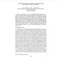
0.1 0.2 0.3 0.4 0.5 0.6 0.7 0.8 0.9 110.95Total system throughput vs. network load87QoS (minimum assigned relative rate) vs. network loadMTSMCSMPSMIGSIWFQCSDPSSystem throughput0.90.850.80.75MTSMCSMPSMIGSIWFQCSDPSMinimum assigned relative rate654320.710.65Total network loadFig. 2. Throughput vs. network load{ ∞[max E ∑ N]}∑{g} β s {α n g n (s)Y n (s) − f n [C n+1 (s)]} .{Y }s=0 n=1Now, we define G(C(t),Y(t),g(t)) D(t). LetS t ,thestate of the system at time t be defined as the augmentedvector X(t) =(C(t),g(t)). Note that the scheduler knowsthe channel capacities at the decision time, and therefore,the channel capacities are part of the state vector. However,before time t, the vector g(t)) is a random vector. At timet =0the system state is X(0). Then we have[ ∞]J ∗ (X(0)) max E ∑{g} β t G(C(t),Y(t),g(t))|X(0) .{Y }t=0(13)We would like to obtain the optimal policy Y ∗ (t) =µ ( ∗ C(t),g(t) ) at each time slot t that maximizes (13). Wecan rewrite the optimal income in the form of Bellman’srecursive equation for discounted infinite horizon problem atany time slot t [11], as follows:J ∗ (X(t)) = max {G(C(t),Y(t),g(t))Y (t)[+ βE g(t+1) J ∗ (C(t +1),g(t + 1)) ] }.If we denote the probability of g(t+1) = g k by ˆp g k, whereg k is the k th level quantized value for the channel capacity,we obtain:J ∗ (X(t)) = maxY (t) {G(C(t),Y(t),g(t))+ β ∑ kˆp g kJ ∗ ( C(t +1),g k) }. (14)Starting from X(t), the scheduler selects the user thatmaximizes the righthand side of (14), in which the firstterms represents the current income (as seen in the greedyalgorithm, MIGS) and the second term represents the incometo-go.It can be shown that this maximization is equivalent toselecting the user n in the following maximization problem:max {α ng n (t)+f n [C n (t)+r n ] − f n [C n (t)+r n − g n (t)]n⎡ ⎤0+ β ∑ .ˆp g kJ ∗ (C(t)+r −⎢ g n (t)⎥k⎣ . ⎦ ,gk )}.0Fig. 3.Fig. 4.00.1 0.2 0.3 0.4 0.5 0.6 0.7 0.8 0.9 1Total network loadMinimum assigned relative rate vs. network loadTotal system incomeSystem income vs. network load10510−1−2MTSMCS−3MPSMIGSIWFQCSDPS−4−50.1 0.2 0.3 0.4 0.5 0.6 0.7 0.8 0.9 12 x Total network loadTotal income vs. network loadIV. SIMULATIONS RESULTSIn order to evaluate the performance of our algorithms, wehave simulated a single-cell wireless system where users arerandomly distributed. We assume that path loss and shadowfading are compensated by a power allocation mechanismand the channel follows a Rayleigh fading distribution. Byconsidering the same noise level at all receivers, the receivedsignal power also follows a Rayleigh distribution. Here wehave assume that number of quantized levels of channelcapacities is Q =4. These levels and their probabilities are{1.0, 0.6, 0.4, 0.2} and {0.43, 0.24, 0.19, 0.14}, respectively.If R n is the assigned rate to user n, and r n is the reservedrate by that user, we define the minimum assigned relativerate over all users as η = min n { Rnr n}. This value can beconsidered as a measure of QoS; to support QoS for all users,we want η ≥ 1.First we present the simulation results for MIGS andcompare its performance with MTS, MCS, MPS, IWFQ, andCSDPS for a system with four users. The reserved rates ofthe four users are ρ[0.1, 0.2, 0.3, 0.4], where 0 ≤ ρ ≤ 1 isthe network load. Also, we assume that α n = 1000 for allusers.Throughput, minimum assigned relative rate, and totalincome are plotted in Figures 2-4, respectively. The penaltyfunction in the simulations is selected as in (5) with γ n =1.The horizontal axis in all these figures shows the networkload. As illustrated in Figure 2, MTS and MIGS achieve themaximum throughput (the expectation of maximum link capacity,E{max(g) =0.96}). MCS achieves a flat throughputwhich is equal to the average link capacity (E(g) =0.68).At low network loads, MPS tries to satisfy each user withIEEE Communications Society10310-7803-8533-0/04/$20.00 (c) 2004 IEEE