Solar Engineering a Condensed Course

2Lars BromanSolar Engineering - A Condensed Course°JyväskyläSolar Thermal Engineering according to Duffie and Beckman,and Solar Photovoltaic Engineering according to Martin GreenEdition November 2011© Lars Broman, lars.broman@stromstadakademi.se

3ForewordIn 1990, I had invited John Duffie from Solar Laboratory, University of Wisconsin, as GuestProfessor at Solar Energy Research Center, Dalarna University, to give a course in thermalsolar energy engineering. The course became the final test of a third edition of his andWilliam Beckman standard book to be published in the fall of 1990. Based on their book andmy lecture notes, I gave a course several times to engineering students during the comingyears and developed it into a 5-week full-time course at MSc and PhD level, first given as asummer course at Tingvall in 1998. Next summer, a similar summer course in photovoltaicsbased on the books on photovoltaics by Martin Green was given and in the fall the EuropeanSolar Engineering School started its 1-year master level program, where one of the courseswas thermal solar energy engineering, and another one PV solar energy engineering; bothbased on the previous experiences.Then, in 2000, I was asked to give a shorter course, equivalent to 2 weeks full-time study, insolar energy engineering at the Royal Institute of Technology KTH, Stockholm. I built thiscourse on the thermal and PV ESES courses, concentrating on the most important parts butstill giving a sound theoretical background. Over the years, I gave this course three moretimes at KTH and once at a University of Jyväskylä in Finland, gradually developing it into itspresent form. The present publication has until now been unpublished, used only as a coursecompendium. I hope that others now may find the text useful.Lars Broman, Falun 21 November 2011ContentsChapter 1 Solar Radiation 51.1 The Sun 51.2 Definitions 61.3 Direction of Beam Radiation 71.4 Ratio of Beam Radiation on Tilted Surface to that on Horizontal Surface, R b 91.5 ET Radiation on Horizontal Surface, G 0 101.6 Atmospheric Attenuation of Solar Radiation 111.7 Estimation of Clear Sky Radiation 121.8 Beam and Diffuse Components of Monthly Radiation 131.9 Radiation on Sloped Surfaces - Isotropic Sky 14Chapter 2 Selected Heat Transfer Topics 152.1 Electromagnetic Radiation 152.2 Radiation Intensity and Flux 172.3 IR Radiation Exchange Between Gray Surfaces 182.4 Sky Radiation 192.5 Radiation Heat Transfer Coefficient 202.6 Natural Convection Between Flat Parallel Plates 212.7 Wind Convection Coefficients 22Chapter 3 Radiation Characteristics for Opaque Materials 233.1 Absorptance, Emittance and Reflectance 233.2 Selective Surfaces 25Chapter 4 Radiation Transmission Through Glazing; Absorbed Radiation 264.1 Reflection of Radiation 26

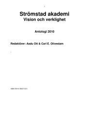
44.2 Optical Properties of Cover Systems 284.3 Absorbed Solar Radiation 294.4 Monthly Average Absorbed Radiation 30Chapter 5 Flat-Plate Collectors 315.1 Basic Flat-Plate Energy Balance Equation 315.2 Temperature Distributions in Flat-Plate Collectors 335.3 Collector Overall Heat Loss Coefficient 345.4 Collector Heat Removal Factor F R 355.5 Collector Characterization 365.6 Collector Tests 375.7 Energy Storage: Water Tanks 39Chapter 6 Semi Conductors and P-N Junctions 406.1 Semiconductors 416.2 P-N Junctions 42Chapter 7 The Behavior of Solar Cells 447.1 Absorption of light 447.2 Effect of light 467.3 One-diode model of PV cell 497.4 Cell propertiesChapter 8 Stand-Alone Photovoltaic Systems 528.1 Design and modules 528.2 Batteries 538.3 Household power systems 54Chapter 9 Grid Connected Photovoltaic Systems 559.1 Photovoltaic systems in buildings 559.2 Photovoltaic power plants 56Appendices 57A-1 Blackbody SpectrumA-2 Latitudes φ of Swedish Cities with Solar StationsA-3 Average Monthly Insolation Data for Swedish Cities and for JyväskyläA-4 Monthly Average Days, Dates, and DeclinationA-5 Spectral Distribution of Terrestrial Beam Radiation at AM2A-6 Properties of Air at One Atmosphere and Properties of MaterialsA-7 Algorithms for calculating monthly insolation on an arbitrarily tilted surfaceA-8 Answers to Selected Exercises(DB) refers to the corresponding sections in Duffie, J. A. and Beckman, W. A., SolarEngineering of Thermal Processes, John Wiley & Sons (3rd Ed. 2006).(AP) refers to the corresponding sections in Wenham, S. R., Green, M. A., and Watt, M. E.,Applied Photovoltaics, University of New South Wales, Sydney, Australia (1995). Someinformation is also included from Green, M. A., Solar Cells (1992).All illustrations by L Broman unless otherwise noted. Front page illustration indicates averageyearly insolation in kWh/m 2 on a surface that is tilted 30º towards south.

5Chapter 1Solar RadiationDB Ch 1-21.1 The SunDB 1.1-4Sun's diameter = 1.4×10 9 m (approx. 100× earth's dia.)Average distance = 1.5×10 11 m (approx. 100× sun's dia.The sun converts mass into energy (according to Einstein's equationnuclear fusion:2E = mc ) by means of4 p + 4e→K → α + 2e+ energy(1.1.1)The energy radiates from the sun's surface (the photosphere at approx. 6000 K) mainly aselectromagnetic radiation. The sun's power = 3.8×10 26 W, out of which the earth is irradiatedwith 1.7×10 17 W.The solar constant GSCequals the average power of the sun's radiation that reaches a unitarea, perpendicular to the rays, outside the atmosphere (thus extraterrestrial or ET), at earth'saverage distance from the sun:G =1367 [W/m 2 ] ( ± 1% measured uncertainty) (1.1.2)SCNote: The letter G is for irradiance = the radiative power per unit area and index sc is forsolar constant.The ET solar spectrum is close to the spectrum of a blackbody at 5777 K.Exercise 1.1.1Calculate the fraction and the power of the ET solar radiation that is ultraviolet (λ < 0.38 µm),visible (0.38 mm < λ < 0.78 µm), and infrared (λ > 0.78 µm) using the blackbody spectrumtables in Appendix 1.The sun-earth distance varies ± 1.65 % (2.5×10 9 m) - shortest around 1 January - giving ayearly variation of G 0:n360nG0n= 1367(1 + 0.033cos ) [W/m 2 ] (1.1.3)365where n is the day number, index 0 (zero) is for ET (no atmosphere), and index n is fornormal (⊥ to the rays).

61.2 DefinitionsDB 1.5, 2.1Air mass AM or m; m ≈ 1/cos θ z where θ z = the sun's zenith angle.Beam Radiation = radiation directly from the sun (creates shadows); index b. Radiation on aplane normal to the beam has also index n.Diffuse Radiation = radiation from the sun who's direction has been changed; also called skyradiation; index d.Total Solar Radiation = beam + diffuse radiation on a surface; no index. If on a tiltedsurface, index T.Global Radiation = total solar radiation on a horizontal surface; no index.Irradiance or intensity of solar radiation G [W/m 2 ].Insolation I [J/m 2 ,hour], H [J/m 2 ,day], H [J/m 2 ,day; monthly average].Swedish weather data: H [Wh/m 2 ,day], M [Wh/m 2 ,month].Solar time = standard time corrected for local longitude (+4 min. per degree east and -4 min.per degree west of standard meridian for the local time zone) and time equation E (variesbetween +15 min. in October and -15 min. in February due to earth's axis tilt and ellipticorbit). During the summer, one more hour has to be subtracted from the daylight saving time.In the following, all times are assumed to be solar time.Solar radiation = short wave radiation, 0.3µm < λ < 3µmLong wave radiation, λ > 3µmPyrheliometer measures beam (direct) radiation {bn} at normal incidence.Pyranometer measures global {b + d} or total {bT + dT}radiation.Exercise 1.2.1.M for Borlänge in July is 159 kWh/m 2 (average over many years). What is H for that placeand month?

71.3 Direction of Beam RadiationDB 1.6φ = latitude. Latitudes for Swedish solar measurement stations are given in Appendix 2.δ = the sun's declination (above or below the celestial equator):284 + nδ = 23.45sin(360 )(1.3.1)365β = the collector's tilt measured towards the horizontal plane.γ = the solar collector's azimuth angle = deviation from south, positive towards west, negativetowards east.γ s = the sun's azimuth angle.ω = the sun's hour angle measured in degrees (15°/h) from the meridian; positive in theafternoon, negative in the morning.θ = angle of incidence = angle between the solar collector normal and the (beam) radiation.θ z = (the sun's) zenith angle = 90° - α s (solar altitude angle).n = the day in the year (day number); for monthly average days, dates and declinations, seeAppendix 4.θ is a function of five variables:cosθ= sin δ sinφcos β − sin δ cosφsin β cosγ+ cos δ cosφcos β cosω+ cosδsinφsin β cosγcosω(1.3.2)+ cosδsin β sin γ sinωExercise 1.3.1Calculate the angle of incidence of beam radiation on a surface located in Stockholm on9 November at 1300 (solar time). Surface tilt is 30° towards south-southwest (i. e. 22.5° westof south).For a collector that is tilted towards south, γ = 0°, and Equation 1.3.2 is simplified intocosθ= sin δ sinφcos β − sin δ cosφsin β(1.3.3)+ cos δ cosφcos β cosω+ cosδsinφsin β cosωFor a horizontal surface, θ = θ z and β = 0°, which inserted into Equation 1.3.3 givescos θz= sin δ sinφ+ cosδcosφcosω(1.3.4)

8normalbeam radiationθβhorizontalnormalθβbeam radiation(φ - β)φEquatorFigure 1.3.1.South tilted surface with tilt β at latitude φ has the same incident angle θ as a horizontalsurface at latitude (φ - β):cosθ= cos( φ − β ) cosδcosω+ sin( φ − β ) sinδ(1.3.5)At 12 noon solar time, ω = 0, andθnoon= φ − β − δ(1.3.6)The hour angle at sunset ω s is given by Equation 1.3.4 for θ z = 90°:sinδsinφcosωs= − = − tanδtanφ(1.3.7)cosδcosφand, similarly, the hour angle ω s * for "sunset" for a south tilted surface is given by Equation1.3.5 for θ = 90°:∗cosωs= − tanδtan( φ − β )(1.3.8)unless the sun doesn't set for real before then!Exercise 1.3.2(a) at what times (solar time) does the sun set in Stockholm on 20 July and 9 November?(b) At what times (solar time) does the sun stop to shine (with beam radiation) onto a surfacein Stockholm that is tilted 60° towards south?From Equation 1.3.7, it is seen that the length of the day N is given by2N = arccos( − tanδtanφ)[hours] (1.3.9)15Exercise 1.3.3Calculate the length of the day in Stockholm on 9 November.

91.4 Ratio of Beam Radiation on Tilted Surface to that on HorizontalSurface, R bDB 1.8θG bTG bnθ zG bG bnβFigure 1.4.1. Beam radiation on horizontal and tilted surfaces.From Figure 1.4.1, it is seen that the ratio R b is given byRbGbT bn= = =(1.4.1)GbGGbncosθcosθzcosθcosθzFor insertion in Equation 1.4.1, cos θ and cos θ z are calculated using equations 1.3.2 and1.3.4, respectively.Exercise 1.4.1What is the ratio of beam radiation to that on a horizontal surface for the surface, time, anddate given in Exercise 1.3.1?For a south tilted surface, cos θ is given in the simplest way by Equation 1.3.5, givingcos( φ − β ) cosδcosω+ sin( φ − β )sinδRb=(1.4.2)cosφcosδcosω+ sinφsinδ

101.5 ET Radiation on Horizontal Surface, G 0DB 1.10As will be seen below, the extra-terrestrial solar radiation on a horizontal surface is a usefulquantity (see Section 1.8). The power of the radiation is given byG = 0cosθ(1.5.1)G0nzwhere G 0n is given by Equation 1.1.3 and cos θ z by Equation 1.3.4.Integration of Equation 1.5.1 from -ω s to + ω s (see Equation 1.3.7) gives the daily energy H0:24×3600G0πωsH0= n(cosφcosδsinωs+ sinφsinδ) (1.5.2)π180H0is approximately equal to H0for the month's average day (see Appendix 4) and M0equalsH0multiplied by the number of days in the month (and converted from MJ/day to kWh/mo.)Exercise 1.5.1What is H 0 for Stockholm on 14 November?Exercise 1.5.2What is M 0 for Stockholm and the month of November?

111.6 Atmospheric Attenuation of Solar RadiationDB 2.6Sweden has 13 meteorological stations with insolation data; see Appendix 2 and 3.Figure 1.6.1 shows how the sun's radiation is attenuated through Raley scattering andabsorption in O 3 , H 2 O and CO 2 :Figure 1.6.1 (from Duffie-Beckman)This figure is for AM 1. Attenuation is larger for AM 1.5 and AM 2. Since the Raleighscattering is higher for lower wavelengths, the diffuse sky radiation has an intensity maximumat 0.4 µm, making the clear sky blue. The spectral distribution of terrestrial beam radiation atAM 2 (and 23 km visibility) is given in the Table in Appendix 5.

121.7 Estimation of Clear Sky Radiation(Meinel and Meinel, replaces DB 2.8)The intensity of beam radiation varies with weather, air quality, altitude over sea level, andthe sun's zenith angle θ z . It is therefore impossible to tell the intensity without measuring it.There exists however a formula that gives an approximate estimate at moderate elevations,clear weather and dry air:Gbns≈ G exp[ −c(1/ cosθ) ](1.7.1)0nzwhere the empirical constants c = 0.347 and s = 0.678. The intensity of the diffuse skyradiation is about 10 % of the beam radiation for these circumstances, but may be muchhigher. (The total intensity is seldom over 1 .1G .)Exercise 1.7.1EstimateG when the sun is 25° over the horizon a clear day. Date 16 August.bnbn

131.8 Beam and Diffuse Components of Monthly RadiationDB 2.12Appendix 3 gives not only monthly global insolation but also the beam and diffusecomponents for the Swedish solar measurement sites. Normally, however, only globalinsolation is known. In order to estimate the components one can compare the measuredglobal insolation M with with the ET insolation M 0 , given by Equation 1.5.2 (times thenumber of days in the month). The ratio between M and M 0 is called monthly clearness indexK TM :K TM = M/M 0 (1.8.1)Qualitatively, it is obvious that the diffuse fraction M d /M decreases when K TM increases.Quantitatively, the following equations approximate the relation:For ω ≤ 81. 4°and 0.3≤ K ≤ 0. 8sTMMMd= (1.8.2 a)231.391−3.560KTM+ 4.189KTM− 2.137KTMFor ω ≥ 81. 4°and 0.3≤ K ≤ 0. 8sTMMMd231.311−3.022KTM+ 3.427KTM−1.821KTM= (1.8.2 b)[Ref. Erbs, D. G., Klein, S. A., and Duffie, J. A., Solar Energy 28(1982)293]Exercise 1.8.1Using the Erbs et al. formula, estimate the diffuse and beam fractions of global radiation inStockholm for November. How well does the formula estimate the measured fractions?

141.9 Radiation on Sloped Surfaces - Isotropic SkyDB 2.15,19,21The sky is brighter near the horizon and around the sun; isotropic sky is however anacceptable approximation. Under this assumption, I T for a tilted surface is given by1+cos β 1−cos βIT= IbRb+ Id( ) + Iρg( )(1.9.1)22where Rb= cosθ / cosθzis given by Equation 1.4.2 (for a south tilted surface) and ρ g = theground albedo (reflectance).Define R = I T /I. This givesIbId 1+cos β 1−cos βR = Rb+ ( ) + ρg( )(1.9.2)I I 22For monthly insolation on a tilted surface, we similarly getMTMbMd 1+cos β 1−cos βRM= = RMb+ ( ) + ρg( )(1.9.3)M M M 22where M d /M is a function of K TM , Equation 1.8.2 (or calculated from values given inAppendix 3).For a south tilted surface,RMb2=2∫∫ω0ω0s 'scosθdωcosθdωz(1.9.4)where cos θ z is given by Equation 1.3.4 and, for a south tilted surface, cos θ by Equation1.3.5; ω s ' = the sun's hour angle for "sunset" for a tilted surface (i. e. smallest angle of ω s andω s *), giving the following equations:whereR Mbcos( φ − β )cosδsinωs'+ ( π /180) ωs'sin(φ − β )sinδ= (1.9.5 a)cosφcosδsinω+ ( π /180) ω sinφsinδs∗ωs ' = min[ ωs= arccos( − tanφtanδ); ωs= arccos( − tan( φ − β ) tanδ] (1.9.5 b)Exercise 1.9.1Estimate the average monthly average radiation incident on a Stockholm collector that is tilted60° towards south, for the months June and November. Ground reflectance ρ = 0. 50 .Note: For a surface that is tilted to an arbitrary direction, the calculations are a bit morecomplicated, and usually a simulation program (like TRNSYS) is utilized. However, for asurface at mid-northern latitude and tilted 30-60° degrees between SE and SW, the insolationis not less than 95 % of that onto a south tilted surface (for some months and some tilts it caneven be higher). See also Appendix 7!sg

15Chapter 2Selected Heat Transfer TopicsDB Ch 3Radiation is approximately as important as conduction and convection in solar collectorswhere the energy flow per m 2 is about two orders of magnitude lower than for "conventional"processes (flat plate collector max. 1 kW/m 2 , electric oven hob typically 1 kW/dm 2 ).2.1 Electromagnetic RadiationThe electromagnetic spectrumDB 3.1-6Emission of thermal radiation is due to electrons, atoms and molecules changing energy statein a heated material; the emission is typically over a broad energy interval. The radiation ischaracterized by wavelength λ [m], frequency ν [Hz], and speed c 1 =c/n [m/s] where c = thespeed of light in vacuum and n = the refractive index of the material:λ ⋅ν = c c / n(2.1.1)1=Figure 2.1.1 Three electromagnetic spectra. Visible light is the interval 0.38 < λ < 0.78 µm,ultra violet light λ < 0.38 µm, and infrared radiation λ > 0.78 µm (from Duffie-Beckman).PhotonsLight consists of photons, whose energy E is related to the frequency ν:E = h⋅ν (2.1.2)where Planck's constant h = 6.6256⋅10 -34 [Js]

16Blackbody radiationAn ideal blackbody absorbs and emits the maximum amount of radiation: Cavity 100 %,"pitch black" 99 %, "black" paint 90-95 %.Planck's radiation lawThermal radiation has wavelengths between 0.2 µm (200 nm) and 1000 µm (1 mm). Thespectrum of blackbody radiation is, according to Planck:dEC1= Eλ b=(2.1.3)5∂A∂λλ [ exp( C2/ λT) −1]where C 1 = 3.74⋅10 -16 [m 2 W] and C 2 = 0.0144 [m⋅K].Wien's displacement lawDerivation of Planck's radiation law gives Wien's displacement law:λ max ⋅T = 2898 [µm⋅K]. (2.1.4)Stefan-Boltzmann's radiation lawIntegration of Planck's radiation law gives Stefan-Boltzmann's radiation law:dEdAσ4= Eb= T(2.1.5)where Stefan-Boltzmann's constant σ = 5.67⋅10 -8 [W/m 2 ,K 4 ].Radiation tablesThe blackbody spectrum is tabled in Appendix 1.Table 1 gives the fraction of blackbody radiant energy ∆f between previous λT and presentλT [µm K] for different λT-values.Table 2 gives the fraction of blackbody radiant energy ∆f between zero and λT [µm K] foreven fractional increments.Exercise 2.1.1Assume the sun is a blackbody at 5777 K. (a) What is the wavelength at which the maximummonochromatic emissive power occurs? (b) At what wavelength λ m is half of the emittedradiation below λ m and half above λ m (λ m = "median wavelength").

172.2 Radiation Intensity and FluxDB 3.7In this Section, intensity and flux are defined in a general sense, i. e. for radiation emitted,absorbed or just passing a real or imaginary plane.Intensity I:Flux q:dEI = ⊥ mot A [W/m 2 ,sterradian] (2.2.1)∂ A ∂ω2ππ / 2∫ φ = 0 ∫θ=q = I cosθsinθdθdφ[W/m 2 ] (2.2.2)0Here, θ is the exit (or incident) angle (measured from the normal) and φ is the "azimuth"angle. For the special case a surface where I = constant independently of θ and φ, integrationgives:q = π ⋅ I(2.2.3)Such a surface (where I = constant) is called diffuse or Lambertian. An ideal blackbody isdiffuse:Ib= E b/π(2.2.4)This applies also to monochromatic radiation, so for a particular λ we get:I = E π(2.2.5)λ b λb/Equation 2.2.4 complements 2.1.5 (Stefan-Boltzmann), and Equation 2.2.5 complements2.1.3 (Planck).Integrating (2.2.2) over all φ givesdq= π ⋅ I ⋅sin 2θ(for a Lambertian surface).dθI∆ωA∆AφθFigure 2.2.1

182.3 IR Radiation Exchange Between Gray SurfacesDB3.8We identify two special (idealized) cases.(1) Exchange of radiation between two large parallel surfaces:QAσ ( T1− T2)=1/ ε + 1/ ε −11424[W/m 2 ] (2.3.1)(2) Exchange of radiation between a small object (A 1 ) and a large enclosure:Q4 41 1 1 1T2= ε A σ ( T − ) [W] (2.3.2)

192.4 Sky RadiationDB 3.9A solar collector exchanges radiative energy with the surroundings according to Equation2.3.2:4 4Q = ε Aσ( T − )(2.4.1)T SHere, TS= Ta⋅Ccorr.(2.4.2)where Ccorr.varies with the humidity of the of the air (≈ 1 when humid or cloudy, ≈ 0.9 whenclear and dry air). Usually, Ccorr.= 1 is a good enough approximation.

202.5 Radiation Heat Transfer CoefficientDB 3.10We want Equation 2.3.1 written asQ = A hr ( T − 1)(2.5.1)1 2Twhich, from Equation (2.3.1), gives the heat transfer coefficient h r :2σ ( T2+ T1)( T2+ T1)h r=(2.5.2)1/ ε + 1/ ε −1122In Equation (2.5.2), the nominator can be approximated byT 2 and T 1 . (Verify this!)3σ where T is the average of4 TExercise 2.5.1The plate and cover of a flat-plate collector are large in extent, parallel, and 25 mm apart. Theemittance of the plate is 0.15 and its temperature is 70°C. The emittance of the glass cover is0.88 and its temperature 50°C. Calculate the radiation exchange between the surfaces Q/A andthe heat transfer coefficient h r .

212.6 Natural Convection Between Flat Parallel PlatesDB 3.11-12The dimensionless Raleigh number Ra is a function of the gas' (usually the air's) properties (atthe actual temperature) and the temperature difference between the plates ∆T:Ra =g ⋅ ∆T⋅ Lν ⋅α⋅T3(2.6.1)where g = gravitational constant (9.81 m/s 2 ), L = plate spacing, α = thermal diffusivity, andv = kinematic viscosity (= Pr⋅α where Pr is the dimensionless Prandtl number).For parallel plates, the dimensionless Nusselt number Nu = 1 for pure conduction, and whenboth conduction and convection takes place, given byh hLNu = =(2.6.2)k / L kwhere h = heat transfer coefficient and k = thermal conductivity.Some useful properties of air are found in Appendix 6.When convection takes place, Nu is given by Equation 2.6.3:1.6+⎤ ⎡⎛⎞ ⎤⎥⎢⎡ 1/ 3Nu ⎡ 1708(sin1.8β) ⎤ 1708 Racosβ= 1 + 1.44⎢1−1 − ⎥ + ⎢⎜⎟ − 1 ⎥⎣ Racosβ ⎦⎣Racosβ ⎦ ⎢⎣⎝ 5830 ⎠ ⎥(2.6.3)⎦where the meaning of the + exponent is that only positive values of the square brackets are tobe used (i. e., use zero if bracket is negative).Exercise 2.6.1Find the convection heat transfer coefficient h (including conduction!) between two parallelplates separated by 25 mm with 45° tilt. The lower plate is at 70°C and the upper plate at50°C.Note: The curve for 75° tilt of the solar collector is also good for vertical (tilt 90°).Convection in a solar collector can be suppressed by various means like honeycomb andaerogel. Most common is a flat film between the glazing and the absorber plate.Exercise 2.6.2What would h in Exercise 2.6.1 approximately become if a flat film is added between theglazing and the plate? Assume that the temperature of the film is 60°C.+

222.7 Wind Convection CoefficientsDB 3.15Recommendation:0.6⎡ 8.6V⎤h w= max⎢5,0. 4 ⎥ [W/m 2 C] (2.8.1)⎣ L ⎦where h w = the heat transfer coefficient for wind.for wind speed V [m/s] and a collector on a house withL = 3 volume .World average value V = 5 m/s ⇒ h ≈ 10 [W/m 2 C] (see also Exercise 2.7.1).wWhen only absorber and ambient temperatures are known, but not the glazing's temperatureTg(and this is of course normally the case!) the procedure is to guess Tg, then calculate theradiative and convective losses both absorber → glazing and glazing → ambient, and keepadjusting Tguntil the two match. For more information see Section 5.3 (and Duffie-Beckman,Chapter 6).Exercise 2.7.1(a) What L makes h w = 10 W/m 2 ,K for V = 5 m/s?(b) How much will h w change if L is doubled or halved?

23Chapter 3Radiation Characteristics for Opaque MaterialsDB Ch 43.1 Absorptance, Emittance and ReflectanceDB 4.1-6, 11, 13Absorptance and emittanceε λ / α λ( µ , φ)= emittance/absorptance at wavelength λ and direction θ, φ (µ = cos θ).ε / α ( µ , φ)= emittance/absorptance at all wavelengths and direction θ, φ.ε /αε λ / αλ= emittance/absorptance at all wavelengths, all directions.= emittance/absorptance at wavelength λ, all directions.Absorptance α λ( µ , φ)and emittance ε λ( µ , φ)are surface properties:Iλ,a(µ , φ)αλ( µ , φ)= (3.1.1)I ( µ , φ)λ,iIλ( µ , φ)ελ( µ , φ)= (3.1.2)IλbAbsorptance α and emittance ε can now be calculated by means of integrating the I:s. Theresulting complicated equations are much simplified if we (i) assume that α and ε areindependent of µ and φ (which is rather true) and (ii) that, in the case of α, we restrictourselves to the solar spectrum (indicated by subscript s):αε∫ ∞α Esdλ= 0 λ λE∫ ∞ε Ebdλ= 0 λ λEbs(3.1.3)(3.1.4)Note that α and ε are not only dependent on the properties of the surface but also of thespectrum; in the case of ε therefore on the temperature of the radiating surface.Kirchhoff's lawFor a body in thermal equilibrium with a surrounding (evacuated) enclosure, absorbed andemitted energy must be equal. From this fact can we conclude that, in this case, α and ε forthis body must be the same. Then this must be true for all λ:s. This is important, because,since αλand ελare surface properties only,must hold for all surfaces.ελ= α λ(3.1.5)

24ReflectanceReflectance ρ may be specular (as at an ideal mirror), diffuse, or a mixture of both. Themonochromatic reflectance ρλis a surface property, but the total reflectance ρ is alsodependent on the spectrum.Relationships between absorptance, emittance, and reflectanceAll incident light that is not absorbed is reflected. Therefore,ρ + α = 1 (3.1.6)Restricting ourselves to the monocromatic quantities, emittance can be included:ρ α = ρ + ε = 1(3.1.7)λ+λ λ λFinally, note that while ε is determined by the surface's properties and temperature, α (andthus ρ) depends on an external factor, the spectral distribution of the incident radiation.Calculation of emittance and absorptanceThis is done by integration, usually by means of numerical integration; i. e. summation over anumber of equal energy intervals of the spectrum:nn1 1ε = ε λ= 1−ρ λ j(3.1.8)∑∑jn j= 1 n j=1nn1 1α = α λ= 1−ρ λ j(3.1.9)∑∑jn j = 1 n j = 1Exercise 3.1.1Calculate the absorptance α for the terrestrial solar spectrum in Appendix 5 of a(hypothetical) surface with a non-constant ρ λ= 0. 05λ[λ in µm] by means of numericalintegration.Exercise 3.1.2Calculate the emittance ε for the same surface at temperature 400 K using Table 2 inAppendix 1.Angular dependence of solar absorptanceFor a typical surface, α decreases at large incidence angles. This will be taken into account inthe angular dependence of the transmittance-absorptance product (τα); see Section 5.6. Alsospecularly reflecting surfaces may show such decrease, especially degraded surfaces.

253.2 Selective SurfacesDB 4.8-10An absorber with large αλfor the region of the solar spectrum and a small ελfor the longwaveregion would be very effective. An absorber with such a surface is called selective.There are some different mechanisms employed in making selective surfaces:(a) Thin (a few µm) black surface (black chrome, black nickel, copper oxide, ...) on areflective surface.(b) Enhanced absorptance through successive (specular) reflection in V-troughs.(c) Thin black surface + micro structure (like the black nickel sputtered aluminum surface ofthe Swedish Sunstrip ® absorber).Exercise 3.2.1Calculate the absorptance for blackbody radiation from a source at 5777 K and the emittanceat surface temperatures 100 C and 500 C (using Appendix 1, Table 1) for a surface withρλ= 0.1 for λ < 3 µm, and ρλ= 0.9 for λ > 3 µm. (This is a hypothetical, but not terriblyunrealistic good selective surface.) Is the emittance dependent on the surface temperature?Note that a large α (for solar radiation) is even more important than a small ε for thermalradiation. The quantity α/ε is sometimes referred to as the selectivity of the absorber.

26Chapter 4Radiation Transmission Through Glazing; Absorbed RadiationDB Ch 54.1 Reflection of RadiationDB 5.1The reflectance r is given by Fresnel's expressions for reflection of unpolarized light passingfrom one medium with refractive index n 1 to another medium with refractive index n 2 :r ⊥ =r // =2sin ( θ2−θ1)2sin ( θ + θ )212tan ( θ2−θ1)2tan ( θ + θ )21(4.1.1)(4.1.2)wherer =IIri1=21sinθ1n2sin(r ⊥ + r // ) (4.1.3)n = θ (Snell's law) (4.1.4)2At normal incidence (θ = 0):n1= 1 (air) and n = nr( 1 20) = =I ⎜ ⎟ i ⎝ n1+ n2⎠2:2I ⎛ n − n ⎞r⎜(4.1.5)2Ir ⎛ n −1⎞r( 0) = = ⎜ ⎟ (4.1.6)I ⎝ n + 1 ⎠iExercise 4.1.1Calculate the reflectance of one surface of glass at normal incidence and at θ = 60°. Theaverage index of refraction of glass for the solar spectrum is 1.526.A slab or film of transparent material has two surfaces:1r(1-r) 2 r1-r(1-r)retc.(1-r) 2Figure 4.1.1. Transmission through one nonabsorbing cover.

27From Figure 4.1.1 we get the following expression for transmission τ :Similarly,τ ⊥ = (1 - r ⊥ ) 2 ∑ ∞ ( r 2n ⊥ ) = (1 - r ⊥ ) 2 /(1-r 2 ⊥ ) = (1-r ⊥ )/(1+r ⊥ ) (4.1.7)=0nτ // = (1 - r // )/(1 + r // ) (4.1.8)Note that r ⊥ ≠ r // except for θ = 0°. Finally, for unpolarized light,1τr= (τ⊥ + τ // ) (4.1.9)2Subscript r shows that this is the transmittance due to reflection.Exercise 4.1.2Calculate the transmittance of two covers of nonabsorbing glass at normal incidence and atθ = 60°.

284.2 Optical Properties of Cover SystemsDB 5.2-6Absorption by glazing is given bydI = −IKdx(4.2.1)where K = extinction coefficient; K is between 4 m -1 (for clear white glass) and 32 m -1 (forgreenish window glass). Integration from 0 to L / cosθ2(where L is the thickness of thecover) gives transmittance due to absorption,I⎛ ⎞=transmitted KLτ= exp⎜ −⎟a(4.2.2)Iincident ⎝ cosθ2 ⎠where θ 2 is given by Snell's law (providing θ 1 is known).With very good approximation, τ for a slab is given byτ = τ aτ r(4.2.3)Absorptance and reflectance of a slab is then given byandα = 1 −τ a(4.2.4)ρ1 −τ−α= τ −τ(4.2.5)=aExercise 4.2.1Calculate the transmittance, reflectance, and absorptance of a single glass cover, 3 mm thick,at an angle of 45°. The extinction coefficient of the glass is 32 m -1 .Transmittance of diffuse radiationDiffuse radiation hits the surface at all incident angles between 0° and 90°. An astonishinglygood approximation is to use the effective incident angle θe= 60°.Transmittance-absorptance product (τατα)Regard (τα) as one symbol for one property of the combination glazing + absorber. (τα) isslightly larger than τ⋅α. A good approximation is(τα) = 1.01⋅τ⋅α (4.2.6)Exercise 4.2.2For a collector with the cover in Exercise 4.2.1 and an absorber plate with α = 0.90(independent of direction), calculate (τα) for θ = 45°.The angular dependence of (τα) is given by the so-called incidence angle modifier; seeSection 5.6.

294.3 Absorbed Solar RadiationDB 5.9Hourly values of the intensity ITon a tilted surface are given by Equation 1.9.1 withRb= IbT/ Iband isotropic diffuse light. Multiplication with appropriate (τα)-values yieldsabsorbed radiation S:⎛ 1+cos β ⎞⎛1−cos β ⎞S = IbRb( τα )b+ Id⎜ ⎟(τα )d+ ρg( Ib+ Id) ⎜ ⎟(τα )g(4.3.1)⎝ 2 ⎠⎝ 2 ⎠Note that Iband Idare for a horizontal surface. In order to calculate(is also needed to calculate Rb). For (τα )dand (τα )g, use θe= 60°.(τα )b, θ must be knownExercise 4.3.1For the hour between 11 and 12 on a clear winter day in southern Europe, I = 1.79 MJ/m 2 ,Ib= 1.38 MJ/m 2 , and Id= 0.41 MJ/m 2 . Ground reflectance is 0.6. For this hour, θ for thebeam radiation is 17° and Rb= 2.11. A collector with one glass cover is sloped 60° to thesouth. The glass has KL = 0.0370 and the absorptance of the plate is 0.93 (at all angles). Usingthe isotropic diffuse model (Equation 4.3.1), calculate the absorbed radiation per unit area ofthe absorber.Equation 4.3.1 is terribly similar to expression 1.9.1 for IT. It is therefore natural to introducea new quantity, (τα )av, defined byS = (τα ) I (4.3.2)av Tor, for instantaneous values,S = (τα ) G (4.3.3)av T

304.4 Monthly Average Absorbed RadiationDB 5.10The expression for SMlooks like this:⎛ 1+cos β ⎞⎛1−cos β ⎞SM= MbRMb( τα)b+ Md( τα )d ⎜ ⎟ + Mρg( τα )g ⎜ ⎟ (4.4.1)⎝ 2 ⎠⎝ 2 ⎠Calculation of SM(for south-tilted surface):(1) M is measured (or given, e. g. in Appendix 3).(2) M0is calculated using Equation 1.5.2 (and following).(3) Calculate clearness index K TM= M / M0.(4) Finding Md/ M = f ( KTM) as outlined in Section 1.8. If Mdis known (e. g. fromAppendix 3), points (2) - (4) can be omitted.(5) Mb= M − Md(6) Average incident angle for beam radiation equals approximately θ at 2.5 hours before orafter noon on the average day; θ is calculated with Equation 1.3.3.(7) θefor diffuse and sky components approximately equals 60°.(8) τ is calculated for θ and θeusing the methods in 4.1 and 4.2.(9) knowing α, (τα) is calculated for the two angles using Equation 4.2.6.(10) RMbis calculated using Equations 1.9.5 a and b.(11) Now SMcan be calculated with Equation 4.4.1.Exercise 4.4.1Calculate SMfor a 45° south-tilted collector in Stockholm in August. The collector has oneglass with KL = 0.0125 and α for the absorber is 0.90. Ground reflectance ρ = 0. 50 .g

31Chapter 5Flat-Plate CollectorsDB Ch 6, 8, 105.1 Basic Flat-Plate Energy Balance EquationDB 6.1-2A solar collector is (in principle) a heat exchanger radiation → (e. g.) hot water. A solarcollector is characterized by low and variable energy flow, and that radiation is an importantpart of the heat balance.Figure 5.1.1. Typical solar collector. Gummipackning = rubber gasket. Glas = glass.Plastfilm = plastic film. Absorbatorband ... = absorber strips of aluminum withwater channels and selective coating on the top side. Diffusionsspärr ... == diffusion barrier made of aluminum foil. Mineralull = mineral wool.Solfångarlåda ... = Collector box of galvanized steel tin.The useful energyQufrom a solar collector is given byQu= A S −U( T − T )](5.1.1)c[ L pm awhere Ac= collector area, S = absorbed energy per m 2 absorber area, UL= heat losscoefficient, Tpm= the absorber surface's average temperature, and Ta= ambient temperature(subscripts p for plate and m for mean value).

32Problem: It is difficult both to measure and to calculate Tpmtherefore instead use the following expression:. Instead of Equation 5.1.1 weQu= A F S −U( T − T )](5.1.2)cR[ L i awhere FR= the collector's heat removal factor and Ti= the inlet water temperature. Insertionof S from Equation 4.3.3 changes this equation intoQu= A F ( τα ) I − F U ( T − T )](5.1.3)c[ R T R L i aThis is Duffie-Beckman's most important formula. (τα ) is short forEquation 4.3.2/4.3.3.(τα )avas defined byNormally hourly values are used: S [J/m 2 ,h]; then S is calculated from IT. Remember that1 kWh = 3.6 MJ.Especially in tests, instantaneous values are used: S [W/m 2 ]; then S is calculated fromThe efficiency η of a solar collector is given by∫c∫Qudtη =(5.1.4)A G dtTGT.

335.2 Temperature Distributions in Flat-Plate CollectorsDB 6.3The temperature Tpof an absorber plate is not constant over the surface, but varies both inparallel with and perpendicular to the water (or fluid) channels.Under operation, the outlet temperature is higher than the inlet temperature, so absorbertemperature increases in parallel with the water flow. Heat is conducted through the absorbertowards the water channels, so the absorber temperature perpendicular to the channels islowest at the channels and highest in the middle between them.Finally, there is a temperature difference between the channel (tube) and the water. Theabsorber temperature is therefore on the average higher than the water inlet temperature;hence the factor FRin Equation 5.1.2.

345.3 Collector Overall Heat Loss CoefficientDB 6.4The heat loss coefficient UL[W/m 2 K] is the sum of the top, bottom, and edge losscoefficients:U = U + U + U(5.3.1)LtbeThe top loss coefficient is due to convection and radiation, and the two others to heatconduction. For an efficient collector, all three are kept low (as low as it is economical).Bottom and edge losses are minimized by means of adequate insulation.The top loss coefficient is more difficult to make low without decreasing S. An extra glass orplastic film between the glass and the absorber decreases convection losses, but also S getslower. A selective absorber surface gives much lower radiation losses than an absorbercovered with black paint.(One more way to minimize losses is to keep the average temperature of the absorber as lowas possible, since the heat losses from an absorber are proportional to the difference betweenthis temperature and the ambient temperature.)ULcan be calculated from the optical, geometrical and thermal properties of the collector,and is typically between 2 and 8 W/m 2 K. UL(or, rather, F RUL) can also be measured, andthis is always done by collector manufacturers. In the present treatment it will be assumed thatmeasured heat loss factors are available. The interested reader, who wants to learn theintricacies of calculating a collector's U , is referred to Duffie-Beckman.L

355.4 Collector Heat Removal Factor F RDB 6.5-7The heat removal factor FRis the product of two factors, the collector efficiency factor F′and the collector flow factor F ′′ . F′ compensates for the fact that the temperature of anabsorber cross section perpendicular to the water flow is higher than the temperature of thewater. F′ ≈ F (Section 5.6).avF ′′ compensates for the fact that the average temperature along the water flow Tavis higherthan the inlet temperature Ti.

365.5 Collector CharacterizationDB 6.15-16Measured collector performance and performance calculated according to the principlesmentioned above agree very well. The collector is also well described by the (stationary)Equation 5.1.3, possibly complemented by the collector's dynamic performance.This equation contains three parameters, ULand FRwhich are constant or varies withtemperature, and (τα ) that is constant or varies with incidence angle θi.The collector's instantaneous efficiency ηiis given byQ F U ( T − T )uR L i aηi= = FR( τα ) −(5.5.1)AcGTGTIn the next section, the incidence angle modifierK= τα ) /( τα ) f ( θ )(5.5.2)τα(n=bwhere the parameter bois part of the expression, will be explained. This leaves us with threebasic solar collector parameters:F (τα ) indicating how energy is absorbed;RnF RULindicating how energy is lost; andboindicating the dependence of the incidence angle θ b.

375.6 Collector TestsDB 6.17-20A (complete) solar collector test consists of three measurements: instantaneous efficiency at near normal incidence; dependence on the incidence angle; and the collector's time constant.In order to determine ηi, mass flow m& , outlet temperature To, and inlet temperature Ti, solarradiation intensity GT, and wind speed V are measured, givingm C ( T − T )= &p o iηi(5.6.1)AcGTThe so obtained ηiis inserted into Equation 5.5.1.η i1η 0 = F R ( τα)slope = F R U L00∆TGTTi− Ta=GTFigure 5.6.1Exercise 5.6.1A water heating collector with an aperture area of 4.10 m 2 is tested with the beam radiationnearly normal to the plane of the collector, giving the following information:Qu[MJ/hr] GT[W/m 2 ] Ti[°C] Ta[°C]9.05 864 18.2 10.01.98 894 84.1 10.0What are the FR(τα )nand F RULfor this collector, based upon aperture area? (In practice,tests produce multiple data points and a least squares fit would be used to find the bestconstants.)

38In Europe, another expression is normally used, namelyQ F U ( T − T )uav L av aηi= = Fav( τα ) −(5.6.2)AcGTGTwhere Tav= ( To+ Ti) / 2 and the relation between FRand Favis given byFR⎛⎜A = 1 +cFavUFav⎝ 2mC&pL⎞⎟⎠−1(5.6.3)Inserting the incidence angle moderator5.1.3 changes this intowhereQuKτα(as defined by Equation 5.5.2) into Equation= A F G Kτα ( τα ) −U( T − T )](5.6.4)cR[ Tn L i a⎛ 1 ⎞K τα = 1+bo⎜ −1⎟(5.6.5)⎝ cosθ⎠and the incidence angle modifier coefficient botypically is between -0.10 and -0.20.

395.7 Energy Storage: Water TanksDB 8.3-4, 10.10Energy (heat) can be stored in many forms, commonly as heat without phase change (sensibleheat) in water.The useful one-cycle capacity of a water tank is given byQs= ( mC ) ∆T[J] (5.7.1)psswhere ∆Tsis the temperature range. For a fully mixed (non-stratified) tank, we get thefollowing power balancedTs( mCp)s= Qu− Ls− ( UA)s(Ts− Ta')(5.7.2)dtwhere the three terms represent the energy input from the collector, the load, and the loss,respectively. Numerical integration of Equation 5.7.2 is done by calculating a new+temperature ( T ) e. g. once per hour:sT+s= Ts∆t+( mC )ps[ Qu− Ls− ( UA)( Tss− Ta')](5.7.3)A modern solar heating system increasingly frequently includes a stratified water storagetank. Such a tank is arranged so cold water is taken from the tank's bottom to the solarcollector loop (via a heat exchanger), and hot water from the collector loop is added at the topor, even better, at the position in the tank where the temperature is the same as the water fromthe collector.Such a tank is usually a part of a so-called low-flow system: Cold water enters the solarcollector and passes it so slowly that it is quite hot when it gets back to the heat exchanger.Such a system delivers much useful heat, lowers the requirement of auxiliary heat, but is stilleffective, since the low inlet temperature brings the average absorber temperature (and thusthe heat losses) down.Solar fractionThe solar fraction, i. e. the percentage of the (seasonal or yearly) heat load is increasinglyused as a measure of how well a system performs. Recent research at SERC in Sweden has asan example shown that the solar fraction of a typical summer season hot water system can bedoubled if the classical high-flow system with a copper tubing coil in the bottom of thestorage tank is replaced with a low-flow system with efficient so called SST heat exchangerand a stratified tank, without increasing the collector area.

40Chapter 6Semi Conductors and P-N Junctions6.1 Semiconductors(AP 2.1-2)Valence bands have electrons stuck to the covalent bonds in the lattice. Conduction bandsmay have free electrons. Between the bands is a forbidden band with band gap E G . The Fermilevel E F is close to mid-gap in pure semiconductors. Semiconductors have E G = 0.4-4 eV.Insulators have E G >> 4 eV. Metals have no band gap.EE FMetal Semiconductor InsulatorFigure 6.1.1. Bands (bottom to top): Valence band, forbidden band, conduction band.Semiconductors are (normally) crystals with diamond lattice and each atom surrounded byfour atoms. They can be group IV atoms (Si, Ge) or a mixture of group III (Ga, Cu, In) andgroup V (As, Se, Sb) atoms.SiSiSiSiSiSi Si SiSi Si Si SiFigure 6.1.2. Two-dimensional analogy of a small part of a Si crystal witha thermally generated electron-hole pair.Neither a filled valence band nor an empty conduction band can conduct any current. Insemiconductors, Fermi-Dirac statistics however permits (at room temperature) a small amountof electrons in the conduction band, leaving holes behind in the valence band. Both carriersmay conduct current, thus making the crystal "semiconductive". (Analogy: Parking garage w.first floor totally filled and second floor empty + move one car from first to second floor.)

41By doping a semiconductor with Group III or V atoms, free carriers can be created. Theenergy needed to brake the bond of the extra carrier, approx. 0.02 eV, is so low that inprinciple a free carrier per doping atom is created.SiSiSiSiSiSi As SiSi Si Si SiFigure 6.1.3. Small part of Si crystal doped with donor atoms from Group V (As),resulting in free negative carriers (electrons) and bound positive charges.SiSiSiSiSiSi In SiSi Si Si SiFigure 6.1.4. Small part of Si crystal doped with acceptor atoms from Group III (In),resulting in free positive carriers (holes) and bound negative charges.More on semiconductors for solar cell applications is found in Section 7.4

426.2 P-N Junctions(AP 2.5)Doping a semiconductor with Group III atoms moves the Fermi level close to the valenceband; see Figure 6.2.1 (a). (b) Doping a semiconductor with Group V atoms moves the Fermilevel close to the conduction band; see Figure 6.2.1 (b).PNEE FnE Fp(a)(b)Figure 6.2.1. (a) Semiconductor doped with acceptor atoms.(b) Semiconductor doped with donor atoms.A p-n junction is formed by bringing the p-type and n-type regions together in a conceptualexperiment. The characteristics of the equilibrium situation can be found by consideringFermi levels: A system in thermal equilibrium can have only one Fermi level. See Figure6.2.2.PNEtransitionregionE G E 1 = kT ln(N V /N A ) E cE FE 2 = kT ln(N C /N D )E vFigure 6.2.2. p-n junction. N V = effective density of states in the valence band.N A = density of acceptors. N C = effective density of states in the conductionband. N D = density of donors. (For Si, N V = 1⋅10 25 m -3 and N C = 3⋅10 25 m -3 .)

43When joined, the excess holes in the p-type material flow by diffusion to the n-type, while theelectrons flow by diffusion from n-type to p-type as a result of the carrier concentrationgradients across the junction. They leave behind exposed charges on dopant atom sites, fixedin the crystal lattice. An electric field Ê therefore builds up in the so-called "depletionregion" around the junction to stop the flow.hePNVFigure 6.2.3. (a) Application of a voltage to a p-n junction. (b) Shape of electric field.If a voltage is applied to the junction as shown in Figure 6.2.3, Ê will be reduced and acurrent flows through the diode (if the external voltage is large enough). If a reverse voltage isapplied, no current will flow (or, rather, a low current I 0 due to thermally generated electronholepairs). This gives the diode law:I = I 0 [exp(qV/nkT) - 1] (6.2.1)where I 0 is called "dark saturation current", q = electric unit charge, k = Boltzmann's constant,T = absolute temperature, and n = the ideality factor, a number between 1 and 2 whichtypically increases when the current decreases. Note that kT /q = 0.026 V for T = 300 K.IT 2 T 10.6 VFigure 6.2.4. The diode law for silicon. T 2 > T 1 . The temperature shift is approx. 2 mV/°C.Exercise 6.2.1I 0 = 5.0⋅10 -12 A for a diode. Draw an I-V characteristics for this diode.What is V for I = 2.0 A? Assume T = 300 K and n = 1.

44Chapter 7The Behavior of Solar Cells7.1 Absorption of light(AP 2.3-5)Fundamental absorption = the annihilation of photons by the excitation of an electron fromthe valence band upp to the conduction band, leaving a hole behind. The energy differencebetween the initial and the final state is equal to the photon's energy:E f - E i = hν (7.1.1)For a free particle, kinetic energy and momentum are related byE k [= mv 2 /2 = (mv) 2 /2m] = p 2 /2m (7.1.2)Similarly for electrons in the conduction band E c and holes in the valence band E v :E - E c = p 2 /2m e * and E v - E = p 2 /2m h * (7.1.3 a, b)where p is known as the crystal momentum, and m e * and m h * are the "effective masses" of thecarriers in the lattice. From Equation (7.1.3) is seen both that the conduction band has itsminimum and the valence band its maximum for p = 0; this is called a direct-band-gap devicelike GaAs. Si and Ge are however examples of indirect-band-gap devices where theconduction band minimum occurs at a finite momentum p 0 . Then Equation (7.1.3 a) isreplaced byE - E c = (p - p 0 ) 2 /2m e * (7.1.4)The situations are presented in Figure 7.1.1:Energy Energy Phonon emissionPhonon absorptionE cE fE chνhυ=E g +E p hν =E g -E pE v E v p 0E i crystal crystalmomentummomentum(a)(b)Figure 7.1.1. Energy-crystal relationships near the band edges forelectrons in the conduction band and holes in the valence band of(a) a direct-band-gap device, (b) an indirect-band-gap device.For transitions, see text.

45In a direct-band-gap semiconductor, a photon is readily absorbed within a few µm if itsenergy hf > E g = E c -E v . In an indirect-band-gap semiconductor, a phonon (= a quantumcorresponding to coordinated vibration in the crystal structure) must be absorbed or emitted (aphonon has high momentum in comparison with photons). Therefore, if we want low-energyphotons of the near-infrared absorbed, a device thickness of 100 µm or more is required.These are the energy limits in crystalline Si for phonon-absorption process, phonon-emissionprocess, and direct process (at T = 0 K), respectively:E g1 (0) = 1.1557 eVE g2 (0) = 2.5 eVE gd (0) = 3.2 eVAt room temperature, E g for Si is approximated to 1.1 eV.A useful relation for photons: λ [µm] × hf [eV] = 1.24.When an absorbed photon has lower energy than E g , no electron is lifted from the valenceband to the conduction band, and all its energy is dissipated as thermal energy in the device.When a photon has higher energy than E g , the remaining energy of an absorbed photon isdissipated as thermal energy in the device, and thus lost. The fraction of the photon's energythat is available for the process is therefore:E useful /hν = 0 for hν < E g andE useful /hν = E g /hffor hfν> E g(7.1.5)The number of electrons lifted into the conduction band per incident photon is called thequantum efficiency Q E . Ideally, the internal Q E = 1 for hν > E g (and = 0 for hν < E g ). Theexternal Q E includes the transmittance τ of the surface of the device. For a non-treatedsurface, τ can be rather low. Surface reflectance ρ (= 1 - τ) for normal incidence is given bythe equation2 2( n −1)+ kρ =(7.1.6)2 2( n + 1) + kwhere the (complex) index of refraction of a non-transparent dielectric, n c = n - ik, where k isknown as the extinction coefficient. As an example, k is very low for Si and hν < 3 eV, whilen is about 3.5 throughout most of the solar spectrum.Exercise 7.1.1Prove that anti-reflective coating of Si solar cells is necessary by calculating the normalincidence transmittance of a non-treated Si surface.Note: Solar cell ≡ photovoltaic cell ≡ PV cell. A PV module consists of a number of PV cells,usually connected in series. A PV panel (or solar panel) consists of one ore more PV modules,connected in parallel or in series (or a combination of both). Modules and panels will bediscussed in the following chapters.

467.2 Effect of light(AP 3.1-3)The photovoltaic effect is the combination of photoelectric effect (that creates free carriers)and the diode properties, a potential jump over the barrier from the P zone to the N zone.Figure 7.2.1 illustrates this.e -photonse - h + Ne - h +Pe -electrons through the leadmeet up with holes andcomplete the circuitFigure 7.2.1. Creation of electron-hole pairs by the photoelectric effectand flow of electrons and holes at the p-n junction.A solar cell is a p-n diode with a large surface (typically 1 dm 2 ) exposed to sunlight. Thelight-generated current I L (directly proportional to insolation G) has to be included into thediode law (see Figure 7.2.2):I = I 0 [exp(qV/nkT) - 1] - I L (7.2.1)IVI LFigure 7.2.2. The effect of light on the I-V characteristics of a p-n junction.This curve is most often shown reversed with the output curve in the first quadrant, andrepresented by:

47I = I L - I 0 [exp(qV/nkT) - 1] (7.2.2)Four parameters are used to characterize the output of solar cells for given irradiance andarea: short-circuit current I sc , open-circuit voltage V oc , fill factor FF, and operatingtemperature T [K] (or t [°C]).I sc is the maximum current at zero voltage. Ideally, V = 0 gives I sc = I L .V oc is the maximum voltage at zero current. Setting I = 0 in Equation (7.2.2) givesnkT ⎛ I ⎞LV = ln⎜ + 1⎟oc(7.2.3)q ⎝ I 0 ⎠The open circuit voltage is thus a function of T, I L and I 0 .The diode saturation current I 0 is related to the band gap E g . A reasonable estimate is given by⎛ Eg⎞I = 1.5⋅109 exp⎜ − ⋅ AkT⎟0[A] (7.2.4)⎝ ⎠where A = cell area [m 2 ].Exercise 7.2.1Calculate I 0 and V oc for a 1 dm 2 Si cell with I sc = 3.0 A. Assume ideality factor n = 1.FF is a measure of the junction quality and the series resistance (see Sect. 7.3), and is definedbyVmpImpFF = (7.2.5)V Iocscwhere V mp and I mp are the voltage and current at the point of the IV-curve that gives maximumoutput power P m . It follows thatP m = V mp ⋅I mp = V oc ⋅I sc ⋅FF (7.2.6)I ( ), P ( )I scV mp , I mpP mV ocFigure 7.2.3. Typical I-V characteristics of a photovoltaic cell.V

48Temperature affects the other parameters. Increased temperature causes both decreased E g andincreased I 0 . A lower band gap (usually) implies a higher I sc since more photons have enoughenergy to create n-p pairs, but this is a small effect. For Si,dI sc /dT ≈ +I sc ⋅6⋅10 -4 [A/K] (7.2.7)Lower E g means lower V oc , but also increased I 0 gives lower V oc (see Equation 7.2.3). Thecombined effect is (for Si) approximated bydV oc /dT ≈ - V oc ⋅3⋅10 -3 [V/K] (7.2.8)Also the fill factor is lowered with increased temperature. For Si,d(FF)/dT ≈ - FF⋅1.5⋅10 -3 [K -1 ] (7.2.9)Exercise 7.2.2P m for a specific Si cell is 1.50 W at 20°C (and G = 1000 W/m 2 ). What is P m for this cell at60°C?

497.3 One-diode model of PV cell(AP 3.4)The one-diode model of a PV cell is shown in Figure 7.3.1:R sII LR shVFigure 7.3.1. One-diode model of PV cell with parasitic series and shunt resistances.The major contributors to the series resistance R s are the bulk resistance of the semiconductormaterial, the metallic contacts and interconnections, and the contact resistance between themetallic contacts and the semiconductor. The shunt resistance R sh is due to p-n junction nonidealitiesand impurities near the junction, which causes partial shortening of the junction,particularly near the cell edges.I scI∆I = V/R sh∆V = IR sV ocVFigure 7.3.2. The effect of series ( ) and shunt ( ) resistances.In presence of both series and shunt resistances, the I-V curve of the PV cell is given byI⎧ ⎡ V + IR ⎤ ⎫ V + IR= IL− I exp −1−⎩ ⎣ ⎦ ⎭ss0 ⎨ ⎢⎬nkT q⎥(7.3.1)( / ) RshExercise 7.3.1(a) When a cell temperature is 300 K, a certain silicon cell of 1 dm 2 area gives an open circuitvoltage of 600 mV and a short circuit current output of 3.3 A under 1 kW/m 2 illumination.Assuming that the cell behaves ideally, what is its energy conversion efficiency at themaximum power point? (b) What would be its corresponding efficiency if the cell had a seriesresistance of 0.1 Ω and a shunt resistance of 3 Ω?

507.4 Cell properties(AP 2.2, 4.1-3)Solar cells are most readily commercially available mounted together in modules. Thefollowing are available:* X-Si cells, mono- or polycrystalline, circular (dia. 5-10 cm) or square (5×5 - 15×15 cm)with efficiencies η = P out /G between 12 and 18 %. Typical thickness ≥ 100 µm. E g = 1.1 eV.Ge cells with E g = 0.7 eV are available as sensors only.* A-Si:H cells of amorphous Si with hydrogen atoms attached to dangling bonds come in allmodule sizes from a cm 2 to a m 2 or more. These are thin-film cells of thickness a few µm,produced by diffusion onto a substrate (usually glass or plastic). η = 5-10 %. E g = 1.7 eV.* III-V thin film cells are gradually being marketed: GaAs cells have a band gap of 1.4 eV,CdS cells 2.5 eV, GaSb cells 0.7 eV, and In x Ga 1-x As a band gap between 0.4 and 1.3 eVdepending of the relative fractions of In (x) and Ga (1-x). CIS cells (CuInSe 2 ) are developedat, among other laboratories, the Ångström Laboratory in Uppsala. Efficiencies vary between10 and 20 % (with "laboratory best" over 30 %).* Tandem cells are also becoming available. A double A-Si cell will have doubled outputvoltage. Since the monochromatic efficiency decreases rapidly with decreased wavelengthbelow that corresponding to the band gap, tandem cells with high band gap cells over lowband gap cells increase efficiency over that of single cells. (Low band gap cells are also usefulas single cells in TPV - thermo photovoltaic - applications where radiation from an emitter atabout 1000°C is converted into electricity.)Exercise 7.4.1Calculate the wavelengths for which the different kinds of cells mentioned above can convertlight into electricity. Explain (qualitatively) why there is an optimum band gap (whichhappens to coincide well with that of X-Si) for conversion of sunlight.In order to make high-efficiency solar cells, losses have to be minimized. They are of twokinds: Optical losses and recombination losses.Optical losses occur by reflection of the metal grid on the surface, the reflectivity of thesurface, and the transparency of the cell. Surface reflectivity is minimized by anti reflectivecoating, a transparent coating of thickness λ/4 and refractive index = n (where n = therefractive index of the cell material). Such a coating can bring reflectivity down to zero forone wavelength only but can reduce the overall loss of sunlight to 1/2. The losses due totransparency are minimized if the optical path within the cell is long enough, which isachieved with reflective backing and texturing of the front and back surfaces.Recombination can occur via three different mechanisms: Radiative recombination, which isthe reverse of fundamental absorption. Auger recombination, when an electron recombiningwith a hole gives its energy to an electron that moves within a band and then relaxes back toits original energy state, releasing phonons. Recombination through traps, when electronsrecombine with holes in a two stage process, first relaxing to a defect energy level within theforbidden gap, then to the valence band.

51TPV Generator Animation10,90,80,7I/Imax0,60,50,40,30,20,100,1 1 10 100Wavelength [µm]Figure 7.4.1. The lower curve indicates how much of the solar spectrum that is availablefor PV-generated electricity in a device with band gap 1.1 eV. The animator isavailable at www.du.se/tpv and can among other things show this availabilityfor any device band gap.

52Chapter 8Stand-Alone Photovoltaic Systems8.1 Design and modules(AP 6.1-3)Photovoltaic cells and systems have a wide and increasing variety of applications, includingsatellites, navigational aids, telecommunication, small consumer products, battery charging(in boats, caravans, and cabins), developing country applications (light, refrigeration, waterpumping), solar powered vehicles, and residential power where there is no grid available. Thenumber of PV panels on grid-connected houses in the world is increasing, but requires (for thetime being) governmental support.For households (and applications of similar size), we distinguish between stand-alone and gridconnected systems. Stand-alone systems need a back-up storage, usually lead-acid batteries. Atypical such system is shown in Figure 8.1.1.Blocking diodeTo loadSiliconsolararrayRegulatorStoragebatteryFigure 8.1.1. Simplified stand-alone PV power system.Typical characteristics for (a) each cell, and (b) a module with 36 cells in series atG = 1 kW/m 2 :(a)(b)V oc 600 mV (at 25°C) 21.6 V (at 25°C)I sc 3.0 A 3.0 AV mp 500 mV (at 25°C) 18 V (at 25°C)I mp 2.7 A 2.7 AArea 1 dm 2 0.4×0.9 mIn practice, encapsulated cells usually have lower average efficiencies than unencapsulatedcells due to (i) reflection from the glass; (ii) change in reflection from encapsulant/cellinterface; (iii) mismatch between cells; and (iv) resistive losses in inter-connects.A module V mp of 18 V is required when charging a 12 V lead-acid battery because (i) approx.2.8 V is lost when temperature rises to 60°C; (ii) a drop of 0.6 V in the blocking diode; (iii) adrop of 1.0 V loss across the regulator; (iv) some voltage loss with reduced light intensity; and(v) the batteries must be charged to 14-14.5 V to reach their full state of charge.

538.2 Batteries(AP 6.4-5)There are several types of batteries potentially useful in stand-alone PV systems. At present,the most commonly used are lead-acid batteries.Battery efficiency can be characterized in three different ways:(i) Coulombic or charge efficiency = amount of charge [Ah] that can be retrieved divided bythe amount of charge put in during charging. Typically 85 %.(ii) Voltage efficiency = the lower voltage when charge is retrieved divided by the highervoltage necessary to put the charge into the battery. Also typically 85 %.(iii) Energy efficiency = the product of coulombic and voltage efficiencies. Typically 72 %.Battery capacity is the maximum amount of energy that can be extracted from a batterywithout the battery voltage falling below a prescribed value; it is given in kWh or Ah at aconstant discharge rate. Note that 300 h discharge rate doubles the capacity as compared to10 h discharge rate for a lead-acid battery. Capacity decreases 1 %/°C below 20°C. Deepcycling batteries can be discharged up to 80 % of rated capacity (but car batteries only 25 %).Lead-acid batteries are either sealed or open; the latter needs less stringent charging regimebut gasses hydrogen (they are also less expensive). The plates are either pure lead (low selfdischargeand long life expectancy but soft and easily damaged); lead with calcium added(low initial cost and stronger, but not as suitable for repeated deep discharging); or lead withantimony added (much cheaper than pure-lead or lead-calcium but shorter lives and higherself-discharge rate: consequently not ideal for use in stand-alone PV applications).A lead-acid battery should not spend long periods at low states of charge due to risk ofsulphation (lead sulfide crystals grow on the battery plates and sulfuric acid concentrationdecreases). A nominal 12 V battery has six cells coupled in series. Battery cell voltage variesboth with state of charge and whether it is being charged or discharged. During discharge, afully charged battery has 2.05 V (at 10 h discharge rate) to 2.10 V (at 300 h discharge rate)voltage per cell. This is reduced to minimum 1.85 V/cell at some 20 % remaining capacity.When this voltage is reached, the regulator should disconnect the battery from the load.A lead-acid battery should also not spend long periods at overcharge, which causes gassingleading to loss of electrolyte and shedding of active material from the plates. During charging,battery cell voltage varies from 2.05 V at 20 % capacity to 2.25 V at 90 % capacity and aquick increase to 2.7 V at 100 % capacity. Before this voltage is reached, the regulator shoulddisconnect the battery from the solar panel.Exercise 8.2.1The coulombic efficiency of a lead-acid battery is 0.86. With a charging voltage from the PVpanel of 14.0 V and a discharging voltage to the load of 11.5 V, what is the energy efficiency?

548.3 Household power systems(AP 9.1)Remote area power supply systems in non-grid areas may take on a range of configurationswith a number of possible electrical energy generating sources. Present generation optionsinclude (i) PV modules; (ii) wind generators; (iii) small hydroelectric generators; (iv) diesel orpetrol generators; (v) hybrid systems, comprising one or more of the above.AC or DC? DC appliances are generally more efficient and do not need an inverter. However,DC wiring is heavier duty, requires special switches and may need specialized personnel forinstallation. Also, a much smaller range of DC appliances is available.The following appliances have to be rated with respect to necessity, power requirement, timeused, and whether DC is available: Lights, refrigerators/freezers, dishwashers, microwaveovens, home entertainment equipment, and general appliances. In a 1993 Australian analysis,total yearly load of a household's use of electricity (no heat!) varies between 1.6 and 9.9kWh/day.Normally, a hybrid system has to be employed. Diesel and gasoline generators have theirdifferent advantages and disadvantages. A diesel engine may be used with RME and agasoline engine converted to ethylene alcohol as a fuel, so both are possible renewable energyengines.Does a combination of wind and PV give a more even output (over the year) than the one orthe other alone? An investigation in northwestern Germany points in the negative direction.Research at SERC in Borlänge, Sweden, aims at developing a system that uses PV panels andsolar collectors on the roof for summer half-year demand of electricity and heat, and a woodpowder furnace producing heat and - by means of TPV - electricity during the winter halfyear.This combination of technologies could make a household self-supporting with bothheat and electricity throughout the year on renewable energy only. See also www.serc.se andwww.du.se/tpv.

55Chapter 9Grid Connected Photovoltaic Systems9.1 Photovoltaic systems in buildings(AP 10.1-2)Photovoltaics can be used in grid connected mode in two ways: as arrays installed at the endsite, e. g. on roof tops, or as utility scale generating stations.In a building, PV systems can provide power for a number of functions:(i) Architectural - dual purpose: electricity generation and roofing, walls, or windows.(ii) Demand-side management - to offset peak time loads.(iii) Hybrid energy systems - supplementing other sources for lighting, heat pumps, airconditioners, etc.As (usual) for a stand-alone system, an inverter is needed, since PV arrays generate DCpower. Two main types of inverters can be used to achieve AC power at the voltage used inthe main grid: These are: (i) line commutated, where the grid signal is used to synchronize theinverter with the grid, and (ii) self commutated, where the inverter's intrinsic electronics lockthe inverter signal with that of the grid.Issues to be considered when selecting an inverter include (i) efficiency, (ii) safety, (iii)power quality, (iv) compatibility (with the array), and presentation ( compliance with relevantelectric codes, size, weight, construction and materials, protection against weather conditions,terminals and instrumentation).On-site storage is not essential for grid-connected systems but can greatly increase theirvalue. Storage can be provided on site, typically via batteries, or at grid level, for instance via(i) pumped hydro; (ii) underground caverns, compressed air; and (iii) batteries,superconductors or hydrogen.To make much impact on household electricity use, a PV system of about 2 kW p or about20 m 2 would be needed. A system rated at 3-4 kW p would supply most household needs.Depending on the house design, a limit of about 7 kW p or 70 m 2 is normally imposed by theavailable roof area.Other issues which need to be addressed for household PV systems include (i) aesthetics;(ii) solar access; (iii) building codes; (iv) insurance issues; (v) maintenance; (vi) impact onutility; and (vii) contract with utility.

569.2 Photovoltaic power plants(AP 10.4)Despite the relative ease of installation and cost effectiveness of the small PV systems, muchutility interest in PV still centers around the development and testing of central, gridconnected PV stations, since most utilities are more familiar with large scale, centralizedpower supply. The technical and economic issues involved in large, central generating PVplant are these:(i) Cell interconnection. In determining the best way of connecting cells in large systems, thepotential losses must be examined. For instance, many parallel cells improve tolerance toopen-circuits but not to short-circuits. Optimum system tolerance is achieved with singlestring source circuits and large number of bypass diodes. Field studies show that in largesystems it is better to design the system to be tolerant to cell failures than to replace modulescontaining failed cells.(ii) Protective features. This includes blocking diodes and overcurrent devices, array arcing(70 V maintains an arc), and grounding (frame grounding, circuit grounding, and ground faultbreaker).(iii) Islanding. This is the feature of a grid connected PV system to continue to operate evenif the grid shuts down.Finally, the value of PV generated power can be viewed from several perspectives including(i) global, taking into account such issues as use of capital, environmental impact, access topower, etc.;(ii) societal, local impacts, manufacturing, employment, cost of power;(iii) individual, initial cost, reduction in utility bills, independence; and(iv) utility, PV output in relation to demand profiles, impact on capital works, maintenance,etc.

57Appendix 1: Blackbody SpectrumTable 1. Fraction of blackbody radiant energy ∆f between previous λT and present λT[µm K] for different λT-values (reference Duffie-Beckman).λT ∆f1000 0.00031100 0.00061200 0.00121300 0.00221400 0.00341500 0.00511600 0.00691700 0.00881800 0.01081900 0.01282000 0.01462100 0.01632200 0.01792300 0.01912400 0.02022500 0.02112600 0.02182700 0.02222800 0.02262900 0.02273000 0.02263100 0.02263200 0.02233300 0.02203400 0.02163500 0.02123600 0.02073700 0.02023800 0.01963900 0.01904000 0.01844100 0.01794200 0.01734300 0.01674400 0.01614500 0.01554600 0.01504700 0.01444800 0.01384900 0.01345000 0.01285100 0.01245200 0.01185300 0.01145400 0.01105500 0.01065600 0.01015700 0.00975800 0.00945900 0.00906000 0.00876100 0.00836200 0.00806300 0.00776400 0.00746500 0.00716600 0.00686700 0.00666800 0.00646900 0.00617000 0.00587100 0.00567200 0.00547300 0.00537400 0.00517500 0.00497600 0.00477700 0.00467800 0.00437900 0.00428000 0.00418100 0.00398200 0.00388300 0.00378400 0.00358500 0.00348600 0.00338700 0.00328800 0.00318900 0.00309000 0.00299100 0.00289200 0.00279300 0.00269400 0.00259500 0.00259600 0.00249700 0.00239800 0.00229900 0.002110000 0.002111000 0.017712000 0.013213000 0.010014000 0.007815000 0.006116000 0.004817000 0.003918000 0.003119000 0.002620000 0.002230000 0.009740000 0.002650000 0.0010∞ 0.0012Table 2. Fraction of blackbody radiant energy ∆f between zero and λT [µm K] for evenfractional increments (reference Duffie-Beckman).f 0 -λT λT [µmK] λT at midpoint f 0 -λT λT [µmK] λT at midpoint0.05 1880 16600.10 2200 20500.15 2450 23200.20 2680 25600.25 2900 27900.30 3120 30100.35 3350 32300.40 3580 34600.45 3830 37100.50 4110 39700.55 4410 42500.60 4740 45700.65 5130 49300.70 5590 53500.75 6150 58500.80 6860 64800.85 7850 73100.90 9380 85100.95 12500 106001.00 ∞ 16300

Appendix 2Latitudes φ of Swedish Cities with Solar Stations and for JyväskyläCityLatitudeKiruna 67.83Luleå 65.55Umeå 63.82Östersund 63.20Borlänge 60.48Uppsala 59.85Karlstad 59.37Stockholm 59.35Norrköping 58.58Göteborg 57.70Visby 57.67Växjö 56.93Lund 55.72Jyväskylä 62.23

Appendix 3Average Monthly Insolation Data for Swedish Cities and Jyväskylä,Finland: Global, Beam, and Diffuse Radiation on Horizontal SurfacesM (kWh)City: Ki Lu Um Ös Bo Up Ka St No Gö Vi Vä Lu JyJan. 1 4 5 7 9 9 11 10 12 11 12 11 14 6Feb. 15 19 23 25 28 26 29 27 29 28 29 29 30 20March 58 59 64 71 69 67 72 67 70 62 74 63 65 66April 111 108 111 116 99 105 113 107 107 102 119 105 109 105May 152 153 157 158 156 157 161 162 158 149 176 145 156 151June 158 172 181 173 169 174 183 176 174 167 190 157 165 150July 143 161 170 158 159 158 173 160 165 153 178 144 155 154Aug. 99 111 121 119 123 123 134 126 129 122 137 123 129 121Sept. 54 59 67 65 70 72 79 76 77 78 84 73 80 73Oct. 21 24 29 29 33 35 36 37 38 37 42 37 42 23Nov. 4 6 9 9 12 12 14 14 15 15 15 15 17 7Dec. 0 1 3 3 6 6 7 7 8 8 8 8 10 3Mb (kWh)Jan. 1 2 2 4 4 3 5 4 5 3 4 3 5 2Feb. 9 11 13 15 15 13 15 13 14 13 14 13 13 8March 36 34 37 44 38 36 40 35 37 29 40 29 30 38April 69 64 65 70 50 56 63 57 57 51 68 53 56 62May 87 87 91 92 88 89 93 94 90 80 109 76 87 95June 90 99 108 100 96 101 111 103 101 93 118 83 91 91July 72 90 99 87 87 86 101 88 93 80 106 71 82 93Aug. 47 57 66 63 66 65 76 68 71 63 78 63 69 75Sept. 25 28 34 31 34 35 41 38 39 39 45 33 39 44Oct. 10 11 14 14 15 16 17 18 18 16 21 15 19 8Nov. 2 2 4 3 3 3 4 4 4 4 4 3 4 2Dec. 0 1 2 1 2 2 3 3 3 2 2 2 3 1Md (kWh)Jan. 0 2 3 3 5 6 6 6 7 8 8 8 9 4Feb. 6 8 10 10 13 13 14 14 15 15 15 16 17 12March 22 25 27 27 31 31 32 32 33 33 34 34 35 28April 42 44 46 46 49 49 50 50 50 51 51 52 53 43May 65 66 66 66 68 68 68 68 68 69 67 69 69 56June 68 73 73 73 73 73 72 73 73 74 72 74 74 59July 71 71 71 71 72 72 72 72 72 73 72 73 73 61Aug. 52 54 55 56 57 58 58 58 58 59 59 60 60 46Sept. 29 31 33 34 36 37 38 38 38 39 39 40 41 29Oct. 11 13 15 15 18 19 19 19 20 21 21 22 23 15Nov. 2 4 5 6 9 9 10 10 11 11 11 12 13 5Dec. 0 0 1 2 4 4 4 4 5 6 6 6 7 2

Appendix 4Monthly Average Days, Dates and DeclinationsMonth Date Day of year n Sun's declination δJanuary 17 17 -20.9February 16 47 -13.0March 16 75 -2.4April 15 105 9.4May 15 135 18.8June 11 162 23.1July 17 198 21.2August 16 228 13.5September 15 258 2.2October 15 288 -9.6November 14 318 -18.9December 10 344 -23.0

Appendix 5Spectral Distribution of Terrestrial Beam Radiation at AM 2(and 23 km Visibility), in Equal Increments, 10 %, of EnergyEnergybandWavelength MidpointRange [nm] Wavelength [nm]0.0-0.1 300-479 4340.1-0.2 479-557 5170.2-0.3 557-633 5950.3-0.4 633-710 6700.4-0.5 710-799 7520.5-0.6 799-894 8450.6-0.7 894-1035 9750.7-0.8 1035-1212 11010.8-0.9 1212-1603 13100.9-1.0 1603-5000 2049Ref. Wiebelt, J. A. and Henderson, J. B. ASME J. Heat Transfer 101, 101 (1979).

Appendix 6(reference Duffie-Beckman)(a) Properties of Air at One AtmosphereT [°C] ρ [kg/m 3 ] C p [J/kg⋅K] k [W/m⋅K] µ⋅10 5 [Pa⋅s] α⋅10 5 [m 2 /s] Pr0 1.292 1006 0.0242 1.72 1.86 0.7220 1.204 1006 0.0257 1.81 2.12 0.7140 1.127 1007 0.0272 1.90 2.40 0.7060 1.059 1008 0.0287 1.99 2.69 0.7080 0.999 1010 0.0302 2.09 3.00 0.70100 0.946 1012 0.0318 2.18 3.32 0.69120 0.898 1014 0.0333 2.27 3.66 0.69140 0.854 1016 0.0345 2.34 3.98 0.69160 0.815 1019 0.0359 2.42 4.32 0.69180 0.779 1022 0.0372 2.50 4.67 0.69200 0.746 1025 0.0386 2.57 5.05 0.68(b) Properties of MaterialsDensity ρ [kg/m 3 ]Copper 8795Steel 7850Aluminum 2675Glass 2515Water 20°C 1001Wood 570Mineral wool 32Polyurethane foam 24Thermal Conductivity k [W/m,K]Copper 385Aluminum 211Concrete 1.73Glass 1.05Water 20°C 0.596Wood 0.138Mineral wool 0.034Polyurethane foam 0.024Specific heat C p [J/kg,K]Steel 500Glass 820Concrete 840Water 20°C 4182Water 40°C 4178Water 60°C 4184Water 80°C 4196Water 100°C 4216(c) Selected ConstantsBoltzmann's constant k = 1.38·10-23 [J/K]Electric unit charge q = 1.602·10 -19 [As]Planck's constant h = 6.6256·10 -34 [Js]Stefan-Boltzmann's constant σ = 5.67·10 -8 [W/m 2 K 4 ]kT/q =0.026 V for T = 300 K

Appendix 7Algorithms for calculating monthly insolationon an arbitrarily tilted surfaceThe angle of incidence of beam radiation on a surface, θ, is a function of five variables:declination δ, latitude φ, surface tilt β, surface azimuth γ, and the sun's hour angle ω.Here we regard θ as a function of ω only, and call the other variables parameters. The generalexpression for θ can then be writtenf(ω) = cos θ = (sin δ sin φ cos β - sin δ cos φ sin β cos γ)+ (cos δ cos φ cos β + cos δ sin φ sin β cos γ)cos ω 1.1.1+ (cos δ sin β sin γ)sin ωThe parameters X, Y, and Z are defined as follows:X = sin δ sin φ cos β - sin δ cos φ sin β cos γ 1.1.2Y = cos δ cos φ cos β + cos δ sin φ sin β cos γ 1.1.3Z = cos δ sin β sin γ 1.1.4Using these new parameters, f(ω) becomesf(ω) = X + Y cos ω + Z sin ω 1.1.5For a horizontal surface with β = 0), Equation 1.1.1 becomesg(ω) = cos θ z = sin δ sin φ + cos δ cos φ cos ω 1.1.6Defining parameters U and V asU = sin δ sin φ 1.1.7V = cos δ cos φ 1.1.8simplifies Equation 1.1.6 intog(ω) = U + V cos ω 1.1.9We want to integrate f from "sunrise hour angle" ω r ' to "sunset hour angle" ω s ', which will bedefined later. With ω given in radians, a primitive function F(ω) isF(ω) = Xω + Y sin ω - Z cos ω 1.1.10We want to integrate g from sunrise hour angle ω r to sunset hour angle ω s . A primitivefunction G(ω) is

G(ω) = Uω + V sin ω 1.1.11In order to determine how an arbitrarily tilted surface behaves, the ratio RMbbetween themonthly beam radiation on the surface and that on a horizontal surface is an importantnumber. RMbequals the ratio between the integral over all incidence angles θ that the surfaceis (or, rather, can be) lit by beam radiation during the average month day and the sameintegral for a horizontal surface:RMb=∫∫ωωωωs 'r 'rcosθdωscosθdωz1.1.12The "sunrise hour angle" and "sunset hour angle" refer to the angles when the sun begins andends to reach the tilted surface. The sun begins to reach the surface when θ or θ z = 0,whichever happens latest. The sun ends to reach the surface when θ or θ z = 0, whicheverhappens first. Calling the two hour angles when θ = 0 ω r * and ω s *, respectively, we getω r ' = max [ω r , ω r *] 1.1.13ω s ' = min [ω s , ω s *] 1.1.14The angles ω r and ω s are found by setting g(ω) = 0 in Equation 1.1.9, givingandω s = arccos(-U/V) 1.1.15ω r = - arccos(-U/V) 1.1.16The angles ω r * and ω s * are calculated by setting f(ω) = 0 in Equation 1.1.5:Y cos ω + Z sin ω = -X 1.1.17Y2Y+ Z2Z− Xcosω + sinω=1.1.182 22 2Y + Z Y + Zwhich we simpler writeNow,whereandThen,givingY ' cosω + Z'sinω = −X'1.1.19cos ψ cosω+ sinψsinω= cosξ1.1.20ψ = arcsin Z'1.1.21ξ = arccos( −X ')1.1.22cos( ω − ψ ) = cosξ1.1.23

andωr * = ψ − ξ1.1.24ωs* = ψ + ξ1.1.25Equation 1.1.12 can now be solved:RMb=∫∫=ω 'ωωωXscos θdωr '=scosθdωrz[ F(ω)][ G(ω)]s 'r 'ωωω sωr=ωs'−ωr')+ Y (sinωs'− sinωr') − Z(cosωs'− cosωr)U ( ω −ω) + V (sinω− sinω)('srsr1.1.26Mb, andWhen average M ,on any surface is given byMdfor the location are known, the average monthly insolation1+cos β 1−cos βMT= MbRMb+ Md+ Mρg1.1.2722An Excel ® file that calculates R Mb when values for the four parameters δ, φ, β, and γ areinserted is available separately.

Appendix 8Answers to Selected Exercises1.1.1. 10 %, 46 %, 44 %.1.2.1. 18.46 kJ/m 2 , day1.3.1. 48°.1.3.2. (a) 20:38 and 15:30. (b) 17:59 and 15:301.3.3. 7 h 40 m.1.4.1. 3.19.1.5.1. 4.91 MJ/m 2 ,day.1.5.2. 41 kWh/m 2 ,month.1.7.1. 718 W/m 2 .1.8.1. M = 8, M = 6 [kWh/m 2 ]. (Measured 10 and 4, respectively.)d1.9.1. June: 160 kWh/m 2 .2.1.1. (a) 0.50 µm. (b) 46 %.b2.5.1. Q / A = 24. 6 W/m 2 and h = 1. 23 W/m 2 ,K.r2.6.1. 2.74 W/m 2 ,K.2.6.2. 2.30 W/m 2 ,K.2.7.1. (a) 7.7 m. (b) to 7.6 W/m 2 ,K and 13.2 W/m 2 ,K, respectively.3.1.1. 0.95(4).3.1.2. 0.42(4).3.2.1. α = 0.88. ε (100°C) = 0.10. ε (500°C) = 0.20.4.1.1. 4.3(4) % at normal incidence and 9.3(3) at θ = 60°.4.1.2. 0.85 at normal incidence and 0.71 at θ = 60°.4.2.1. τ = 0.81(3). α = 0.10(3). ρ = 0.08(4).

4.2.2. 0.74 (0.739).4.3.1. 2.84 MJ/m 2 .4.4.1. 111 kWh.5.6.1. F RU L= 7. 62 W/m 2 ,K. FR( τα )n= 0. 78 .6.2.1. 0.69 V.7.1.1. ρ = 31 % for a Si surface.7.2.1. I 0 = 6.4⋅10 -12 A. V oc = 0.70 V.7.2.2. 1.27 W.7.3.1. (a) 3.15⋅0.52 = 1.64 W ⇒ 16.4 %.(b) Max. for V + 0.1⋅I = 0.56: 2.40⋅0.32 = 0.77 W ⇒ 7.7 %.7.4.1. X-Si: 1.13 µm. Ge: 1.77 µm. A-Si: 0.73 µm. GaAs: 0.89 µm. CdS: 0.50 µm.GaSb: 1.77 µm. InGaS: 0.95-3.1 µm.8.2.1. 71 %.