Chapter 6 Methods of Approximation - Particle Physics Group

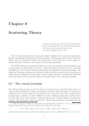
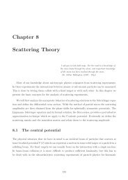
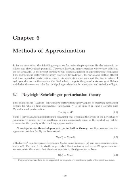
CHAPTER 6. METHODS OF APPROXIMATION 107Figure 6.2: Schematic diagram for the splitting of the 2p levels of a hydrogen atom as a functionof an external magnetic field B. For small B the degeneracy of the six 2p levels is completelyremoved, but as B becomes large the levels j = 3,m = 2 −1 and j = 1,m = 1 converge, so that2 2 2the degeneracy is only partially removed in the limit of very large B (Paschen-Back effect).C j m l ,m sm s = 1 2m s = − 1 2j = l + 1 2j = l − 1 2√l+m j +1/22l+1√l−m−j +1/22l+1√l−m j +1/22l+1√l+m j +1/22l+1with m j = m l + m s . For the two cases j = l ± 1 2 the matrix elements of S z thus become( 〈〈jlsm j |S z |jlsm j 〉 = C l±1 2jlsmm l ,+ 1 l , + 1 〈∣ + C l±1 2jlsm2 2m l ,− 1 l , − 1 )∣ ×2 2S z(C l±1 2∣m l∣jlsm,+ 1 l , + 1 〉+ C l±1 2∣2 2m l∣jlsm,− 1 l , − 12 2〉 ) (6.49)= ( ∣∣∣C l± 1 22m l∣ 2 ∣− ∣C l±1 ,+ 1 2m 2l∣ 2) = ± 2m j(6.50),− 1 2 2 2l + 1The energy shift induced by a weak external magnetic field is therefore∆Ejlm Z j= e⃗ [Bm j ± m ]j= eB2m e c 2l + 1 2m e c m j ·{ 2l+22l+1j = l + 1/22lj = l − 1/22l+1(6.51)The spin-orbit coupling already removes the degeneracy in j. From equation (6.51) we see thata weak external magnetic field in addition lifts the degeneracy in m j , thus explaining the namemagnatic quantum number. A level with given quantum numbers n and j thus splits into 2j +1distinct lines. As an example consider the 2p orbitals of the hydrogen atom. The 2p 3/2 level,with j = l + 1/2, splits into 4 levels according to m j = 3 2 , 1 2 , −1 2 , −3 2 with ∆EZ = eB2m ec m j · 4The 2p 1/2 levels split into two with m j = ±1/2 and ∆E Z = eB2m ec m j · 23(see figure 6.2).Strong field and Paschen–Back effect. In the case of very strong magnetic fields thespin-orbit term becomes (almost) irrelevant and the Zeeman term H Z forces the electrons intostates that are (almost) eigenstates of L z + 2S z = J z + S z . The total angular momentum J 2 is3 .

CHAPTER 6. METHODS OF APPROXIMATION 108hence no longer conserved, but we L 2 and S 2 commute with ĤZ so that we can use the originalbasis |nlm l 〉 ⊗ |sm s 〉 for the calculation. The fact that a strong magnetic field thus breaks upthe coupling between spin and orbital angular momentum and makes them into individuallyconserved quantities is called Paschen–Back effect.The energy shift due to the external magnetic field B is now easily evaluated as∆E Z nlsm l m s= eB2m e c (m l + 2m s ). (6.52)The magnetic field B does not remove the degeneracy of the hydrogenic energy levels in l andit removes the degeneracy in m l and m s only partially. Considering again the 2p level as shownin figure 6.2 we insert m l = −1, 0, 1 and m s = ±1/2 into equation (6.52). Due to the g-factorm l + 2m s can now assume all 5 integral values between ±2, but the value m l + 2m s = 0 canbe obtain in two different ways and hence corresponds to a degenerate energy level. In figure6.2 one observes that the m j = − 1 line originating from 2p 2 3/2 and the m j = 1 line originating2from 2p 1/2 converge for large B.The Stark effect. A hydrogen atom in a uniform electric field ⃗ E = E z ⃗e z experiences ashift of the spectral lines that was first observed in 1913 by Stark. The interaction energy ofthe electron in the external field amounts to an external potential V S = −e ⃗ E⃗x and hence to aninteraction HamiltonianH S = −e ⃗ E ⃗ X = −eE z z (6.53)First of all we shall assume that E is large enough for the fine structure effects to be negligible.We hence work in the basis |nlm〉 and ignore the spin because the electric field does not coupleto the magnetic moment of the electron. The matrix elements of H S are strongly constrainedby symmetry considerations. First we note that z is invariant under rotations about the z-axisso that J z is conserved and 〈l ′ m ′ |z|lm〉 is proportional to δ m,m ′. Moreover, under a paritytransformation ⃗ X → − ⃗ X the interation term H S is odd, so that〈l ′ m ′ |z|lm〉⃗x ↦→ −⃗x−→ (−1) l−l′ +1 〈l ′ m ′ |z|lm〉. (6.54)Since the integral ∫ d 3 x|ψ(⃗x)| 2 z is invariant under the change of variables ⃗x ↦→ −⃗x the matrixelement can be non-zero only if l − l ′ is odd. Moreover, one can show that |l − l ′ | ≤ 1 forthe electric dipole matrix element 〈| ⃗ X|〉, as we will learn in the context of tensor operators. 4Nonzero matrix elements therefore cannot be diagonal so that a linear Stark effect (i.e. acontribution in first order perturbation theory) can only occur if energy levels are degeneratefor different orbital angular momenta. Such degeneracies only occur for excited states of theHydrogen atom (in the ground state one can only observe the quadratic Stark effect, i.e. a levelsplitting in second order perturbation theory.The simplest situation for which we can hope for a linear Stark effect is for l = 0, 1 andn = 2, for which there may be a nonzero matrix element between |200〉 and |210〉, which aredegenerate and satisfy the selection rules l − l ′ = 1 and m = m ′ . Evaluation of the matrixelement yields〈210|z|200〉 = 〈200|z|210〉 = −3eE z a 0 , (6.55)4 A vector operator ⃗ X correponds to addition of spin 1. Adding spin one to a state of angular momentum lcan only yield angular momentum l ′ with |l ′ −l| ≤ 1 (see chapter 9). The same argument will apply to selectionrules of in the dipol approximation for absorption and emission of electromagnetic radiation (see section 6.5).

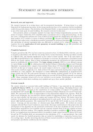
CHAPTER 6. METHODS OF APPROXIMATION 109Figure 6.3: Splitting of the degenerate n = 2 levels of hydrogen due to the linear Stark effect.where a 0 is the Bohr radius. Since a matrix of the form ( 0 λλ 0)has eigenvalues ±λ the levelshifts of the linear Stark effect in the hydrogen atom for n = 0, which affect the two states withmagnetic quantum number m = 0, are∆E S n=2,m=0 = ±3eE z a 0 . (6.56)as shown in figure 6.3. Recall that the linear Stark effect can only occur if there are degenerateenergy levels of different parity, which can only occur for hydrogen.6.4 The variational method (Riesz)The variational method is an approximation technique that is not restricted to small perturbationsfrom solvable situations but rather requires some qualitative idea about how the groundstate wave function looks like. It is based on the following fact:Theorem: A wave function |u〉 is a solution to the stationary Schrödinger equation if and onlyif the energy functionalE(u) = 〈u|H|u〉(6.57)〈u|u〉is stationary, i.e.H|u〉 = E|u〉 ⇔ δE = 0 (6.58)for arbitrary variations u → u+δu, where we do not normalize u in order to have unconstrainedvariations.For the proof of this theorem we compute the variation of the functional (6.57). Since variationsare infinitesimal changes they obey the same rules as differentiation, including the formula(f/g) ′ = f ′ /g − fg ′ /g 2 , i.e.δE = δ(〈u|H|u〉)〈u|u〉− (〈u|H|u〉)δ(〈u|u〉)(〈u|u〉) 2= δ(〈u|H|u〉)〈u|u〉− E δ(〈u|u〉)〈u|u〉 . (6.59)Using the product rule δ〈u|u〉 = 〈δu|u〉 + 〈u|δu〉 stationarity of the energy implies0 = ||u|| 2 · δE = 〈δu|H|u〉 − E〈δu|u〉 + 〈u|H|δu〉 − E〈u|δu〉. (6.60)If the variations of u and u ∗ can be done independently then the first two terms (and the lasttwo terms) on the r.h.s. have to cancel one another, i.e. 〈δu|H|u〉 − E〈δu|u〉 = 0, for arbitrary

CHAPTER 6. METHODS OF APPROXIMATION 110variations 〈δu| of u ∗ (⃗x), which is equivalent to the Schrödinger equation. To see that this isindeed the case we replace u by v = iu in (6.60) so that δv = iδu and δv ∗ = −iδu ∗ , implyingAdding i times (6.61) to (6.60) we find0 = −i ( 〈δu|H|u〉 − E〈δu|u〉 ) + i ( 〈u|H|δu〉 − E〈u|δu〉 ) . (6.61)δE = 0 ⇒ 〈δu|(H − E)|u〉 = 0 ∀ 〈δu|, (6.62)which implies the Schrödinger equation. This completes the proof since, in turn, (H −E)|u〉 = 0implies the vanishing of the variation (6.60).If we expand |u〉 in a basis of states |u〉 = ∑ n c n|e n 〉 then our theorem tells us that theSchrödinger equation is equivalent to the equations ∂E∂c n= 0. But for an infinite–dimensionalHilbert space we would have to solve infinitely many equations.The variational method thus proceeds by introducing a family of trial wave functionsu(α 1 ,α 2 ,...,α n ) (6.63)parametrized by a finite number of variables α i and extremizes the energy functional within thesubset of Hilbert space functions that are of the form (6.63) for some values of the parametersα i , i.e. we solve the∂E(u(α 1 ,...))∂α 1= ... = ∂E(u(α n,...))∂α n= 0. (6.64)If the correct wave function |u 0 〉 for the ground state happens to be contained in the family(6.63) of trial functions then the solution to the stationarity equations with the smallest value ofE(u) provides us with the exact solution to the Schrödinger equation. If we have, on the otherhand, a badly chosen family that does not anywhere come close to |u 0 〉 then our approximationto the ground state energy may be arbitrarily bad. Nevertheless, for an orthonormal energyeigenbasis |e n 〉〈u|H|u〉 = ∑ |c n | 2 〈e n |H|e n 〉 = ∑ |c n | 2 E n ≥ ||u|| 2 E min ⇒ E ≥ E min (6.65)so that we will always find an rigorous upper bound for the ground state energy.6.4.1 Ground state energy of the Helium atomWe now apply the variational method to improve a perturbative computation of the goundstate energy of the helium atom, which is a system consisting of a nucleus with charge Ze = 2eand two electrons. Treating the nucleus as infinitely heavy and neglecting relativistic effectslike the spin-orbit interaction we consider the HamiltonianH = − 22m e(∆ 1 + ∆ 2 ) − 2e2r 1− 2e2r 2+ e2r 12, (6.66)which consists of the kinetic energies T i = − 22m w∆ i , the Coulomb energies V i = −2e 2 /|⃗x i | dueto the attraction by the nucleus and the mutual repulsion V 12 = e 2 /|⃗x 1 −⃗x 2 | of the electrons. Ifwe omit the repulsive interaction among the electrons in a first step, the Hamiltonian becomesthe sum of two commuting operatorsH 0 = − 22m e(∆ 1 + ∆ 2 ) − 2e2r 1− 2e2r 2= (T 1 + V 1 ) + (T 2 + V 2 ) (6.67)

CHAPTER 6. METHODS OF APPROXIMATION 111for two independent particles and the Schrödinger equation H 0 |u〉 = E 0 |u〉 is solved by productwave functionsu(⃗x 1 ,⃗x 2 ) = u n1 l 1 m 1(⃗x 1 )u n2 l 2 m 2(⃗x 2 ) (6.68)The energy thus becomes the sum of the two respective energy eigenvalues,( 1E 0 = −Z 2 R + 1 ), (6.69)n 2 1 n 2 2where R = 2 /2m e a 2 0 = m e e 4 /2 2 = 13.6eV is the Rydberg constant. For the approximateground state wave function u pert0 (⃗x 1 ,⃗x 2 ) = u 100 (⃗x 1 )u 100 (⃗x 2 ) this implies E pert0 ≈ −108.8eVwhere the superscript refers to the Rayleigh–Schrödinger perturbation theory withH = H 0 + V,V = V 12 = e2r 12. (6.70)For the wave function we have ignored so far the spin degree of freedom and the Pauli exclusionprinciple. In chapter 10 (many particle theory) we will learn that wave functions of identicalspin 1/2 particles have to be anti-symmetrized under the simultaneous exchange of all of theirquantum numbers (position and spin), which is the mathematical implementation of Pauli’sexclusion principle. For the ground state of the helium atom the wave function is symmetricunder the exchange ⃗x 1 ↔ ⃗x 2 and total antisymmetry implies antisymmetrization of the spindegrees of freedom so thatu 0 (⃗x 1 ,⃗x 2 ,s 1z ,s 2z ) = u 100 (⃗x 1 ) u 100 (⃗x 2 ) |0, 0〉 12 , (6.71)where |0, 0〉 12 is the singlet state in spin space. Since this will not influence any of our resultswe will, however, ignore the spin degrees of freedom for the rest of the calculation.Taking into account now the repulsion term V between the electrons in (6.70) as a perturbation,the first order ground state energy correction becomes∫E 1 = 〈u 0 |V 12 |u 0 〉 = e 2 d 3 x 1 d 3 |u 100 (⃗x 1 )| 2 |u 100 (⃗x 2 )| 2x 2 (6.72)|⃗x 1 − ⃗x 2 |whereu 100 (⃗x) = √ 1 ( )3Z2− e Z r a 0π a 0(6.73)is the wave function of a single electron in the Coulomb field of a nucleus with atomic numberZ and a 0 is the Bohr radius.The integrals for the energy correction (6.72) are best carried out in spherical coordinates,( ) Z3 2 ∫ ∞E 1 = dra 3 1 r1e 2 −2Z0π0a 0r 1∫ ∞0dr 2 r 2 2e −2Za 0r 2∫dΩ 1 dΩ 2e 2|⃗x 1 − ⃗x 2 | . (6.74)If we first perform the angular integration dΩ 1 it is useful to recall that a spherically symmetriccharge distribution 5 at radius r 1 creates a constant (force-free) potential −q/r 1 in the interior5 Since all solutions to the homogeneous Laplace equation are superpositions of r l Y lm and r −l−1 Y lm sphericalsymmetry implies l = 0 so that the potential is constant in the interior r < r charge , as there is no singularity atthe origin, and proportional to 1/r for r > r charge , as the potential has to vanish for r → ∞.

CHAPTER 6. METHODS OF APPROXIMATION 113The virial theorem: If the potential V (⃗x) of a Hamiltonian of the formis homogeneous of degree n, i.e.H = T + V,T = P22m(6.83)then the expectation values of T and V are related by 6V (λ⃗x) = λ n V (⃗x) ∀ λ ∈ R, (6.84)2 〈u|T |u〉 = n 〈u|V |u〉 (6.88)so that 〈u|T |u〉 = n2E and 〈u|V |u〉 = E for every bound state |u〉.n+2 n+2Since the Coulomb potential is homogeneous of degree n = −1 we findT i = − 1 2 V i = Z 2 R = Z2 e 22a 0↦→ 〈u(b)|T i |u(b)〉 = b2 e 22a 0, 〈u(b)|V i |u(b)〉 = − bZe2a 0. (6.89)The energy functional E(b) = 〈u(b)| (T 1 + V 1 + T 2 + V 2 + V 12 ) |u(b)〉 thus becomesE(b) = e2a 0(b 2 − 2bZ + 5 8 b) = e2a 0((b − Z +516 )2 − (Z − 5 16 )2) . (6.90)The minimal value E min = e2a 0(Z − 516 )2 is obtained for b = Z − 5 . For the helium atom we16thus obtainE (var) (He= − e2 27 2a 0 16)≈ 77.5 eV, (6.91)which is only 2% above the experimental value (6.80). The effecitve charge becomes b ≈ 2716 .6.5 Time dependent perturbation theoryWe now turn to non-stationary situations. In particular we will be interested in the responseof a system to time dependent perturbationsH(t) = H 0 + W(t), (6.92)where the unperturbed Hamiltonian H 0 is not explicitly time dependent. For simplicity weassume that the unpertubed system has discrete and non-degenerate eigenstatesH 0 |ϕ n 〉 = E n |ϕ n 〉. (6.93)6 The proof of the quantum mechanical virial theorem is based on the Euler formula∑x i ∂ i V (⃗x) = nV (⃗x) (6.85)ifor a homogeneous potential of degree n and on the fact that the expectation value of a commutator [H,A]vanishes for bound states |u i 〉,The theorem then follows for A = ⃗ X ⃗ P because〈u i |[H,A] |u i 〉 = 〈u i |HA − AH|u i 〉 = 〈u i |E i A − AE i |u i 〉 = 0. (6.86)[ X ⃗ P, ⃗ P2 P22m] = 2i2m , [ X ⃗ P,V ⃗ ] = i Xi ∂ i V ⇒ [ X ⃗ P,H] ⃗ = i(2T − nV ). (6.87)For further details see, for example, chapter 4 of [Grau].

CHAPTER 6. METHODS OF APPROXIMATION 114If the perturbation is turned on at an initial time t 0 this impliesi ∂ ∂t |ϕ(t)〉 = H 0|ϕ(t)〉 for t < t 0 (6.94)i ∂ ∂t |ψ(t)〉 = (H 0 + W(t)) |ψ(t)〉 for t > t 0 (6.95)where the state |ψ i (t)〉 is defined by the initial condition|ψ i (t = t 0 )〉 = |ϕ i (t 0 )〉 (6.96)if the system is originally in the stationary state |ϕ i 〉. We first consider two limiting situations: In the sudden approximation we assume that a time independent perturbation isswitched on very rapidly,t switch ≪ t response ⇒ W(t) ≃ θ(t − t 0 )W ′ (6.97)so that we can describe the time dependence by a step function θ(t − t 0 ). A physicalexample would be a radioactive decay, where the reorganization of the electron shelltakes much longer than the nuclear reaction. Hence the Hamiltonian suddently changesto a new time-independent form H ′ = H 0 + W ′ . For t > t 0 the system has a new setof stationary solutions |ψ f 〉, and since the wave function has no time to evolve under atime-dependent force the transition probability into a final stateP i→f = |〈ψ f |ϕ i 〉| 2 (6.98)is determined by the operlap (scalar product) of the wave functions. The adiabatic limit is the other extremal situation,t switch ≫ t response , (6.99)for which the time variation of the external conditions is so slow that it cannot induce atransition and the system evolves by a continuous deformation of the energy eigenstatebecause we have, at each time, an almost stationary situation. More quantitatively, thetransition probability will be negligable if the energy uncertainty that is due to the timevariation of H is small in comparison to differences between energy levels.In the rest of this section we will consider small time-dependent perturbations W(t) = λV (t),where a small parameter λ can be introduced to control the perturbative expansion, but it isequivalent to simply count powers of W. Since the perturbation is small we can, at each instantof time at which we perform a measurement, use eigenstates |ϕ f 〉 of H 0 to represent the possibleoutcomes of the reduction of the wave function. Our aim hence is to determine the probabilityP i→f = |〈ϕ f |ψ i (t)〉| 2 (6.100)for finding the system in a final eigenstate |ϕ f 〉 after having evolved from |ϕ i 〉 under the influenceof H = H 0 +W according to (6.95) with boundary condition (6.96). For simplicity we set t 0 = 0.It is convenient to perform the perturbative computation of (6.100) in the interaction picture|ψ(t)〉 I = e i H 0t |ψ(t)〉 = U † 0(t)|ψ(t)〉, U 0 (t) = e − i H 0t , (6.101)so thati ∂ t |ψ(t)〉 I = W I (t)|ψ(t)〉 I with W I (t) = e i H 0t W(t)e − i H 0tas we found in (3.135–3.141).(6.102)

CHAPTER 6. METHODS OF APPROXIMATION 115Our next step is to transform the Schrödinger equation (6.102) of the interaction pictureinto an integral equation by integrating it over the interval from t 0 = 0 to t,|ψ i (t)〉 I = |ϕ i 〉 + 1i∫ t0dt ′ W I (t ′ )|ψ i (t ′ )〉 I , (6.103)where we used the boundary condition (6.96). For small W I (t) we can solve this equation byiteration, i.e. we insert |ψ i 〉 I = |ϕ i 〉+O(W) on the r.h.s. and continue by inserting the resultinghigher order corrections of |ψ i 〉 I . We thus obtain the Neumann series 7|ψ i (t)〉 = |ϕ i 〉}{{}initial stateThe transition amplitude now becomes+A i→f = 〈ϕ f |ψ i (t)〉 = δ if − i ∫ t+ 1 dt ′ W I (t ′ )|ϕ i 〉 +i 0} {{ }first order correction∫1 t ∫ t ′dt ′ dt ′′ W(i) 2 I (t ′ )W I (t ′′ )|ϕ i 〉 +... (6.106)0 0} {{ }second order correction∫ t0dt ′ 〈ϕ f | W I (t ′ ) |ϕ i 〉 + O(W 2 I ). (6.107)In the remainder of this section we focus on the leading contribution to the transition from aninitial state |ϕ i 〉 to a final state |ϕ f 〉 with f ≠ i,A (1)i→f= − i = − i ∫ t0∫ t0dt ′ 〈ϕ f | e i H 0t ′ W(t ′ )e − i H 0t ′ |ϕ i 〉 (6.108)dt ′ e i (E f −E i )t ′ 〈ϕ f |W(t ′ ) |ϕ i 〉 (6.109)where we used H 0 |ϕ i 〉 = E i |ϕ i 〉 and 〈ϕ f |H 0 = 〈ϕ f |E f to evaluate the time evolution operators.For first order transitions we thus obtain the probabilityP (1)i→f = 1 ∣∫ ∣∣∣ t2dt ′ e iω fit ′ 〈ϕ 2 f |W(t ′ )|ϕ i 〉∣(6.110)with the Bohr angular frequency0ω fi = E f − E i(6.111)Note that the transition probability (6.110) is related to the Fourier transform at ω fi of thematrix element 〈ϕ f |W(t ′ )|ϕ i 〉 restricted to 0 < t ′ < t.7 Introducing the time ordering operator T byTA(t 1 )B(t 2 ) = θ(t 1 − t 2 )A(t 1 )B(t 2 ) + θ(t 2 − t 1 )B(t 2 )A(t 1 ) ={A(t 1 )B(t 2 ) if t 1 > t 2B(t 2 )A(t 1 ) if t 1 < t 2(6.104)the Neumann series can be subsumed in terms of a formal expression for the time evolution operator|ψ i (t)〉 I = U I (t)|ϕ i 〉, U I (t) = Te − i R t0 dt′ W I(t ′ )(6.105)as is easily checked by expansion of the exponential.

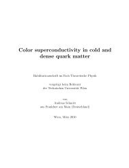
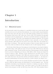
CHAPTER 6. METHODS OF APPROXIMATION 116|A ± | 2 ω−ω fiFigure 6.4: The functions |A ± | 2 = sin2 (∆ωt/2)(∆ω/2) 2ω fi→ 2πtδ(∆ω) of height t 2 /2 and width 4π/t.Periodic perturbations. In practice we will often be interested in the response to periodicexternal forces of the formW(t) = θ(t)(W + e iωt + W − e −iωt ) with W † − = W + . (6.112)Then the time integration can be performed with the resultP (1)i→f = 1 ∣ ∣∣ A+ 〈ϕ 2 f |W + |ϕ i 〉 + A − 〈ϕ f |W + |ϕ i 〉 ∣ 2 (6.113)in terms of the integralsA ± =∫ t0dt ′ e i(ω fi±ω)t ′ = ei(ω fi±ω)t − 1i(ω fi ± ω)= e i 2 (ω fi±ω)t sin ( (ω fi ± ω)t/2 )(ω fi ± ω)/2. (6.114)Figure 6.4 shows that the functions A ± (ω) are well-localized about ω = ∓ω fi , respectively, andconverge to δ-functions( ) 2|A ± | 2 = sin ∆ωt/2→ 2πtδ(∆ω) with ∆ = ω ± ω∆ω/2fi (6.115)for late times t ≫ 1/ω fi , where the prefactor follows from the integral∫ ( ) 2 ∞ dξ sin(tξ)−∞ ξ = πt ⇒ lim1t→∞ t( ) 2 sin(tξ)ξ = πδ(ξ). (6.116)For t → ∞ the interference terms between A + W + and A − W − in (6.113) can hence be negleted,P i→f→ 2πt(δ(E f − E i − ω) ∣ ∣〈f|W − |i〉 ∣ ∣ 2 + δ(E f − E i + ω) ∣ ∣〈f|W + |i〉 ∣ ∣ 2) (6.117)For frequencies ω ≈ ±ω fi the transition probabilities become very large so that the contributionof A − W − is called resonant term (absorption of an energy quantum ω fi ) while A + W + is calledanti-resonant (emission of an energy quantum ω fi ). Since the probability becomes linear in tit is useful to introduce the transition rateFor discrete energy levels we thus obtain Fermi’s golden ruleΓ i→f = lim t→∞ ( 1 t P i→f). (6.118)Γ i→f = 2π |〈f|W ±|i〉| 2 δ(E f − E i ± ω) (6.119)which was derived by Pauli in 1928, and called golden rule by Fermi in his 1950 book NuclearPhysics. The δ-function infinity for discrete energy levels is of course an unphysical artefact of

CHAPTER 6. METHODS OF APPROXIMATION 117our approximation. In reality spectral lines have finite width. For transitions to a continuumof energy levels we introduce the concept of a level density ρ(E) by summing over transitionsto a set F of final states,Γ i→F = ∑ ∫ ∫Γ i→f → df Γ i→f = dE ρ(E) Γ i→f (6.120)f∈Ff∈FInserting this into the golden rule we can perform the energy integration and obtain the integratedrateFΓ i (ω) = ρ(E f ) 2π |〈f|W ±|i〉| 2 , E f = E i ± ω. (6.121)If f ∈ F is characterized by additional continuous quantum numbers β, like for example thesolid angle covered by a detector, the level density can be generalized to df(E,β)=ρ(E,β)dE dβand the integrated transition rate is obtained by integrating over the relevant range of β’s.6.5.1 Absorption and emission of electromagnetic radiationWe now want to compute the rate for atomic transitions of electrons irradiated by an electromagneticwave. The relevant Hamiltonian can be written aswithWe split the Hamiltonian asH = 1 (P 2 − e A2m e c ⃗ ) 2 e + V (r) −2m e c ⃗σ B ⃗ (6.122)⃗A . . . vector potential of electromagnetic radiationV (⃗r) . . . central potential created by the nucleuse2m ecB . . . magnetic interaction with the radiation fieldand interaction termH = H 0 + W(t) with H 0 = P 2W B2m e+ V (r) (6.123)W(t) = −e2m e c (⃗ PA ⃗ + A ⃗ P) ⃗ − e2m} {{ } e c ⃗σ B ⃗ + e2A2m} {{ } e c ⃗2 . (6.124)2W AThe last term can be ignored because it is quadratic in the perturbation A. ⃗ For the vectorpotential of the electromagnetic field we take a plane wave)⃗A(⃗x,t) = ⃗ǫ A 0(e −i(ωt−⃗k⃗x) + e i(ωt−⃗ k⃗x)(6.125)with frequency ω and polarization vector ⃗ε. Since ⃗ B = curl ⃗ A = i ⃗ k × ⃗ A the magnetic interactionterm W B can be neglected for optical light, for which k ≪ |〈f| ⃗ P |i〉| ∼ /a 0 . In the radiationgaugediv ⃗ A = i ⃗ P ⃗ A = 0 ⇔ ⃗ε ⃗ k = 0 (6.126)

CHAPTER 6. METHODS OF APPROXIMATION 118⃗P ⃗ A + ⃗ A ⃗ P = 2 ⃗ A ⃗ P and the relevant matrix element becomes (up to a phase)e〈f|W A |i〉 = −A 0m e c ⃗ε 〈f|⃗ Pe ±i⃗k⃗x |i〉 (6.127)For optical transitions expectation values of ⃗x are of the order of a 0 ≪ 1/k so that we can dropcontributions from the exponential〈f| ⃗ Pe ±i⃗ k⃗x |i〉 ≈ 〈f| ⃗ P |i〉. (6.128)This is called electric dipole approximation because the matrix element of ⃗ P can be relatedto the matrix element of the dipole⃗D fi = 〈f| ⃗ X|i〉 (6.129)using[H 0 , ⃗ X] = im e⃗ P ⇒ 〈f| ⃗ P |i〉 = im e 〈f| [H 0, ⃗ X] |i〉 = i me (E f − E i )〈f| ⃗ X|i〉. (6.130)Inserting everything into Fermi’s golden rule we obtain the transition rateΓ i→f= 2π A 0 e m e ∣m e c (E f − E i )⃗ε 〈f| X|i〉 ⃗ 2∣ δ(E f − E i ± ω) (6.131)= 2πe2 ω 2δ(E c 2 f − E i ± ω)A 2 ∣0 ∣⃗ε 〈f| X|i〉 ⃗ ∣ 2 . (6.132)The selection rules for the dipole approximation are obtained by considering the matrixelements〈n ′ l ′ m ′ | ⃗ X|nlm〉. (6.133)Under a parity transformation ⃗ X → − ⃗ X the spherical harmonics transform asY lm (π − θ,ϕ + π) = (−1) l Y lm (θ,ϕ). (6.134)The matrix element (6.133) hence transforms with a factor (−1) l+l′ +1 so that spherical symmetryimplies that l − l ′ must be odd. Since[L z ,X 3 ] = 0, [L z ,X i ± iX 2 ] = ±(X 1 ± iX 2 ) (6.135)the components X 3 and X ± = X 1 ± iX 2 of X ⃗ change the magnetic quantum number bym ′ − m ∈ {0, ±1}. More generally, we will learn in the chapter 9 the vector operator X ⃗corresponds to addition of angular momentum 1, so that |l ′ − l| ≤ 1. Combining all constaintswe findl ′ − l = 1, −1, m ′ l − m l = 1, 0, −1. (6.136)Moreover, since we neglected magnetic interactions, spin in conserved m ′ s = m s . These selectionrules translate toj ′ − j = 1, 0, −1, j = 0 ⇒ j ′ = 1 (6.137)in the total angular momentum basis |jlsm j 〉.