Doppler sonar observations of Langmuir circulation - Jerry Smith's ...

Chapter 19DOPPLER SONAR OBSERVATIONS OF LANGMUIRCIRCULATIONJEROME A. SMITHScripps Institution of OceanographyLa Jolla, California19.1 Introduction19.2 The Data19.3 Bulk Models and LC scaling19.4 Results: Scaling of Surface Motion19.5 Conclusions19.6 Acknowledgements19.7 References19.1 IntroductionIt has become increasingly clear that air-sea coupling is important to the earth'sweather and climate [e.g., Grotzner et al. 1998, Xu et al. 1998]. The oceanic surfacemixed layer is the link by which the air and sea are coupled. Further, the form andstrength of the mixing motion are important to important concerns such as the fluxesof gases and nutrients and the growth and health of marine life. Improved understandingof all these processes depends in some measure on our understanding mechanisms anddynamics of the mixed layer.One-dimensional “slab-models” of the mixed layer have performed remarkably well[e.g., Pollard et al. 1973, Price et al. 1986, O'Brien et al. 1991, Large et al. 1994, Li etal. 1995]. Under active mixing, the oceanic density profile erodes from the surfacedownward, producing a uniform layer over the remaining deeper profile. This mixedlayer is approximately uniform in both velocity and density, with “jumps” occurring inboth at the relatively sharp thermocline at the layer’s base (like a “slab”). Horizontalgradients are assumed a priori to be of secondary importance. The erosion rate is thenset to maintain a threshold value of the bulk Richardson number, depending only on thedepth of the layer and the jumps in velocity and density at the base [Pollard, et al.1973]. Some additional improvement is attained by permitting the erosion to penetratesmoothly into the thermocline over a depth proportional to the total mixed layer depth[Large, et al. 1994]. Additional deepening occurs when water at the surface is madedenser by surface buoyancy fluxes; conversely, restratification occurs when heating539G. L. Geernaert (ed.), Air-Sea Exchange: Physics, Chemistry and Dynamics, 539-555.© 1999 Kluwer Academic Publishers. Printed in the Netherlands.)

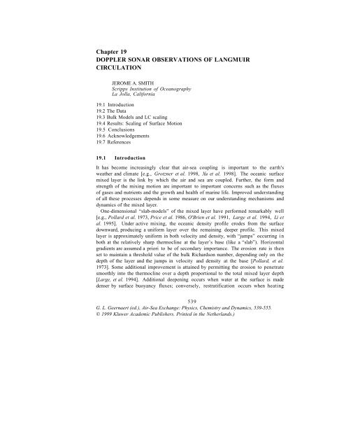
540 JEROME A. SMITHIntensity (±10 dB)Velocity (±20 cm/s)40003/09/95 2245:02 UTC3503002502000 50 100 150 200Distance E-W (m)0 50 100 150 200Distance E-W (m)Figure 19.1 Example frame of PADS data: (left panel) Acoustic backscatter intensity; (right)Radial velocity. The arrows indicate wind speed and direction; the arrow shownrepresents a 15 m/s wind. North is up. The data are smoothed to 3 minute averages,modified to “track” the mean flow across the area.exceeds mixing [Price, et al. 1986]. The velocity jump at the base of the mixed layercomes from inertial currents generated by the wind stress. Thus, while this bulk-shearmechanism is responsible for dramatically rapid initial deepening, it drops off near aquarter of an inertial day after the onset of wind, or in locations where inertial currentsare suppressed.Surface stirring by wind and waves can cause continued slower erosion [Niiler andKrauss 1977], and inhibits restratification. In its simplest form, the surface stirring isparameterized by a power of the wind friction velocity u*; however, the multiplier bestfitting the data varies from site to site. It is of interest to note two cases where thesesimple models deviate from the data: (1) [O'Brien, et al. 1991] note the failure of the realmixed layer to restratify as quickly as the model immediately after a rapid drop in wind;(2) Li, et al. [1995] note a tendency for the mixed layer depth to continue increasingslightly faster than the model with sustained winds. Li, et al. [1995, also Li and Garrett1997] suggest that Langmuir circulation is responsible for the continued erosion, sodeepening should depend on a combination of wave Stokes’ drift and wind stress, assuggested by recent theories and models for the forcing of Langmuir circulation. Wherewaves are nearly fully developed the waves and wind is tightly coupled. In this case,scaling by the combined wind-wave term can be hard to separate statistically from justwind stress scaling (provided the magnitude of this stirring term is adjusted for thetypical waves there). Notably, however, there are both places and times when therelation between wind and waves is not so direct. In particular, the anomalous mixingin “case 1” above occurs during a time of large waves and small stress, intimating thatwaves play an important role. It is suggested that wave climate variations cause the“stirring parameter” to vary.Observations of the mixed layer often reveal coherent structures. These invitemodeling with simplified dynamics, with hope of understanding their existence,behavior, and mixing efficiency. One such structure consists of horizontal rolls having

542 JEROME A. SMITHis friction velocity and U s the surface Stokes’ drift due to the waves. However, as weshall see, the observations indicate that the surface velocity V scales with U s alonewithin each well defined "wind event," once Langmuir circulation is established. Theconstant of proportionality varies significantly from one event to another, so thatblindly averaging over several events destroys the correlation. This scaling suggeststhat (1) fully developed (nonlinear) Langmuir circulation does not scale the same way asinitial growth, and (2) some additional variable is needed to parameterize this motion.19.2 The Data.Data from 2 field experiments are considered: the “Surface Waves Processes Program”(SWAPP), which took place some 300 km West of Pt. Conception, CA, in March of1990, and leg 1 of the “Marine Boundary Layer Experiment (MBLEX), which took place50 to 100 km offshore and just North of Pt. Conception (Figure 19.2). The former wasundertaken with FLIP in a 3-point deep-ocean mooring, while in the latter FLIP waspermitted to drift freely with the upper 90 m of the water column. In both, the surfacevelocities are estimated from surface-grazing acoustic Doppler sonar systems. InSWAPP, 4 discrete “inverted side-scan” style beams were used to trace the time-spaceevolution of features along 4 directions, distributed at 45° increments. In MBLEX, anewer system (PADS) was used to image a continuous area 35° in bearing by 450 m inrange. Details concerning the former are found in [Smith 1992] and concerning thelatter in [Smith 1998].Wind and Stokes’ drift are primary input parameters for models of Langmuircirculation. In both experiments, wind stress was estimated from sonic anemometerdata via eddy-correlation methods. Stokes’ drift was derived using data from resistancewirewave arrays, yielding surface elevations and tilts as functions of frequencies up to0.5 Hz [Longuet-Higgins et al. 1963]. The results are converted to Stokes’ drift vialinear theory and integrated over the directional-frequency spectrum to estimate the netdrift at the surface. Additional details concerning instrumentation for SWAPP may befound in [Smith 1992], and for MBLEX in [Smith 1998]. The wind and Stokes’ drift forMBLEX-1 are shown in Figure 19.3; those for SWAPP are shown in Figure 19.4.MBLEX-1 provided only one clear storm event. In SWAPP, 5 time segments wereidentified as encompassing potentially useful wind events. However, of these only thesecond and third segments have both steady wind directions and a wide range of waveage (segments are delineated in Figure 19.4 by different shades of gray; also denoted bythe symbols * and + below the peaks in Stokes’ drift).

DOPPLER SONAR OBSERVATIONS OF LANGMUIR CIRCULATION 54340°N3000San Francisco100040002000MBLEX-235°NSWAPPMBLEX-1Pt. ConceptionSanDiego1000400030°N125°W 120°W 115°WFigure 19.2 Locations of SWAPP and MBLEX experiments, showing (in particular) FLIP’sdrift-track over the most significant storm event in MBLEX-1.300020002000From (°T) Stokes(cm/s),Wind(m/s)20151050300250200150MagnitudesDirections10067 67.5 68 68.5 69 69.5Year Day 1995 (UTC)Figure 19.3 Wind (solid curve) and Stokes’ drift (dashed curve) over the focus time segmentof MBLEX leg 1. Note the delay between the onset of wind and development ofStokes’ drift. Just prior to this segment, the wind was from the NW, and swellcontinued to come from that direction, explaining the slow reversal in Stokes' driftdirection. Similar data were gathered for the SWAPP experiment.

544 JEROME A. SMITH2.5Friction Velocity (u*)1.5010Stokes Drift (Us)508642Vrms60 65 70Yearday 1990, UTCFigure 19.4 Wind, waves, and rms surface velocity during SWAPP. The first segment hasweak variable winds; the last segment contains several directional shifts; the secondto-lastsegment has little variation in the ratio U s /u*. Thus, only the second and thirdsegments are suitable for testing the relationship between the three parameters.Stratification and the shear across the pycnocline are also primary input parameters tosimple mixed layer models. In both experiments, stratification was monitored withrapid-profiling “Conductivity – Temperature – Depth” (CTD) systems, providingtemperature and salinity profiles to 400 m depth every couple minutes. One usefulsummary parameter is the mixed layer depth “h,” as shown (for example) in Figure 19.5for the MBLEX data set. Vertical profiles of horizontal velocity were monitored withadditional Doppler sonar systems in a standard Janus configuration. To estimate a “bulkshear,” the surface velocities estimated from the surface sonar systems were used,together with velocity estimates averaged over a sub-thermocline depth interval of thestandard Janus-type data.19.3 Bulk Models and LC scaling.To set the context for the following analysis of surface motion, and to help interpretthe results, it’s useful to review some simple ideas about wind mixing of the surfacelayer of an ocean. The MBLEX-1 event will be used for illustration. In the open ocean,

DOPPLER SONAR OBSERVATIONS OF LANGMUIR CIRCULATION 545the largest effect is the shear across the thermocline, parameterized by a bulkRichardson number,∆ρghRi ≡ ≥064. , or ∆ρ≥ 064 . ( ∆U) 2( ρ gh)ρ 0 ( ∆U)2o (19-1)[Pollard, et al. 1973, Price, et al. 1986]. The velocity jump across the thermocline ∆Uis primarily due to inertial currents generated by sudden changes in the wind; ittherefore generally decreases rapidly after a quarter inertial cycle. The time history ofthe strength of this term is indicated in Figure 19.6 (thickest line) in terms of the ∆ρneeded across the thermocline to halt mixing (i.e., for the measured ∆U and mixed layerdepth h). As shown in Figure 19.6 (thickest line), this term gets big quickly and thendecays almost to zero over the next day. Since the wind rose gradually over the firstday, the inertial currents were not as large as would have happened with a sudden windturn-on. This is the essential explanation for the shallowness of the mixed layer inMBLEX-1, in spite of apparently strong forcing: the inertial current turned past 90°0well before the maximum winds were reached.51015Depth (m)20253035404567 67.5 68 68.5 69 69.5 70Year Day 1995Figure 19.5 The mixed layer depth over the MBLEX-1 wind event, evaluated as the depth atwhich the temperature falls to 0.05°C below the value nearest the surface. The thinline shows “raw” mixed layer depth; the thick line is a psuedo-mixed-layer-depthfrom temperatures rescaled to constant heat capacity, compensating in part forvertical straining by low-mode internal waves or quasi-geostrophic motion.After fast deepening by the PRT mechanism, surface stirring by wind and waves servesto maintain the mixed layer against restratification, and can also effect continued slowdeepening [Niiler and Krauss 1977, Li, et al. 1995]. The parameterization of Li et al.incorporates scaling arguments appropriate to Langmuir circulation (i.e., a combination

546 JEROME A. SMITH10 0 Year Day 1995 (UTC)10 -10.65 |∆U| 2 / gh 50(u*) 2 ρ /gh9.8(U s u* 2 ) 2/3 ρ /ghσ Tunits10 -24V 2 ρ / gh67.5 68 68.5 69Figure 19.6 Mixing strength, parameterized by the density jump required to stop mixing, for (1)the bulk Richardson (or PRT) mechanism (thick line); (2) Langmuir circulation, asestimated directly from the rms velocity scale V (medium line); and (3) LC mixingestimated from U s and ν t via comparison with numerical model results, fordeveloping waves (thin solid line) and for fully developed waves (thin dashed line).of wind and wave velocity scales), although in the end they reduce the argument to asimple u* dependence by assuming fully developed seas. For the sake of discussion,this latter parameterization is conceptually extended to underdeveloped waves.The scaling suggested by Li et al. begins with the argument, derived from numericalmodeling, that penetration into the thermocline is stopped if∆ρ ≥ 123 . wdn 2 ( ρo gh), (19-2)where w dn is the maximum downwelling velocity associated with the Langmuircirculation. Using model results for w dn , they rewrite this in the form∆ρ ≥ Cu* 2 ( ρ gh)(19-3)owhereC≡ 036 . Uskν t , (19-4)in which ν t is the turbulent kinematic eddy viscosity and k is the wavenumber of thedominant surface waves. For fully developed seas, they argue C is about 50 (Figure19.6, thin dashed line). For illustration, this criterion is evaluated two additional ways:(1) extending the evaluation of C to underdeveloped waves, using estimates of U s , k,

DOPPLER SONAR OBSERVATIONS OF LANGMUIR CIRCULATION 547and ν t in (19-4), and (2) using the rms horizontal scale (as described in next section) toestimate w dn directly for use in (19-2).To pursue the underdeveloped case, a significant requirement is estimation of ν t .Recent dissipation measurements near the surface indicate that the turbulent velocityscale q is reasonable well described by the energy dissipation rate of the waves [Terrayet al. 1996]. This, in turn, is well estimated by the energy input to the waves (within7% or so). The growth rate β of a wave of radian frequency σ and phase speed c isapproximately β = 33σ( u*/ c ) 2 [Plant 1982], so the net energy flux can be written inthe formq 3 ∝ ρ−1 βE = 33ga 2 σ( u*/ c) 2 = 33( U s u* 2 ). (19-5)Conveniently, the final form in (19-5) remains approximately unchanged withintegration over the wave spectrum (within a factor representing the typical directionalspread). The length scale appropriate to wave breaking is proportional to the waveamplitude a, so we obtain an estimate of ν t of the form νs t ∝ aU ( u* 2 ) 1/3 . Substitutingthis into (19-4), and noting that ak in general does not vary significantly from about0.1, we obtainC∝Uskν t ∝( Usu*) 2/3 (19-6)The values employed by Li et al. [1995] for fully developed waves imply U s /u* → 11.5.To obtain 50 with this value in (19-3), the constant of proportionality is set to 9.8.Then (19-6) becomes∆ρ ≥ 98 .( Usu*) 2 2/3( ρo gh). (19-7)This criterion is also shown in Figure 19.6 (thin solid line).To use the measured V rms directly, we need to convert the horizontal rms to anestimate of maximum downwelling. Since the spacing is generally about twice themixed layer depth, the rolls are roughly isotropic in the crosswind plane, and it’sreasonable to set the vertical and crosswind velocity scales equal. Then the rms valuesmust be translated into estimates of the maximum downwelling velocities. Thecirculation is not simply sinusoidal (in which case wmax ~ 2 1/2 V) but varies somewhatrandomly. By analogy to estimating significant wave height from the rmsdisplacement, we set a threshold exceeded by 1/3 of all downwelling local maxima.This leads to a value roughly 2 times the rms. Hence we substitute 4V 2 from theempirical rms velocity assessment (section 19.4) for w dn in 2, as the direct estimate ofthe strength of mixing due to the observed Langmuir cells (Figure 19.6, lowest line).The mixing effect estimated from the surface velocity measured in MBLEX-1 fallsbelow the parametric estimates 3 and 7. As we shall see, the discrepancy is similar thatbetween the observed velocity scales; the SWAPP variances agree more closely withthese parameterizations. Over a period of several days, these differences could lead to

548 JEROME A. SMITHsignificant differences in the mixed layer depth. It is therefore important to understandhow and why this variance is reduced.19.4 Results: Scaling of Surface Motion.The features observed at the surface can be characterized in terms of strength, spacing,orientation, and degree of organization. The objective here is to see whether thepreviously observed scaling for the strength (rms velocity) holds up over the combineddata set. A subsidiary interest is to note the extent and limits to which intensityfluctuations compare to those of the dynamically more important velocity: canintensity images be used as a proxy for velocity in characterizing some aspects of theflow?To estimate time series of the strength of variations in both intensity and radialvelocity associated with Langmuir circulation, data averaged over 1 to 3 minutes wereemployed. The MBLEX-1 (PADS) data were averaged with a moving window that tracksthe mean advection across the imaged area as the average is formed (see [Smith 1998]for details). The SWAPP data were processed with a dual spatial-temporal lag techniqueto isolate coherent signals while also tracking advection along the beam (see[Plueddemann, et al. 1996] or [Smith 1996] for details). The data were corrected for thespatial response of the instruments, estimated from simulated data. Strength is gaugedby rms values. For radial velocity, the results are expressed in cm/s and denoted V. Forintensity I they are expressed in rms decibels (dB). Log-intensity relative to the mean,corrected for beam pattern and attenuation, is used for two pragmatic reasons: (1) itmakes the result independent of source loudness, and (2) the log-intensity is morenearly normally distributed, and so has better-behaved statistics.Timeseries of intensity and velocity strengths for the MBLEX-1 event are shown inFigure 19.7. Both wind speed W and Stokes’ drift U s are also shown, scaled byconstants chosen to yield reasonable fits to the rms velocities over the middle sectionof the time period. Streaks are first seen sometime after year day 67.7, as the windexceeds 8 m/s. It is therefore reasonable to restrict the scaling analysis to the timesegment after this. The strength scales of surface radial velocity features (or intensity)follow the Stokes’ drift quite closely from year day 67.7 to the end of the segment, i.e.,for winds over 8 m/s. The ratio of rms radial velocity (cm/s) to rms intensity (dB)remains close to 1.5 over the whole 44-hour period, indicating that similar informationis obtained from either with respect to gross strength. Note, however, that near the end,when the wind suddenly drops (and veers momentarily by 60°), the intensity strengthscaledrops by a larger fraction than velocity.In the absence of wave forcing, the only relevant velocity scale would be the wind W(or friction velocity u*; for present purposes, these are roughly proportional). Basedon theories for initial growth of Langmuir circulation, it has been suggested that thecross-wind velocity fluctuations should scale roughly with either the geometric mean ofthe wind and Stokes’ drift, (WU s ) 1/2 [Plueddemann, et al. 1996] or with (W 2 U s ) 1/3

DOPPLER SONAR OBSERVATIONS OF LANGMUIR CIRCULATION 54954.54Dark Symbols=VelocityLight Symbols=IntensitySolid = 0.25 Stokes' DriftDashed = 0.2%W=1.5u*Dotted = 0.3(U s u*) 1/2cm/s or dB3.532.521.510.5067.5 68 68.5 69Year Day 1995 (UTC)Figure 19.7 RMS radial velocity (dark symbols) and intensity (light symbols) associated withthe features, versus time. Each symbol represents a half-hour average; crossesrepresent dubious estimates, circles more reliable ones. For scaling and comparison,0.25U s (solid line), 0.002W (dashed line), and 0.023(U s W) 1/2 (dotted line) are alsoshown.[Smith 1996]. The suggested scalings for the surface velocity associated with Langmuircirculation can be cast in the general form V ~ u* (U s /u*) n . The value of n is then soughtas the slope of the best fit line to log 10 (V/u*) versus log 10 (U s /u*). The results forMBLEX-1 are reviewed in Figure 19.8; points where no surface stripes are visible aremarked with +’s and excluded from the fit. Surprisingly, the value n=1 was found, withlittle uncertainty (r 2 =0.89; error bounds on the slope are a standard deviation derived bythe bootstrap method with 5000 trials, cf. [Diaconis and Efron 1983]). Note that U s /u*varies over almost an order of magnitude, and. In other words, once the Langmuircirculation is well developed, V~U s , and wind stress no longer enters directly in scalingthe motion. This implies a strong influence of the waves on the flow (and nonlinear,since a threshold must be applied for the existence of well-developed Langmuircirculation).A natural question is whether this applies to other data, or is an isolated case. To thisend, the SWAPP data were reanalyzed. Figure 19.4 shows the time-histories of wind,waves, and measured surface velocity scale from SWAPP. Figure 19.9 shows the log-logplot for all SWAPP and MBLEX data points, without regard for the existence of stripesor non-stationary conditions. It would be easy to dismiss any correlation from thisplot; however, it should be recognized that (1) the parameter U S might be a proxy foranother wave parameter, and the relation between these might vary between windevents, and (2) there could be another parameter (or parameters) influencing the

550 JEROME A. SMITHrelation. It is wise to examine the relation on a case-by-case basis, to see if there is a“hidden” relation. Unfortunately, as noted above, only events 2 and 3 of the potential5 segments from SWAPP provide both a “clean” wind event (not confused by windveering) and a wide range of U S /u*. These two events (henceforth “SWAPP-2” and“SWAPP-3”) are plotted together with the “MBLEX-1” event in Figure 19.10. Theseregressions support the value n=1 for the exponent. Although the fits are not as tightas for the MBLEX-1 data, they are still statistically significant at well over 95%.Intriguingly, there is considerable offset between the lines, especially between SWAPPand MBLEX (by a factor of about 5), but also between the two SWAPP events (by afactor of about 2). Some other aspect of the environment must be affecting the relation.What could be responsible for the observed variation in velocity scale V rms ? Possiblecandidates include variations of scaled depth of the mixed layer kh, effective viscosityν t , a directional effect of the horizontal Coriolis component [Cox and Leibovich 1997],or suppression by the buoyancy of the near-surface bubble cloud. A summary of somerelevant parameters is given in Table 19.1. The first 6 parameters summarize theobservations for the 3 events; the rest are derived from these. An effective wave periodT S is derived from the surface Stokes’ drift, assuming the variations in mean-squarewave steepness are not very large:9Red crosses: no LCBlack circles: LC identified5V rms /u*21Slope = 1.001 ±0.034r2 = 0.8860.52 5 10U s 20/u*Figure 19.8 Scaling of the rms measured radial surface velocity takes the general formV~u*(U s /u*) n . The value of n is sought as the slope of (V/u*) versus (U s /u*) on alog-log plot. This figure indicates a well-determined value for n very near 1.0; i.e.,V ~ U s , with no dependence on u* once Langmuir circulation is well formed.Values before year day 67.66, when there were no signs of Langmuir circulation,are shown as red crosses but not included in the fit.

DOPPLER SONAR OBSERVATIONS OF LANGMUIR CIRCULATION 551V rms /u*10 110 0Us/u*10 0 10 1Figure 19.9 All data points from SWAPP and MBLEX-1, plotted without regard to event orwhether LC features were identified. No correlation is seen, and it appears thatalmost an order of magnitude uncertainty in V rms must be tolerated.slope = 1.001, r 2 = 0.886slope = 0.940, r 2 = 0.473slope = 1.148, r 2 = 0.664Vrms/u*10 110 0Us/u*10 0 10 1Figure 19.10 The empirical fits for n for each “good event” treated separately. Note that,within each event, the fit is fairly tight. However, the vertical offset of the linesvaries significantly over just these three events.

552 JEROME A. SMITHU S 1 ≈ ( ak) 2c p = T ( ak) 2g / 4π ≈( const.)T(19-8)2For the SWAPP-3 event, the peak wave period was estimated in a variety of ways[Bullard and Smith 1996], leading to a favored value of about 11.5 s near the end of theevent; thus, we set the value of (ak) 2 by matching to that value in that event. Thecorresponding value for (ak) 2 is 0.0084, well within reason. The effective wavenumberis then computed from T S via linear dispersion: ks= ( 2π/ Ts) 2 / g. Given theuncertainty in defining a “peak period,” and given the purported importance of waveStokes’ drift to the generation of Langmuir circulation, this proxy for the wave periodand length scales appears to be most appropriate.As reported in Table 19.1, the directions of MBLEX-1 and SWAPP-2 are similar, butthe V-scaling differs by the largest ratio. This appears to rule out both the opposingswell and the horizontal Coriolis hypotheses. The estimated wave-induced viscosity islargest for SWAPP-3, but this is intermediate in V-scaling. Another possibility issuppression of motion by bubble buoyancy. The level of breaking presumably sets theoverall density of the near surface bubble-cloud. A likely indicator of this is set bymatching the rise-rate of the largest bubbles to the wave breaking turbulent velocityscale (as discussed above in connection with the turbulent eddy viscosity). Comparingthis with the observed velocity scaling, it is seen that this parameter at least has theright ordering in magnitude, although the MBLEX-1 and SWAPP-3 values are relativelyclose. Finally, there is the “scale depth” kh of the mixed layer. It is important todistinguish here between the development of ∆V, V rms , h, U S , and k over the course of anevent versus the differences between events. These all develop in parallel over thecourse of a wind event; however, what is of interest at the moment is whether theydevelop either at different rates or from different initial values between events. It isthese latter differences between events that presumably set the ratio of V rms to U S overthe event. Thus it is emphasized that this “scaled depth” refers to final or quasiequilibriumvalues of h and k S .One way the scaled depth could influence the result is that the layer-averagedconvergent force should be subtracted from the surface value, since this works todepress the thermocline rather than drive circulation. For roughly exponential decaywith the depth-scale of the Stokes’ drift, this leads to a net force at the surface reducedby the factor01 −2kz−1 −2khF′ = F0−F ≈1− ∫ e dz = 1−( 2kh) ( 1−e)h(9)−hNote that this varies smoothly from 0 at kh=0 to 1 as kh gets large; in other words, thewind-wave forcing mechanism is reduced for very thin layers, and reaches the fullpredicted strength as the mixed layer becomes deeper than the wave’s scale-depth. Asseen, the effect is in the right direction, but is again too weak to explain the fulldifferences observed between the three events. It appears that further investigations areneeded to select between the alternatives and to determine why and when suppression ofthe motion occurs.

DOPPLER SONAR OBSERVATIONS OF LANGMUIR CIRCULATION 553Table 19.1 Various parameters that may influence the surface velocity scale.19.5 ConclusionsEvent MBLEX-1 SWAPP-2 SWAPP-3ParameterV rms /U S 0.25 0.95 0.67W dir SE SSE NNWW max 15 m/s 10 13.6u* 1.65 cm/s 1.1 1.5U S 7.0 cm/s 4.5 7.5h 25 m 25 45T S 10.7 s 6.9 11.5k S 0.035 m -1 0.085 0.031k S h 0.87 2.12 1.37F’ 0.53 0.77 0.66(u* 2 U S ) 1/3 0.124 cm/s 0.082 0.119ν t 698 cm 2 /s 190 770The rms velocities associated with the low-frequency features appear to scale tightlywith the Stokes’ drift alone over the course of individual wind events, rather than withthe wind or a combination of wind and waves. This relation is nonlinear in the sensethat a threshold must be set for the existence of Langmuir circulation before it holds.Further, the “constant of proportionality” between surface velocity variance andStokes’ drift varies significantly between events. It is suggested that this is related tothe ratio of wavelength to mixed layer depth, as parameterized by the “final” ormaximal values. Dynamic effects of the near-surface bubble layer could also play a role.In each event considered here, the mixed layer deepened rapidly, then remained fairlyconstant, with very slow (if any) continued erosion. This is consistent with currentthinking, where the “bulk dynamics” of shear across the thermocline due to inertialmotion is the primary agent for deepening in the open ocean. Surface stirring by thecombined action of wind and waves may help maintain the mixed layer after this, andmay induce additional slow deepening. In any case, the inertial current “bulkRichardson number” mechanism is the lowest order term in wind-induced mixing of thesurface layer.Overall strength correlates well between intensity and velocity features over longertimescales. However, in details such as spacing, orientation, or short-time behavior,significant differences occur. The time/space-dependent behavior of bubbles in a timevaryingflow should be investigated. Simulations with realistic bubble dynamics mayhelp to understand these differences.19.6 Acknowledgments.Thanks are due to the many people involved in both SWAPP and MBLEX. Regardingthe gathering of this data, thanks go especially to Eric Slater, Lloyd Green, MikeGolden, Chris Neely, R. Pinkel, K. Rieder, M. Alford, and to the crew of the researchplatform Flip, captained by E. DeWitt (SWAPP) and T. Golfinas (MBLEX). Thanks also

554 JEROME A. SMITHfor useful comments from R. Pinkel, C. Garrett, and G. Terray. This work was supportedby the Office of Naval Research, grants N00014-93-1-0359 and N00014-96-1-0030.ReferencesBullard, G. T., and J. A. Smith, Directional spreading of growing surface waves, in The air-seainterface: radio and acoustic sensing, turbulence and wave dynamics, Edited by M. A. Donelan,W. H. Hui, and W. J. Plant, pp. 311-319, The Rosenstiel Scholl of Marine and AtmosphericScience, Miami, FL, 1996.Cox, S. M., and S. Leibovich, Large-scale three-dimensional Langmuir circulation, Physics of Fluids,9, 2851-2863, 1997.Craik, A. D. D., The generation of Langmuir circulation by an instability mechanism, J. Fluid Mech.,81, 209-223, 1977.Craik, A. D. D., and S. Leibovich, A rational model for Langmuir circulations, J. Fluid Mech., 73,401-426, 1976.Diaconis, and B. Efron, Computer-intensive methods in statistics, Sci. Am., 248, 116-130, 1983.Farmer, D., and M. Li, Patterns of bubble clouds organized by Langmuir circulation, J. Phys.Oceanogr., 25, 1426-1440, 1995.Garrett, C., Generation of Langmuir circulations by surface waves– A feedback mechanism, J. Mar.Res., 34, 117-130, 1976.Grotzner, A., M. Latif, and T. P. Barnett, A decadal climate cycle in the North Atlantic Ocean assimulated by the ECHO coupled GCM, Journal of Climate, 11, 831-847, 1998.Langmuir, I., Surface motion of water induced by wind, Science, 87, 119-123, 1938.Large, W. G., J. C. McWilliams, and S. C. Doney, Oceanic vertical mixing: A review and a modelwith a nonlocal boundary layer parameterization, Rev. Geophys., 32, 363-403, 1994.Leibovich, S., Convective instability of stably stratified water in the ocean, J. Fluid Mech., 82, 561-581, 1977.Leibovich, S., On wave-current interaction theories of Langmuir circulations, J. Fluid Mech., 99,715-724, 1980.Li, M., and C. Garrett, Mixed layer deepening due to Langmuir circulation, J. Phys. Oceanogr., 27,121-132, 1997.Li, M., K. Zahariev, and C. Garrett, Role of Langmuir circulation in the deepening of the oceansurface mixed layer, Science, 270, 1955-1957, 1995.Longuet-Higgins, M. S., D. E. Cartwright, and N. D. Smith, Observations of the directional spectrumof sea waves using the motions of a floating buoy, in Ocean Wave Spectra: Proceedings of aConference, Edited by National Academy of Sciences, pp. 111-132, Prentice-Hall, EnglewoodCliffs, N.J., 1963.Niiler, P. P., and E. B. Krauss, One-dimensional models of the upper ocean, in Modeling andPrediction of the Upper Layers of the Ocean, Edited by E. B. Krauss, pp. 143-172, Pergammon,Tarrytown, N. Y., 1977.O'Brien, M. M., A. Plueddemann, and R. A. Weller, The response of oceanic mixed layer depth tophysical forcing - modelled vs observed, Biol. Bull., 181, 360-361, 1991.Plant, W. J., A relationship between wind stress and wave slope, J. Geophys. Res., 87, 1961-1967,1982.Plueddemann, A. J., J. A. Smith, D. M. Farmer, R. A. Weller, W. R. Crawford, R. Pinkel, S. Vagle,and A. Gnanadesikan, Structure and variability of Langmuir circulation during the surface wavesprocesses program, J. Geophys. Res., 101, 3525-3543, 1996.Pollard, R. T., P. B. Rhines, and R. Thompson, The deepening of the wind-mixed layer, Geophys.Fluid Dyn., 4, 381-404, 1973.Price, J. F., R. A. Weller, and R. Pinkel, Diurnal cycling: Observations and models of the upperocean response to diurnal heating, cooling, and wind mixing, J. Geophys. Res., 91, 8411-8427,1986.

DOPPLER SONAR OBSERVATIONS OF LANGMUIR CIRCULATION 555Smith, J. A., Observed growth of Langmuir circulation, J. Geophys. Res., 97, 5651-5664, 1992.Smith, J. A., Observations of Langmuir circulation, waves, and the mixed layer, in The Air SeaInterface: Radio and Acoustic Sensing, Turbulence, and Wave Dynamics, Edited by M. A.Donelan, W. H. Hui, and W. J. Plant, pp. 613-622, Univ. of Toronto Press, Toronto, Ont., 1996.Smith, J. A., Evolution of Langmuir circulation during a storm, Journal of Geophysical Research,103, 12,649-12,668, 1998.Smith, J. A., R. Pinkel, and R. Weller, Velocity structure in the mixed layer during MILDEX, J. Phys.Oceanogr., 17, 425-439, 1987.Terray, E. A., M. A. Donelan, Y. C. Agrawal, W. M. Drennan, K. K. Kahma, A. J. Williams, P. A.Hwang, and S. A. Kitaigorodskii, Estimates Of Kinetic Energy Dissipation Under BreakingWaves, Journal Of Physical Oceanography, 26, 792-807, 1996.Thorpe, S. A., The breakup of Langmuir circulation and the instability of an array of vortices, J.Phys. Oceanogr., 22, 350-360, 1992.Weller, R., J. P. Dean, J. Marra, J. Price, E. A. Francis, and D. C. Boardman, Three-dimensionalflow in the upper ocean, Science, 227, 1552-1556, 1985.Xu, W., T. P. Barnett, and M. Latif, Decadal variability in the North Pacific as simulated by a hybridcoupled model, Journal of Climate, 11, 297-312, 1998.