Chapter 6: Time Series Analysis

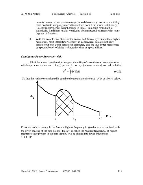
ATM 552 Notes: Time Series Analysis - Section 6a Page 115noise is present, a line spectrum may (should) have very poor reproducibilityfrom one finite sampling interval to another; even if the series is stationary(i.e., its true properties do not change in time). To obtain reproducible,statistically significant results we need to obtain spectral estimates with manydegrees of freedom.3. With the notable exceptions of the annual and diurnal cycles and their higherharmonics, most interesting “signals” in geophysical data are not trulyperiodic but only quasi-periodic in character, and are thus better representedby spectral bands of finite width, rather than by spectral lines.Continuous Power Spectrum: (k)All of the above considerations suggest the utility of a continuous power spectrumwhich represents the variance of y i (t) per unit frequency (or wavenumber) interval such thaty' 2 k*= ( k)dk (6.26)0So that the variance contributed is equal to the area under the curve (k), as shown below. kkk1 2k*kk* corresponds to one cycle per 2t, the highest frequency in y(t) that can be resolved withthe given spacing of the data points. This k* is called the Nyquist frequency. If higherfrequencies are present in the data set they will be aliased into lower frequencies.0 k k*Copyright 2005 Dennis L. Hartmann 1/25/05 5:04 PM 115