Perceptions and Expenditure Patterns - Social Policy Research ...

Living Standards after Retirement: Perceptions andExpenditure PatternsBruce Bradbury and Silvia MendoliaFinal Report from the Project: ‘Expenditure Costs’Social Policy Research Centre,May 2012SPRC Report 2/12

Social Policy Research Centre, UNSWResearch teamDr Bruce BradburySilvia MendoliaAuthorsDr Bruce BradburySilvia MendoliaContact for follow upBruce Bradbury, Social Policy Research Centre, University of New South Wales,Sydney NSW 2052, Ph: (02) 9385 7814, b.bradbury @unsw.edu.auNotesThe research reported in this paper was completed under FaHCSIA’s Social PolicyResearch Services Agreement (2005–2009) with the Social Policy Research Centre.The opinions, comments and/or analysis expressed in this document are those of theauthors and do not necessarily represent the views of the Minister for Families,Housing, Community Services and Indigenous Affairs or the Australian GovernmentDepartment of Families, Housing, Community Services and Indigenous Affairs(FaHCSIA), and cannot be taken in any way as expressions of Government policy.This paper uses confidentialised unit record file from the Household, Income andLabour Dynamics in Australia (HILDA) survey. The HILDA Project was initiated and isfunded by the Commonwealth Department of Families, Community Services andIndigenous Affairs and is managed by the Melbourne Institute of Applied Economicand Social Research (MIAESR). The findings and views reported in this paper,however, are those of the authors and should not be attributed to either FaHCSIA orthe MIAESR.Suggested CitationBradbury, B and Mendolia, S. (2012), ‘Living Standards after Retirement: Perceptionsand Expenditure Patterns’’, prepared for the Department of Families, Housing,Community Services and Indigenous Affairs under the Deed of Agreement for theProvision of Social Policy Research Services.Contentsiii

Summary ....................................................................................................................... 11 Introduction ......................................................................................................... 32 Background .......................................................................................................... 43 Expectations and perceptions ............................................................................. 63.1 Retirement expectations ........................................................................................... 63.2 Perceptions of living standards and financial hardship ............................................ 73.3 Interpretation .......................................................................................................... 144 Expenditures in retirement ............................................................................... 164.1 The impact of retirement on expenditure patterns ................................................. 164.2 Expenditure data .................................................................................................... 194.3 Descriptive patterns of expenditure ....................................................................... 204.4 The cost (savings) of retirement............................................................................. 245 Conclusions ........................................................................................................ 276 References .......................................................................................................... 287 Appendix ............................................................................................................ 30iv

SummaryHow much income do people need in retirement in order to maintain their pre-retirement standardof living? In answering this question, this report addresses two sets of issues.The first set concerns people’s expectations of retirement and their perceptions of their livingstandards after retirement. Do people who are not yet retired expect that they will be able tomaintain their living standards in retirement? Do retired people consider that they have actuallymaintained their standard of living? How do perceptions of financial hardship and financialsatisfaction and prosperity change as people age?The second set of questions addresses the actual expenditure patterns of retired people. Do thesepatterns suggest that the expenditure needs of retired people are less than those of people in thepre-retirement years?Data from the first six waves of the Household Income and Labour Dynamics in Australia survey(HILDA) (2001 to 2006) are used to investigate people’s expectations and perceptions (Section 3).About a third of people who have not yet retired believe that they will not have enough inretirement to maintain their standard of living. Among those who had already retired, about half feelthat their current income is less than they had expected, and only 13 per cent consider it to be morethan expected. However, when asked about their standard of living since retirement, the fractionsaying it had decreased was similar to the fraction saying it had increased. The disparity betweenthese two patterns could be due to reductions in expenditure needs, or it could be due to peoplechanging their minds about what constitutes an acceptable standard of living in the light of incomereductions.The HILDA survey also contained information on people’s perceptions of their prosperity and theirreported satisfaction with their financial situations. We find that the former does not change muchwith age, while the latter increases strongly as people age. Similarly, experience of financial hardshipdeclines steeply with age. This is despite the fact that income falls steeply across the retirementyears in Australia.On the face of it, these results suggest that people are content with their attained living standards inretirement. This contentment, however, could reflect preference adaption to a situation of lowerliving standards (possibly in conjunction with other factors such as reduced volatility of income).Section 4 of the report uses data from two ABS Household Expenditure Surveys (HES) (1998-99 and2003-04) to examine expenditure patterns in retired and non-retired households.There are changes in household expenditure patterns that are directly influenced by retirement.These include the reduction in the costs associated with working, price concessions associated withpension receipt, and increased health costs. Under plausible simplifying assumptions, expenditureon goods other than these directly affected goods can be used as an indicator of living standards.The data from the HES surveys suggest that decreases in working expenses are more than offset byincreases in health-related costs after retirement. If anything, the evidence suggests that afterhousingincome should increase after retirement to allow households to maintain the same level ofnon-retirement-related expenditure they had prior to retirement.1

There is thus a disjuncture between falling incomes, maintained or increased financialsatisfaction and greater expenditure needs in retirement – ‘a retirement satisfaction puzzle’.We speculate that the observed subjective satisfaction with living standards among theelderly primarily reflects an adaption to reduced actual living standards and possibly theinfluence of peer effects.However, it is possible that our conclusions are influenced by our decisions about thosegoods that are assumed to not be directly affected by retirement. A natural extension to thisresearch will be to test whether the conclusions are robust to alternative ways of definingsuch categories of goods.2

1 IntroductionWhat should be the income target for retirement income policy? Should it seek to maintain effectiveconsumption at the same level as pre-retirement? If so, how much do retired people need to spendin order to maintain their standard of living? Answers to these questions are crucial to retirementincome policy – but evidence is scant.Uncertainty in this area stems from two sources. First, it is not clear what the objective of retirementincomes policy should be. Should it seek to maintain living standards at pre-retirement levels, orshould policy accept that living standards will fall in retirement? Answers to this will depend uponsocial norms of behaviour and objectives which might change over time. Second, any suchframework objective then needs to be assessed in the light of evidence of actual patterns. In doingthis, we need to assess how living standards should be measured in this context, and whether theydo in fact fall after retirement.This report addresses two specific sets of questions. The first set, discussed in Section 3, concernsexpectations and perceptions of living standards. Do people who are not yet retired expect that theywill be able to maintain their living standard in retirement? Do retired people consider that theyhave actually maintained their standard of living? How do perceptions of financial hardship andfinancial satisfaction and prosperity change as people age? The second set of questions addressesthe observed expenditure patterns of retired people (Section 4). Do they suggest that theexpenditure needs of retired people are less than those of people in the pre-retirement years? If so,by how much are expenditure needs reduced (or increased)?The results of these two sets of investigations are contradictory. Income and expenditure declinewith age, but people are generally satisfied and less likely to report financial hardship. Afterretirement, some expenditure needs decrease (eg work expenses) while others increase (eg healthcare costs). The data from the HES surveys suggest that the latter effect dominates. This implies that,in order to maintain their pre-retirement level of expenditure on goods that are not affected byeither type of change, retired people would need to increase their total (after-housing) income andexpenditure in retirement.The report concludes with a discussion of possible limitations of the analysis and suggestions forfurther research.3

2 BackgroundThough there is substantial discussion of policies that might enable people to reach variousexpenditure targets in retirement, there is very little research seeking to define these targets. Somecommentators simply assume that consumption needs are constant with age (e.g. Yuh, Montaltoand Hanna, 1998); others apply simple ‘rules of thumb’.Vince FitzGerald reported on these different approaches to the 2002 Senate Select Committee onSuperannuation (SSCS, 2002). He reported a general tendency across the OECD for retirementincome systems to aim at disposable income replacement rates of around 70 to 80 per cent(comparing disposable incomes immediately before and after retirement). In its conclusions, theSenate committee concluded that there was a strong degree of consensus for average replacementlevels of expenditure of around 70-80 per cent. This ratio should be higher for those on low incomesand lower for those on high incomes, and any adequacy benchmark should focus on consumptionlevels in the first year of retirement.Though this ratio is numerically identical to the one proposed by FitzGerald, it refers to a differentconcept. FitzGerald was referring to ratios of disposable income rather than to ratios of expenditure.For the elderly, these are often different. Expenditure might be higher than income because theycan draw on savings, and consumption might be higher still because of the services provided byowner-occupied housing. In any event, the evidence basis for recommendations based on eitherapproach is very thin.There is, however, extensive research on the actual consumption behaviour of people in retirement.A key question here is the ‘retirement consumption puzzle’. 1 Economic life-cycle theory suggeststhat people should use borrowing and saving to smooth their consumption over time – particularlywith respect to anticipated events such as retirement. But there is strong evidence that expendituretends to fall after retirement.This is partly explained by reductions in work-related expenditures. However, most researchers alsoobserve reductions in food expenditures, which are more likely to be due to falls in living standards(though there could potentially be some reductions due to increased home production). Barrett andBrzozowski (2009) examined this issue using the grocery and food expenditure measures collected inthe Australian HILDA survey. They found a fall in grocery spending of around 7 per cent and a fall infood expenditure of 8-9 per cent associated with the transition to retirement – supporting theconclusions of the international literature that consumption falls with retirement. Measures ofreported financial hardship, however, do not show a clear pattern, possibly suggesting somehabituation to lower living standards.Four possible explanations could be advanced for this finding of falling consumption in retirement.It is an artefact of incorrect measurement of true consumption, e.g. not taking full accountof home production.Consumption is in fact lower in retirement – and people are surprised by this once theyreach retirement.1See the surveys by Hurst (2008) and Barrett and Brzozowski (2009).4

3 Expectations and perceptionsDo people expect that they will be able to maintain their living standard in retirement? Do retiredpeople consider that they have maintained their previous standard of living? How do perceptions offinancial hardship and financial satisfaction and prosperity change as people age? This sectionaddresses these questions using data from the Household Income and Labour Dynamics in Australiasurvey (HILDA). This is a large nationally representative panel survey of Australian households. Datafrom the first six waves of the survey (conducted from 2001 to 2006) are used here. (For moreinformation on the survey, see Watson, (ed) 2009).3.1 Retirement expectationsIn 2003, the HILDA survey asked respondents about their expectations and experiences of livingstandards after retirement. Table 1 summarises some of these responses. People who had not yetretired were asked whether they anticipated being able to maintain their standard of living afterretirement. A substantial fraction, just over one-third, reported that they did not expect to haveenough to maintain their current standard of living.Table 1 Living standards in retirement: expectations and experience(HILDA Wave 3, 2003)People aged 45 or more, who have not yet (completely) retiredDo you expect your retirement income to be more than enough, just enough or notenough to maintain your current standard of living?% (weighted)More than enough 9.2Just enough 56.7Not enough 34.0Total 100.0N (unweighted) 2,807People who have retired and are not workingWould you say (your standard of living) is better or worse since you retired?Much worse 5.8Worse 21.8The same 51.6Better 15.5Much better 5.3Total 100.0N (unweighted) 1,206Thinking about your current income [from all sources], is this more or less thanyou had expected it to be when you retired?Much less 24.4A little less 26.0About the same 36.4A little more 11.1Much more 2.2Total 100.0N (unweighted) 1,175Notes: Source, HILDA Wave 3 (Release 5.1). Cross-section weights used.6

People who had already retired were asked to compare their standard of living before andafter retirement. About half said it was the same. Of the remainder, 27 per cent reported aworse standard of living and 21 per cent a better standard of living. 4 They were also askedwhether their current income was what they anticipated before retirement. Around halfreported that it was less than expected.One possible interpretation of these results is that the very substantial drop in incomeassociated with retirement was unanticipated by the current retired generation, but that thenext generation about to retire now expects it. Though people are more likely to say that boththeir living standards and their incomes have deteriorated since retirement than to say theyhave improved, the difference is not large. This could be because there are offsetting costreductions associated with retirement, or it could be because people reduce their expectationsof ‘standard of living’ so as to require less expenditure.3.2 Perceptions of living standards and financial hardshipThe HILDA survey also regularly collects information on respondents’ evaluations of their financialsituations and reports of financial hardship. 5Respondents are asked in the interview part of the survey to score their satisfaction with differentaspects of their lives on a 0-10 scale (high scores indicating more satisfaction). One of these aspectsis satisfaction with financial situation. (Others include home, employment opportunities, how safethey feel, community, health and neighbourhood, and amount of free time). For the purpose of thispresent report, the variable, satisfaction with financial situation, is standardised with a mean of zeroand a standard deviation of one (for the population of people aged 45 and over).In the self-completion questionnaire part of the survey, respondents are asked a question abouttheir perceived prosperity. ‘Given your current needs and financial responsibilities, would you saythat you and your family are... Prosperous, very comfortable, reasonably comfortable, just gettingalong, poor, very poor?’ This is mapped onto a six-point scale (high scores recoded here to indicatemore prosperity) and standardised as for the satisfaction score.They are asked whether any of a number of events had occurred for them since the beginning of theyear because of a shortage of money:could not pay electricity, gas or telephone bills on timecould not pay the mortgage or rent on timepawned or sold somethingwent without mealswas unable to heat homeasked for financial help from friends or familyasked for help from welfare/community organisations45In addition, most people reported having more leisure and more reported being happier (not shown here).Similar information is collected in the ABS HES. The HILDA survey data is used here to take advantage ofthe repeated collection of this information over several waves.7

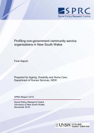
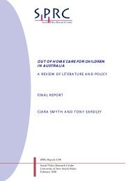
We begin by considering the first six waves of the HILDA survey as a pooled cross-section survey (ieignoring the panel structure of the data). To put the indicators of financial prosperity and hardship incontext, Figure 1 shows the average equivalent income of each age group. Though some of thepattern shown in the figure might reflect cohort effects, most of the pattern is likely to stem fromlifecycle changes in income. After a peak at age 50-59, average household income declines steadilywith age. Even taking into account the smaller household size in later years, equivalent income whenpeople are aged in their 70s is only around half the income they had in their 50s. This is not offset byincreases in wealth, since average wealth holdings also decline after retirement age. 6Figure 1Average household equivalent income by age$2006-07 pa50,00045,00040,0001 person household2 person householdAll (including larger households)35,00030,00025,00020,00015,00010,00045-49 50-54 55-59 60-64 65-69 70-74 75-79 80+AgeNotes: Source HILDA survey, waves 1 to 6. The table shows mean annual equivalent household disposableincome of individuals for the financial years 2000-01 to 2005-06, inflated to 2006-07$ using the CPI.The equivalence scale is the square root of the number of people in the household (for single people,equivalent income equals actual income).Figure 1 shows a consistent difference in average equivalent income between couples and singles,but this is an arbitrary feature of the square-root equivalence scale used to calculate equivalentincome. The square-root scale assumes that singles need around 71 per cent of the income ofcouples in order to reach the same living standard. The pension relativity was around 61 per centprior to 2009, and was increased to around 67 per cent as a result of the recommendations of theHarmer Review in 2009 (Harmer, 2009). 7Figure 2 puts these age-related patterns in the context of retirement. People are defined as retiredin this figure if they had previously worked for two weeks or more, were now not in the labour force(i.e. were neither employed nor unemployed) and did not intend to look for, or do, paid work in thefuture. For both sexes, retirement rates increase steadily from the late 40s. By age 60-64, 36 per67See ABS Cat No 6554.0 Household Wealth and Wealth Distribution, Australia, 2003-04, Table 20.See also Bradbury (2009) for further discussion of Age Pension relativities, and Bradbury and Gubhaju(2009) for further information on the incomes of the older population.8

cent of men and 57 per cent of women are retired under this definition. By age 65-69, thesepercentages have increased to 68 and 84 per cent respectively. Among the 70+ age group, some 9per cent of men say that they have not retired.Figure 2 Self-described retirement by age, 2007100%9080706050403020100WomenMen45-49 50-54 55-59 60-64 65-69 70+AgeNotesExcludes people who had never had paid work for two weeks or more and people whose retirementstatus could not be determined. Source, ABS 4102.0 Australian Social Trends, March 2009 (originalsource ABS cat. No. 6361.0).This definition of retirement is not the only one that is commonly used. 8 For many policy purposes,an explicit age-based criterion is more useful, as age defines eligibility for Age Pension. For thisreason, and also because unobserved selection effects could lead to correlations between subjectiveviews about future work plans and perceptions of financial hardship, age is used as the primaryindicator of retirement in most of the results that follow.Figure 3 shows the mean levels of financial satisfaction and prosperity by age (standardised asdescribed above). Perceived prosperity is roughly constant across age groups, but there is a strongtendency for satisfaction with financial situation to increase with age, despite the associated steadyfall in income.8For further discussion of the complexities of defining retirement and retirement expectations, see Cobb-Clark and Stillman (2009).9

Figure 3Deviationfrommean(std dev)0.60.50.40.30.20.10-0.1-0.2-0.3Average financial satisfaction and prosperity by ageSatisfaction with financial situationPerceived prosperity45-49 50-54 55-59 60-64 65-69 70-74 75-79 80+AgeNotes: Source HILDA survey, pooled cross-section data from waves 1 to 6. Both variables are standardised tomean of zero and variance of one.Figure 4 shows the proportion of the population aged 45 and over who reported different forms offinancial hardship. The measures generally decrease with age, 9 again, despite the decrease inincome. For the two measures describing not being able to pay bills on time, the rate among the 65-69 age group is slightly higher than that among the 60-64 age group, suggesting some problems inadjusting to new lower income levels. There is also an indication of these measures increasing in theoldest two age groups, particularly with respect to asking for help from welfare or communityorganisations. However, even though the question asks about this help in the context of a shortageof money, it is possible that people interpret it to mean asking for help because of disability or illnessrather than because of financial need per se.9The slope of the decrease is greater for those measures that have higher initial levels of hardship. However,in proportionate terms (e.g. when using a log vertical scale) the slopes are similar for all the measures(except where the ‘asking for help from welfare organizations’ measure turns up).10

Table 2 The association between financial satisfaction and prosperity with ageMen and womenCross-section OLSFixed effectsEffect size t Effect size tPerceived prosperityAge 55 minus age 45 0.13 2.8 0.09 1.6Age 65 minus age 55 0.01 0.5 0.10 1.7Age 75 minus age 65 -0.01 -0.7 0.08 1.3Age 85 minus age 75 0.06 1.6 0.04 0.5Financial satisfactionAge 55 minus age 45 0.13 3.3 0.15 2.9Age 65 minus age 55 0.17 9.4 0.23 5.3Age 75 minus age 65 0.20 9.1 0.19 4.2Age 85 minus age 75 0.22 7.1 0.05 0.8Women onlyCross-section OLSFixed effectsEffect size t Effect size tPerceived prosperityAge 55 minus age 45 0.10 2.1 0.15 2.4Age 65 minus age 55 -0.01 -0.3 0.11 1.9Age 75 minus age 65 -0.02 -1.0 0.08 1.1Age 85 minus age 75 0.04 0.9 0.04 0.4Financial satisfactionAge 55 minus age 45 0.13 2.8 0.07 0.9Age 65 minus age 55 0.19 8.5 0.17 2.6Age 75 minus age 65 0.21 7.8 0.13 1.7Age 85 minus age 75 0.19 6.2 -0.05 -0.6Notes: Calculated from the HILDA survey, waves 1 to 6. The dependent variables are financial satisfactionand perceived prosperity scores, normalised to have standard deviation of one. The parameter estimatesare thus effect sizes, showing the number of standard deviation units increase in the dependent variablewhen increasing age by 10 years. The left-hand panel shows a pooled OLS estimation, including acubic function of age and dummy variables for each survey wave. The right-hand panel shows a fixedeffects estimation, controlling for waves 3 to 6 (vs waves 1 or 2). The ‘t’ columns show the estimatedivided by the standard error, calculated using the cross-section replication weights provided in theHILDA survey (absolute values greater than 1.96 are significant at the 5% level).The top-left number in Table 2 shows that as people increase from age 45 to age 55, their expressedfinancial satisfaction increases by 0.13 standard deviations – a small, but statistically significant,increase. Subsequent decades see no increase, though there is a small (not significant) increase afterage 75. This mirrors the pattern shown in Figure 3, as does the steady increase in financialsatisfaction, shown in the second panel.These estimates also control for the survey wave in which the data was collected. These parameters(not shown) indicate that perceived prosperity and satisfaction increased significantly after thesecond wave, possibly due to changes in the survey methodology. The fixed effects estimates on theright-hand side of the figure also control for interview wave, but only by distinguishing betweenwaves 1 or 2 vs the remaining waves. It is not possible to control for each wave separately, as thechange in wave is strongly associated with the change in age.12

Table 3Association between financial hardship and ageIncrease inincidence (%)Could not pay electricity, gas or telephone bills on timeAge 55 minus age 45 -5.5 -3.6Age 65 minus age 55 -3.4 -5.3Age 75 minus age 65 -1.2 -2.4Age 85 minus age 75 0.4 0.6Asked for financial help from friends or familyAge 55 minus age 45 -4.8 -4.5Age 65 minus age 55 -2.8 -6.1Age 75 minus age 65 -1.8 -4.8Age 85 minus age 75 -0.8 -2.3Could not pay the mortgage or rent on timeAge 55 minus age 45 -3.2 -3.5Age 65 minus age 55 -1.8 -5.4Age 75 minus age 65 -0.3 -1.2Age 85 minus age 75 0.5 1.0Pawned or sold somethingAge 55 minus age 45 -4.0 -3.5Age 65 minus age 55 -0.8 -2.4Age 75 minus age 65 -1.3 -3.2Age 85 minus age 75 -0.7 -4.0Asked for help from welfare/community organisationAge 55 minus age 45 -1.7 -2.2Age 65 minus age 55 -0.7 -2.5Age 75 minus age 65 0.0 -0.1Age 85 minus age 75 0.7 1.1Went without mealsAge 55 minus age 45 -1.1 -1.3Age 65 minus age 55 -1.1 -3.3Age 75 minus age 65 -0.8 -3.5Age 85 minus age 75 -0.3 -1.9Was unable to heat homeAge 55 minus age 45 -0.2 -0.3Age 65 minus age 55 -0.5 -1.6Age 75 minus age 65 -0.1 -0.4Age 85 minus age 75 -0.1 -0.2Notes: Calculated from the HILDA survey, waves 1 to 6. Estimated via a logistic regression across the pooledcross-section. The regression includes a quartic function of age, sex and flags for each wave of thesurvey. The estimates show the predicted increase in incidence when increasing age by 10 years asindicated. The ‘t’ column shows the estimate divided by the standard error calculated using the crosssectionreplication weights provided in the HILDA survey (absolute values greater than 1.96 aresignificant at the 5% level).tThe fixed-effects regression model shows the impact of changes in age on changes in expressedsatisfaction or prosperity. This is equivalent to a regression that includes a dummy variable for each13

person. If, for example, the patterns shown in the cross-section regression were due to differentcohorts having different expectations, 11 this would not appear in the fixed-effects regression.From the data shown here, it is not obvious which estimation approach is more valid, as the fixedeffects estimates cannot fully control for changes between the survey waves (e.g. changes due tomacro economic conditions). However, the results from both approaches are broadly the same. Thefixed effects estimates show a somewhat greater increase in perceived prosperity than the OLSestimates, but a similar increase in financial satisfaction. Both approaches show that financialsatisfaction and prosperity either increase or stay constant as people age.The picture for women shown in the bottom half of the table is similar to the pattern for men andwomen combined. The only difference is that the fixed effects estimates for financial satisfactiontend to increase with age at a slower rate than for the population in general.Table 3 shows the cross-sectional relationship between the different financial hardship measuresand age. This table mirrors the relationships shown in Figure 4. With a few minor exceptions, all thehardship measures decrease with age, but at a decreasing rate. Though Figure 4 shows somemeasures of hardship increasing with age, Table 3 shows that none of the increases is statisticallysignificant.3.3 InterpretationAfter peaking for people in their mid-50s, the average income of Australians declines steeply as theyage. At the same time,their perceived prosperity stays roughly constant;their satisfaction with their financial situation strongly increases; andtheir experience of financial hardship (such as not being able to pay bills, or having to ask forfinancial help) declines steadily.How should we interpret this apparently paradoxical relationship between income and perceptions?One interpretation is that needs decline faster than income (and wealth). This would imply that thecurrent system of income support for the elderly was more than sufficient for them to maintain theirsatisfaction with their financial situation and to avoid hardship. In turn, this suggests that attemptsto expand the provision of income support for the aged via the expansion of superannuation beyondthe current model were not needed, and that the Age Pension was already quite effective inameliorating financial stress.However, the widespread political support for superannuation and adequate Age Pensions mustsurely weigh against this explanation. It is also inconsistent with cross-national evidence showingthat the fall in income after retirement is particularly steep in Australia – even though this is offset tosome extent by a high level of home ownership (Bradbury, 2008).An alternative explanation for the paradox is that these responses reflect factors other than just thestandard of living of the respondents. In particular, expectations and financial management are likelyto be important. For example, people may lower their expectations as they age, and establish more11Or different mortality rates among people with different satisfaction levels.14

stable patterns of income and consumption. A greater stability of finances in old age, in particular,might reduce the prevalence of problems of not being able to pay bills or needing to ask for financialhelp. In addition, we cannot assume that these expectations will also be maintained in the future –when cohorts with experience of higher consumption levels reach retirement.It is thus not clear whether these expressions of financial prosperity and hardship should be taken atface value. The next section draws upon the quite different evidence of household expenditurepatterns to examine these issues.15

4 Expenditures in retirement4.1 The impact of retirement on expenditure patternsDo people need to spend less (or more) to maintain the same standard of living in retirement? Formost people, both income and expenditure fall after retirement. The results of the previous sectionsuggest that satisfaction with financial situation increases after retirement while the experience offinancial hardship decreases. If these are used as the standard of living indicator, they suggest thatpeople need substantially less in retirement. But possibly this represents changes in expectationsassociated with retirement. What happens if we focus more directly on the consumption patterns ofthe retired? Does this also indicate that less is needed?As noted in the introduction, previous research suggests that consumption expenditures do fall inretirement. Why would people choose to have a lower standard of living at one particular stage oftheir life? This has been described as the ‘retirement consumption puzzle’. One answer to thisquestion relates to variations in needs across the life cycle. There are several reasons whyexpenditures might be expected to change after retirement, even when people maintain the sameliving standard:Reductions in work-related costs. These include reductions in transport costs, work-relatedclothing and meals out (e.g. lunch purchases).Increases in health service consumption because of increased age. Even though this is afunction of age rather than retirement per se, the strong association between the twomeans that we should probably consider this as a characteristic of aging and retirement.Some of these increases in consumption are offset by the lower prices associated withpension or seniors’ concessions. Although some of these concessions are available to peopleprior to retirement, and not all retired people receive pensioner concessions, the price ofmany items is lower for the average retired person.At the same time, retirement is associated with a very different pattern of time allocation.More time for home production will generally (but not necessarily) result in reducedexpenditure, e.g. a switch from the purchase of prepared food items to food ingredients.Similarly, there may be an increase in some leisure activities, which might increaseexpenditure on associated items.Life-cycle patterns in housing financing. Most Australian households follow a typical lifecyclepattern of housing finance which means that the consumption of housing services can differsignificantly from their housing expenditures. For a household that stays in the samedwelling over the retirement transition, their consumption of housing services will beroughly constant. However, their typical expenditure on both mortgage principal andinterest payments will steadily fall.In the appendix, a table describing the over 600 different commodity categories available in the HESsurveys is presented, with our estimation of whether expenditure on the commodity is influenced byany of the first four retirement-specific factors described above. (Rents and mortgage repaymentsare excluded separately). These assumptions are summarised in Table 4.Among couple households with husband over 50, around 17 per cent of current expenditure is spenton commodities that are at least partly work-related. These include transport, eating out and16

clothing. Around 7 per cent is spent on health-related expenditures and 12 per cent on commoditieswhere there are significant price reductions for pensioners (who comprise the majority of the retiredpopulation). Most health commodities appear in both these groups. We consider that there are asmaller volume of expenditures affected by home production changes (4%, mainly homemaintenance, gardening, cooking). Around 7 per cent of expenditures are on commodities whereexpenditure might be expected to increase.Of more relevance for the final estimates of costs are the commodity categories where we do notexpect to find a direct impact of retirement on expenditure needs. These are summarised in Table 5.The main commodity areas where we think it reasonable to assume that costs are not directlyaffected by retirement are: food (except eating out and snack food); household furniture, linen andappliances; communication charges; and overseas holidays.In compiling these lists we have sought to be reasonably restrictive in defining what is specificallyrelated to retirement. For example, in the area of holiday travel, we have included caravans anddomestic travel costs as retirement-related as these are part of the (Australian) stero-typical patternof becoming a ‘grey nomad’. Overseas travel, however, has not been considered retirement specific,as this is common at all ages. One could think of factors both encouraging and discouraging overseastravel after retirement. On the one hand retired people have more time for travel, while on theother, poorer health and higher health insurance costs would discourage it.Note that we include many household durables (furniture, appliances, electronic goods) in ourcategory of goods that are not directly affected by retirement. If people upgrade these goods in theretirement years with the intention of consuming them in the post-retirement years, this might notbe appropriate. However, these patterns of purchases might equally be considered a response to thedifferent income levels in pre and post-retirement, and so our approach would be appropriate.To put this another way, our estimate of the expenditure needs in retirement will thus be anestimate of the income needed in order to maintain constant expenditures on these classes ofgoods. If incomes don’t, in fact, follow this pattern then shifting expenditures to earlier periods isone way of compensating for this.17

Table 4 Expenditure categories directly influenced by retirementReductions in work-related costs (17%)Large effect (10%) pre-prepared meals, non-alcoholic beverages, meals out; men’s suits, trousers, shirts; women’s trousers, skirts, dresses, suits, shirts and blouses; motor vehicle fuel, oil, tyres, servicing, tolls; public transport; union dues.Smaller effect (7%) women’s hosiery; ties/gloves/handkerchiefs; motor vehicle purchase, registration, insurance, repairs.Increases in health service consumption (7%)Large effect (7%) home help; hospital, medical and dental insurance (not ambulance); doctors’ and dentists’ fees; medicines, ointments, dressings, nursing charges; taxi fares, travel insurance.Price reductions (12%)Large effect (7%) electricity and gas; doctors’ fees, opticians’ fees, prescription medicines, therapeutic appliances; hospital and nursing home charges; public transport, holiday rail fares; health and fitness studio fees, museum/park entrance fees, culture/recreation courses.Smaller effect (5%) non-prescription medicines, entertainment fees, holiday bus fares; hair, personal care services.Home production (4%) (expenditure reductions unless noted)Large effect (3%) paint and house-painting contractors, misc. maintenance contractors and supplies; cardigans and pullovers; repairs and cleaning of clothes; clothing materials and gardening tools (increase); gardening, housekeeping and cleaning services.Smaller effect (1%) cakes, etc., cake mixes, biscuits; cooking utensils and other tools (increase); plants (increase); animal minding charges.Leisure expenditure increase (7%)Large effect (3%) purchase and registration of caravan or trailer, domestic holiday expenses; golf equipment and fees; day trips, culture and recreation lessons; pay TV.Smaller effect (4%) petrol; fishing equipment, health studio charges; entertainment.Notes: See Appendix table for more details. Numbers in brackets are budget shares in 2003-04 (over-50population as described below). For home production, this is the budget share of commodities withexpected expenditure reductions. Some commodities appear in more than one category. Rents andmortgage repayments are not included.18

Table 5Expenditure categories not directly influenced by retirement house and contents insurance, most repairs and maintenance, loans, body corporate payments second dwelling costs most foods except eating out, non-alcoholic drinks, cakes and biscuits clothing except as specified in work-related in Table 4 furniture, linen, appliances, utensils, household supplies electronic equipment and communication charges books, gambling, sports equipment (other than golf) non-prescribed pain relievers, sunscreens airfares, holiday vehicle hire, overseas holidays pets personal care (except hair care) watches, clocks and other personal expenditures, gifts4.2 Expenditure dataData from the two most recent ABS Household Expenditure Surveys (1998-99 and 2003-04) are usedto examine household expenditure patterns within these different categories. In order to restrict theanalysis to reasonably homogenous population groups, and to avoid complications associated withchanging household composition and different wealth levels, attention is restricted to marriedcouple, home-owning households aged 50 and over. More specifically, households are included ifthey satisfy the following conditions:they comprise a married or de facto couple onlythe husband is aged 50 or olderthe couple own their own home (including those with mortgages) the bottom and top 3 per cent of households ranked by after-housing income are excluded. 12This population is separated into the retired and ‘non-retired’ using two different criteria:Not in labour force: Neither partner is in the labour forceHusband 65+: The male partner is aged 65 or moreAs noted in the previous section, these are not the only way to define the status of ‘retired’. Thesecriteria are used here as they present a simple and unambiguous categorisation of households. Table6 shows the population size and overlap between the two definitions criteria in the two years.Slightly more households are defined as retired under the labour force definition in both years.However, there are a significant number of households in both non-overlapping cells. In 2003-04,around 17 per cent of couples where the husband was 65 or more had at least one of the couple inthe labour force, and around 21 per cent of couples who were not in the labour force had a husbandaged under 65 (the overlap is somewhat smaller in 1998-99).12Saunders and Bradbury (2006) provide evidence suggesting that income might not be accurately measuredamong the bottom 3 per cent of households (ranked by disposable income).19

Table 6 Sample size by retirement status, 1998-99 and 2003-04Husband 65+Either partner in labour forceNo Yes Total1998-99Yes 358 63 421No 111 451 562Total 469 514 9832003-04Yes 461 102 563No 129 483 612Total 590 585 1175Notes: Population is home-owner couples with husband aged 50+ (top and bottom 3% of after-housing incomeexcluded).Table 7 shows the average expenditure patterns and budget shares for the different categoriesof expenditure listed in Table 4 and Table 5, for retired households under both definitions.Note that expenditure on housing finance is treated differently to the other goods whencalculating budget shares. The objective is to end up with estimates of the extent to whichafter-housing household income (or non-housing expenditure) needs to increase or decreaseso as to maintain living standards constant in retirement. Housing finance expenditure is bothvery variable between households but also a category of expenditure where individualhouseholds are able to make reasonable forecasts of future expenditures. Hence, it isappropriate to treat this as a separate item to be considered after non-housing needs arecalculated.After-housing income is defined as the gross income of the household minus income tax andmortgage payments (for the dwelling in which the couple live), both principal and interest.Total non-housing expenditure is defined as total current expenditure on goods and services,minus expenditure on home loan interest repayments (for this dwelling). Note that this ismore precisely defined as ‘total expenditure minus housing finance’, as other current housingexpenditures such as maintenance and land taxes are not deducted, and mortgage principalrepayments are already excluded because they are not included as a current expenditure. Nonhousingsaving (which might be negative) is defined as after-housing income minus totalnon-housing expenditure.4.3 Descriptive patterns of expenditureTable 7 shows the mean expenditures and budget shares of the categories of goods described abovefor 2003-04. Table 8 has the corresponding information for 1998-99. Goods are characterisedaccording to features that would make the goods specifically dependent upon retirement.20

Table 7 Mean expenditures and budget shares, 2003-04NoHusband 65+YesNot in labour forceNo /Yes No YesMean expenditures ($/week)Non-retirement expenditures 454.6 318.1 1.4 471.4 314.4 1.5 382.5Work related expenditures (only) 169.1 105.6 1.6 175.3 105.1 1.7 135.6Both work and leisure related changes 30.5 21.8 1.4 32.5 20.8 1.6 25.9Both work related and price reductions 2.8 1.1 2.6 3.1 1.0 3.2 1.9Work total 202.4 128.4 1.6 210.9 126.9 1.7 163.3Home production (only) 41.1 31.5 1.3 41.8 31.6 1.3 36.0Health related expenditures (only) 34.5 27.6 1.3 37.9 25.5 1.5 30.9Both health and price changes 24.3 21.3 1.1 24.8 21.2 1.2 22.7Health total 58.9 48.9 1.2 62.7 46.7 1.3 53.6Leisure related expenditures (only) 28.0 28.7 1.0 31.9 25.7 1.2 28.4Both leisure and price changes 7.1 4.0 1.8 8.0 3.5 2.3 5.4Leisure total 35.0 32.7 1.1 39.9 29.1 1.4 33.8Price reductions (only) 60.6 50.5 1.2 63.4 49.1 1.3 55.3Total non-housing expenditure 852.7 610.1 1.4 890.1 597.8 1.5 724.5Non-housing savings 44.0 10.5 4.2 116.6 -42.8 -2.7 26.3Total after-housing income 896.6 620.6 1.4 1006.7 555.0 1.8 750.8Total housing financing 48.7 2.6 19.1 47.5 6.6 7.2 24.3Expenditures as % of non-housing expenditure(calculated from top panel)No Change 53.3 52.1 1.02 53.0 52.6 1.01 52.8Work 23.7 21.0 1.13 23.7 21.2 1.12 22.5Home 4.8 5.2 0.94 4.7 5.3 0.89 5.0Health 6.9 8.0 0.86 7.0 7.8 0.90 7.4Leisure 4.1 5.4 0.77 4.5 4.9 0.92 4.7Price 7.1 8.3 0.86 7.1 8.2 0.87 7.6Total 100.0 100.0 1.00 100.0 100.0 1.00 100.0Expenditures as % of after-housing income(calculated from top panel)Non-retirement expenditures 50.7 51.3 0.99 46.8 56.7 0.83 50.9Work 22.6 20.7 1.09 21.0 22.9 0.92 21.8Home 4.6 5.1 0.90 4.2 5.7 0.73 4.8Health 6.6 7.9 0.83 6.2 8.4 0.74 7.1Leisure 3.9 5.3 0.74 4.0 5.3 0.76 4.5Price 6.8 8.1 0.83 6.3 8.8 0.71 7.4Savings 4.9 1.7 2.90 11.6 -7.7 -1.50 3.5Total 100.0 100.0 1.00 100.0 100.0 1.00 100.0Notes: Population is home-owner couples with husband aged 50+ (top and bottom 3% of after-housing incomeexcluded). Expenditure categories defined on the basis of any likely retirement effect. Source: ABSHES Survey, 2003-04.No /YesAll21

Table 8 Mean expenditures and budget shares, 1998-99NoHusband 65+YesNot in labour forceNo /Yes No YesMean expenditures ($/week)Non-retirement expenditures 439.7 310.6 1.4 456.4 310.2 1.5 366.3Work related expenditures (only) 145.0 111.1 1.3 156.0 106.9 1.5 125.7Both work and leisure related changes 26.3 20.2 1.3 28.0 19.7 1.4 22.8Both work related and price reductions 2.5 1.4 1.8 2.9 1.2 2.5 1.8Work total 173.7 132.7 1.3 186.8 127.7 1.5 150.4Home production (only) 34.8 31.8 1.1 36.6 30.9 1.2 33.1Health related expenditures (only) 29.1 24.9 1.2 33.9 22.3 1.5 26.7Both health and price changes 17.5 17.2 1.0 20.0 15.7 1.3 17.3Health total 46.6 42.1 1.1 53.9 37.9 1.4 44.0Leisure related expenditures (only) 18.6 20.6 0.9 16.5 21.7 0.8 19.7Both leisure and price changes 3.7 4.3 0.9 3.9 4.1 1.0 4.0Leisure total 22.3 24.9 0.9 20.5 25.8 0.8 23.8Price reductions (only) 56.3 47.1 1.2 59.0 46.1 1.3 51.1Total non-housing expenditure 773.3 589.3 1.3 813.2 578.7 1.4 668.6Non-housing savings -16.1 -61.7 0.3 31.1 -87.5 -0.4 -42.0Total after-housing income 757.2 527.6 1.4 844.3 491.2 1.7 626.6Total housing financing 34.4 3.7 9.3 38.5 3.5 10.9 17.0Expenditures as % of non-housing expenditure(calculated from top panel)No Change 56.9 52.7 1.08 56.1 53.6 1.05 54.8Work 22.5 22.5 1.00 23.0 22.1 1.04 22.5Home 4.5 5.4 0.83 4.5 5.3 0.84 5.0Health 6.0 7.2 0.84 6.6 6.6 1.01 6.6Leisure 2.9 4.2 0.68 2.5 4.5 0.56 3.6Price 7.3 8.0 0.91 7.3 8.0 0.91 7.6Total 100.0 100.0 1.00 100.0 100.0 1.00 100.0Expenditures as % of after-housing income(calculated from top panel)Non-retirement expenditures 58.1 58.9 0.99 54.1 63.1 0.86 58.4Work 22.9 25.2 0.91 22.1 26.0 0.85 24.0Home 4.6 6.0 0.76 4.3 6.3 0.69 5.3Health 6.1 8.0 0.77 6.4 7.7 0.83 7.0Leisure 2.9 4.7 0.62 2.4 5.3 0.46 3.8Price 7.4 8.9 0.83 7.0 9.4 0.74 8.1Savings -2.1 -11.7 0.18 3.7 -17.8 -0.21 -6.7Total 100.0 100.0 1.00 100.0 100.0 1.00 100.0Notes: Population is home-owner couples with husband aged 50+ (top and bottom 3% of after-housing incomeexcluded). Expenditure categories defined on the basis of any likely retirement effect. Source: ABSHES Survey, 1998-99. Estimates inflated to $2003-04 using CPI.There are some commodities which appear in more than one of the retirement-specific categories.The top panel of each table shows the mean expenditures for all the combinations that occur in thedata (and the ratios of the means for retired and not retired – the ‘No/Yes’ columns). The mainNo /YesAll22

mainly comprise utility charges and the like which increase in budget share as total expendituredecreases.The income share patterns, however, differ substantially between the two retirement definitions.This is because labour force participation has a larger impact on income than does being over 64.The impact on expenditures is relatively small, and so those couples not in the labour force arespending about 8 per cent more than their income in 2003-04 (18% in 1998-99). This, in turn, meansthat the income budget share of all commodity groups is higher among those couples not in thelabour force (other than savings, which is negative).4.4 The cost (savings) of retirementChanges in expenditure on retirement-specific goods do not necessarily reflect changes in livingstandards. Work-related expenditure is not part of household consumption, additional expenditureon health does not imply higher living standards if it is because of greater ill-health, and pricereductions might reduce expenditure without changing the quantity of goods consumed.However, expenditures on the non-retirement goods are not directly biased by such effects. The factthat these expenditures are much lower for the retired than for the non-retired thus providessupport for the findings of Barrett and Brzozowski (2009), based on data from HILDA, that averageexpenditure levels fall after retirement in Australia (the retirement-consumption puzzle). It must beremembered, however, that the data here is not longitudinal and compares different people whoare either retired or not retired. Part of the drop in expenditure shown here could thus be becauseyounger cohorts are richer. 13Price effects might also contaminate the relationship. More specifically, to use non-retirementexpenditure as an indicator of living standards requires the assumption that households havewelfare functions that are ‘separable’ between retirement and non-retirement goods and that thereare no important price effects that shift consumption between these two categories. Thisassumption implies that, for a given set of market prices, the amount spent upon ‘non-retirement’expenditures is influenced only by the household’s real standard of living. Price changes specific toretirement are assumed not to influence this allocation.However, many goods become cheaper for the average retired person because of pensioner andseniors’ concessions. If this led retired people to switch their expenditure towards these cheapergoods, then it would also lead to a reduction in expenditure on the ‘non-retirement’ goods, eventhough the household was no worse off. In this case, it would be wrong to conclude that the reducedexpenditure on these goods implied that they were worse off. Again, however, we would expectsuch effects to be small.On the above assumption about the separability of retirement and non-retirement goods, theinformation presented in Table 7 can be used to address the question of how much more (or less)people need in retirement to maintain their pre-retirement standard of consumption. If the amountthat people spend on ‘non-retirement’ goods is used as an indicator of their overall standard ofliving, then the relative need issue can be addressed by considering the question:13Even though Barrett and Brzozowski (2009) use panel data, the same caveat applies to their work (whichuses a random effects panel estimation approach).24

How high would the non-housing expenditure (or after-housing income) need to be in order forthe average retired person to spend as much on non-retirement goods as the average nonretiredperson?Both after-housing income and non-housing expenditure are considered, because it is not obviouswhich is the most appropriate policy objective. Income is appropriate because it is most closelyrelated to policy instruments such as pensions. However, it ignores the ability of people to drawdown on their wealth to finance their consumption. Expenditure that includes this draw-down is abetter indicator of the consumption level of the elderly.This approach is analogous to the Rothbarth (1943) method used to estimate the costs of children. 14That method uses expenditure on goods that are not consumed by children as an indicator of theliving standard of the adults in the household (both when they do and when they don’t havechildren). Here, the goods that are used are those that are not directly affected by retirement. Thekey assumptions of the Rothbarth approach (and hence this approach) are that preferences for adultconsumption (in this case, non-retirement consumption) are stable across the life cycle, that ‘adultgoods’ (in this case non-retirement goods) are indeed that, and that there are no distorting priceeffects (such as changes in consumption due to concessions).If we also assume that expenditure on non-retirement goods is always a constant proportion ofincome (or of total expenditure), this question can be answered from the data presented in Table 7.Let be expenditure on non-retirement goods and be income (or total expenditure) forhousehold t. For non-retired households, let and for retired households, ,where the parameters are the budget shares for the non-retirement goods shown in Table 7.Denote the average expenditure on non-retirement goods for the non-retired person asand for the retired person as . Equating these yields . So consumption ofnon-retirement goods will be equal whenThat is, the ratio of budget shares shown in bold in Table 7 shows the relative after-housingincome (or total non-housing expenditure) required in retirement to maintain consumption ofthat good.These ratios based on budget shares are in fact very close to one. This means that the averageretired couple needs to have the same total household expenditure as the average non-retiredcouple in order to maintain the same level of non-retirement expenditure. Reductions inexpenditure associated with reduced work-related costs are offset by increases due to changedhealth and leisure expenditure.The conclusions based on income shares using labour force status to define retirement are,however, somewhat different. Because couples out of the labour force are drawing upon theirsavings, they need only 83 per cent of the after-housing income of couples still in the labourforce.14See Deaton Muellbauer (1986) for more discussion of the Rothbarth approach.25

However, these conclusions derived from Table 7 depend upon the assumption thatexpenditures on the non-retirement goods are a constant fraction of total expenditure orincome (within each retirement category). In fact this is not the case. Non-retirement goodstend to be necessities, with lower-income households spending a much larger proportion oftheir budget on these goods. This lower income-elasticity (around 0.5), together with thelower average income of the retired, means that they may need to have a substantially largerincrease in total income in order to reach the same level of expenditure they had prior toretirement. To make this point another way, part of the reason why retired households haverelatively high budget shares for the non-retirement goods in the tables above is because theyhave a lower average living standard. The question we wish to answer here, however, is howmuch they would need in order to attain the same living standard as non-retired households.To estimate this, it is necessary to take account of the changing budget share of nonretirementgoods across the income distribution. This is done by estimating a quadraticrelationship between the logarithm of expenditure on non-retirement goods and the logarithmof after-housing income (or non-housing expenditure). 15 (1)Where if the household is classed as retired, 0 otherwise, and is an independentrandom error term of mean zero. Then expected expenditure on the non-retirement goods forretired and non-retired households will be equal whenwhere is the income level for a non-retired household and the income for the retiredhousehold. For a specified value of this equation is a quadratic in with solutionsgiven byThe ratio of the retirement to non-retirement income is thus given byEquation (1) is estimated using the two definitions of retirement and using either income ortotal expenditure on the RHS of the equation. After estimating the regression parameters, E iscalculated for values of at $480/week, $770/week and $1,080/week. These correspondapproximately to the 25 th , median and 75 th percentiles of income for couples where thehusband was under 65 in 2003-04. In general, the above equation implies up to two solutionsfor E – though one of these always implies a value for outside the bounds of our data,which we ignore.15The log form is used so as to reduce heteroscedascity. The constant budget share case can be estimated byfixing and . This yields estimates which imply results very similar to those implied byTable 7 and Table 8.26

The results of this regression are shown in Table 9. This table shows the relative afterhousingincome (or non-housing total expenditure) required by a retired couple in order forthem to have the same expenditure on non-retirement goods as a non-retired couple. Morespecifically, consider the top-left estimate of 1.36. This implies that, if a couple with at leastone member in the labour force has an after-housing income of $480 per week, then a couplewith no members in the labour force requires an after-housing income 36 per cent higher inorder for them to spend the same amount on non-retirement goods.Table 9Estimates of the relative needs of retired couplesAfter-housing income or expenditure level of non-retired couples$480/week $770/week $1,080/weekRetirement definition Estimate StandarderrorEstimate StandarderrorEstimate StandarderrorIncomeNot in the labour force 1998-99 1.36 0.13 1.11 0.11 1.00 0.122003-04 1.54 0.17 1.24 0.12 1.08 0.11Husband 65 + 1998-99 1.45 0.12 1.34 0.24 1.36 0.512003-04 1.57 0.15 1.35 0.13 1.22 1.22ExpenditureNot in the labour force 1998-99 1.04 0.04 1.08 0.06 1.14 0.082003-04 0.97 0.02 1.01 0.03 1.11 0.08Husband 65 + 1998-99 1.12 0.04 1.15 0.06 1.16 0.072003-04 1.02 0.03 1.05 0.03 1.09 0.06Notes: Source, ABS HES surveys, 1998-99 and 2003-04. Weighted data. Standard errors calculated using theABS replication weights and jacknife method.Particularly at the lower end of the income scale, all the ratios for both survey years and bothretirement definitions are well above one, 16 implying that retired couples need higher afterhousingincomes than non-retired couples. The ratios are generally higher in 2003-04 than1998-99, but these differences are not statistically significant. The ratios decline steeply asincome increases when using the labour force definition of retirement, but decline only asmall amount when using the age-based definition.The estimates in the second panel of the table, based on expenditure, are not as large, butalmost all are above one. These estimates show how much total non-housing expenditureretired households need in order to reach the same level of non-retirement spending. We areless confident of these estimates in the second panel, as they might be biased by theendogeneity of total expenditure. That is, any transitory shocks to non-retirement expenditurewill also be included in total expenditure. This will tend to increase the apparent relationshipbetween non-retirement expenditure and total expenditure, but it is not clear in whichdirection it will bias the relativity estimate. In future work, we will explore the use ofinstrumental variable approaches to control for this.5 ConclusionsThere is strong evidence that income and expenditure fall with the transition to retirement.This report’s conclusions on how households cope with this, however, are mixed.16And statistically significant. Approximate 95% confidence intervals can be estimated as2 standard errors.27

On the one hand, the results of the previous section suggest that, in order to be able tomaintain their level of commodity consumption, couples who retire need to increase (or atleast maintain) their previous level of income (after deducting housing costs). In fact,however, they decrease their income and expenditure. This apparent decrease in consumptionhas been described as the ‘retirement consumption puzzle’.The fact that households do not in fact maintain their income and expenditure suggests thatthey should be dissatisfied with their financial situation and more likely to report financialhardship. For the most part, however, this is not the case. Financial satisfaction increases andexperience of financial hardship decreases – though many retirees do say that their income inretirement is less than they expected it to be. We might call this result the ‘retirementsatisfaction puzzle’.Explanations for this disjuncture stem from the interpretation of either the satisfaction orconsumption measures. On the one hand, expectations might be low because peopleacclimatise to low living standards. This could be due to either cohort experience or becausepeople base their expectations on the experience of other people in similar situations (i.e.other retirees). Similarly, the older population might have less income volatility and hencefewer financial stress events, and yet still have a relatively low standard of living.On the other hand, writers such as Barrett and Brzozowski (2009) argue that the fall inexpenditure pattern after retirement is offset by other factors – such as reduced work-relatedexpenditure and increases in home production.Our evidence on expenditure patterns does not support this conclusion. We focus onexpenditures which we judge to be not directly affected by retirement in this fashion and findthat they too fall after retirement – implying a fall in real living standards. Another empiricaldifference is that Barrett and Brzozowski (2009) focus on the impact of retirement whileholding age constant, while we focus on the combined impact of these two factors. We arguethat the latter is the more relevant comparison for policies associated with consumptionmaintenance in retirement.Nonetheless, it might be the case that our definition of ‘non-retirement’ goods is open toquestion, with some goods that we include under this rubric being, in fact, directly tied upwith retirement patterns. For example, we include most foods as non-retirement goods, onlyexcluding those that clearly have a large home production element. The natural next stage forthis research, therefore, will be to disaggregate the non-retirement goods and to formally testwhether the different sub-categories of goods point to the same patterns of relative needs inretirement. 176 ReferencesBarrett, Garry and Matthew Brzozowski (2009), ‘The retirement – consumption puzzledownunder’ unpublished paper, June 2009.17The framework used in the cost of children literature can be used to undertake formal tests of thesehypotheses. See Deaton, Ruiz-Castillo and Thomas (1989).28

Bradbury, Bruce (1997), 'The living standards of the low income self-employed', TheAustralian Economic Review, 30 (4), 374-389.’Bradbury, Bruce (2008), ‘Asset rich, but income poor: Australian housing wealth andretirement in international context’ Final report of the project, Wealth holding patternsof Australia’s elderly. Report prepared for the Department of Families, Housing,Community Services and Indigenous AffairsBradbury, Bruce (2009), ‘The relative needs of single and couple age pensioners’, Finalreport from the project: Relative needs across the Age Pension population. Report toFaHCSIA, March 2009.Bradbury, Bruce and Bina Gubhaju (2009), ‘Housing costs and living standards among theelderly’, Draft final report for the project: Housing costs and living standards. Reportto FaHCSIA, July 2009.Cobb-Clark, Deborah A and Steven Stillman (2009), ‘The retirement expectations of middleagedAustralians’, The Economic Record, 85(269), June:146-163.Deaton, Angus, S. and John Muellbauer (1986), ‘On measuring child costs: with applicationsto poor countries’, Journal of Political Economy, 94(4), August, 720-44.Deaton, Angus, S; Javier Ruiz-Castillo and Duncan Thomas (1989), ‘The influence ofhousehold composition on household expenditure patterns: Theory and Spanishevidence’, Journal of Political Economy, 97(1):179-200.Denton, Frank T, Dean C Mountain and Byron G Spencer (2006), ‘Age, Retirement, andExpenditure Patterns: An Econometric Study of Older Households’, AtlanticEconomic Journal, 2006 (34), 421-434.Harmer, Jeff (2009), Pension Review Report, Commonwealth of Australia.Hurst, Erik (2008), ‘The retirement of a consumption puzzle’, NBER Working Paper No.13789.Rothbarth, E. (1943), ‘Note on a Method of Determining Equivalent Income for Families ofDifferent Composition’ Appendix IV in War-Time Pattern of Saving and Expenditureby Charles Madge, University Press, Cambridge.Saunders, Peter and Bruce Bradbury (2006), ‘Monitoring trends in poverty and incomedistribution: Data, methodology and measurement’, The Economic Record,82(258):341-364.Saunders, Peter, Jenny Chalmers, Marilyn McHugh, Colette Murray, Michael Bittman andBruce Bradbury (1998), Development of indicative budget standards for Australia,Research Paper No. 74, Department of Social Security.Saunders, Peter, Roger Patulny and Adeline Lee (2005), ‘Benchmarking the living standardsof older Australians using budget standards’, Australasian Journal on Ageing, 24 (3),September, 146-152.SSCS (Senate Select Committee on Superannuation) (2002), Superannuation and standardsof living in retirement, Commonwealth of Australia,Watson, Nicole (ed) (2009) HILDA User Manual – Release 7, Melbourne Institute of AppliedEconomic and Social Research, University of Melbourne.Yuh, Yoonkyung, Catherine Phillips Montalto and Sherman Hanna (1998), ‘Are Americansprepared for retirement?’ Financial Counseling and Planning, 9 (1), 1-13.29

7 AppendixTable 10 HILDA sample: Number of individuals included in sample by maximumobserved ageMaleFemaleAge N % N %45-59 2092 54.2 2218 52.460-75 1241 32.1 1304 30.8>75 530 13.7 712 16.83863 100.0 4234 100.0Table 11HES sample: CharacteristicsHES 98-99 HES 03-04Number of households (unweighted) 983 1175% %Age groups50-64Male 43.7 45.2Female 56.3 54.8>65Male 57.6 56.6Female 42.4 43.4Wife work statusEmployed 30.0 34.5Unemployed 0.9 0.8Out of the L force 69.1 64.7Husband work statusEmployed 37.4 41.2Unemployed 1.6 0.7Out of the L force 61.0 58.1Husband - EducationBach degree or postgrad degree 9.9 13.8Diploma 8.1 7.8Vocational qualification/Certificate or other qualification 34.4 33.2No qualification 47.7 45.1Wife - EducationBach degree or postgrad degree 6.7 12.1Diploma 7.0 8.3Vocational qualification/Certificate or other qualification 16.9 18.4No qualification 69.4 61.330