Principles of Linear Algebra With Maple The NewtonâRaphson ...

More documents

Recommendations

Info

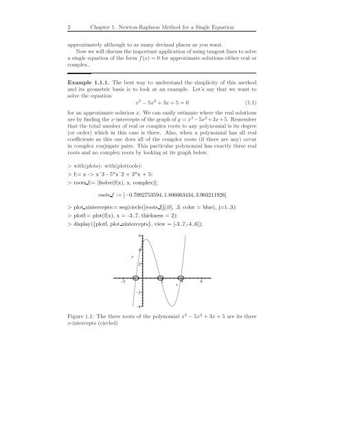
2 Chapter 1. Newton-Raphson Method for a Single Equationapproximately although to as many decimal places as you want.Nowwe will discussthe important applicationofusingtangent lines tosolvea single equation of the form f(x) = 0 for approximate solutions either real orcomplex.Example 1.1.1. The best way to understand the simplicity of this methodand its geometric basis is to look at an example. Let’s say that we want tosolve the equationx 3 −5x 2 +3x+5 = 0 (1.1)for an approximate solution x. We can easily estimate where the real solutionsare by finding the x-intercepts of the graph of y = x 3 −5x 2 +3x+5. Rememberthat the total number of real or complex roots to any polynomial is its degree(or order) which in this case is three. Also, when a polynomial has all realcoefficients as this one does all of the complex roots (if there are any) occurin complex conjugate pairs. This particular polynomial has exactly three realroots and no complex roots by looking at its graph below.> with(plots): with(plottools):> f:= x -> xˆ3 - 5*xˆ2 + 3*x + 5:> roots f:= [fsolve(f(x), x, complex)];roots f := [−0.7092753594,1.806063434,3.903211926]> plot xintercepts:= seq(circle([roots f[j],0], .3, color = blue), j=1..3):> plotf:= plot(f(x), x = -3..7, thickness = 2):> display({plotf, plot xintercepts}, view = [-3..7,-4..6]);6y42–2 2 4 6x–2–4Figure 1.1: The three roots of the polynomial x 3 −5x 2 +3x+5 are its threex-intercepts (circled)
1.1 Geometry of the Newton-Raphson Method 3Figure 1.1 clearly shows that our equation has three real solutions, with anegative one near x = −1 and two positive ones near x = 2 and x = 4. Let’stry to approximate the one near x = 4 as accurately as we can.First, let’s see what fsolve will give us for just the solution near x = 4. Ithas given us all the roots of this polynomial above if we use the complex option.fsolve usesmanyalgorithmssimilartoandincludingtheNewton-Raphsonmethod in combination to approximate solutions both to a single equation ora square system of equations.> fsolve(f(x), x, 3.5..4.5);3.903211926The idea that Raphson had was to take a value of x near x = 4, say x = 5,andput in thetangentline tothegraphofourfunction f(x) atx = 5. Thistangentline goes through the point (5,f(5)) = (5,20) and has slope df (5), wheredxdfis the derivative function of f(x). Now Maple can easily compute both f(5)dxand df (5). The unapply command converts the expressions “diff(f(x), x)” intodxthe derivative function df(x).> f(5);> diff(f(x),x);> df:= unapply(diff(f(x),x),x);> df(5);203x 2 −10x+3df := x → 3x 2 −10x+328So the slope of the tangent line to the graph of y = f(x) at the point (5,20)is 28 and the equation of this tangent line at x = 5 is y−f(5) = dfdx (5)(x−5)or y = 28x−120. Let’s now graph together this tangent line and the originalfunction f(x).> plot guess:= arrow([5,-10], [5,-4.5], .03, .15, .2, color = gold):> plot xint:= arrow([30/7,-10], [30/7,-4.5], .03, .15, .2, color = blue):> plot soln:= arrow([3.9,10], [3.9,2], .03, .15, .2, color = red):> plotfwithtang:= plot([f(x), 28*x - 120], x = 3.5..5.5, color = [red, blue],thickness = [3,2]):
Page 1: Principles of Linear Algebra With M
Page 5: Chapter 1The Newton-RaphsonMethod f
Page 9 and 10: 1.1 Geometry of the Newton-Raphson
Page 15 and 16: 1.2 Examples of the Newton-Raphson
Page 21 and 22: 1.3 When the Newton-Raphson Method
Page 23 and 24: Chapter 2The Newton-RaphsonMethod f
Page 25 and 26: 2.1 Newton-Raphson for Two Equation
Page 33 and 34: 2.1 Newton-Raphson for Three Equati
Page 35 and 36: 2.1 Newton-Raphson for Three Equati
Page 37: 2.1 Newton-Raphson for Three Equati

Principles of Linear Algebra With Maple The NewtonâRaphson ...

You also want an ePaper? Increase the reach of your titles

Delete template?

Save as template?

Principles of Linear Algebra With Maple The NewtonâRaphson ...