Selecting Optimal Distribution Center Placement - Computer ...

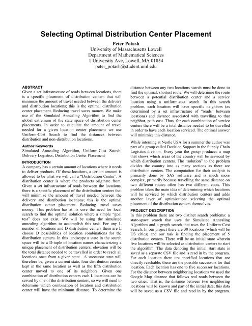
Selecting Optimal Distribution Center PlacementPeter PotashUniversity of Massachusetts LowellDepartment of Mathematical Sciences1 University Ave, Lowell, MA 01854peter_potash@student.uml.eduABSTRACTGiven a set infrastructure of roads between locations, thereis a specific placement of distribution centers that willminimize the amount of travel needed between the deliveryand distribution locations; this is the optimal distributioncenter placement. Reducing travel saves money. We makeuse of the Simulated Annealing Algorithm to find theglobal extremum of the state space of distribution centerplacements. In order to calculate the amount of travelneeded for a given location center placement we useUniform-Cost Search to find the distances betweendistribution and non-distribution locations.Author KeywordsSimulated Annealing Algorithm, Uniform-Cost Search,Delivery Logistics, Distribution Center PlacementINTRODUCTIONA company has a certain amount of locations where it needsto deliver products. Of those locations, a certain amount isallowed to be what we will call a “Distribution Center”. Adistribution center is where the products originate from.Given a set infrastructure of roads between the locations,there is a specific placement of the distribution centers thatwill minimize the amount of travel needed between thedelivery and distribution locations; this is the optimaldistribution center placement. Reducing travel savesmoney. This problem has at its core the need for localsearch to find the optimal solution where a simple “goaltest” does not exist. We will be using the simulatedannealing algorithm to accomplish this task. For any Lnumber of locations and D distribution centers there are Lchoose D possibilities of location combinations for thedistribution centers. In this landscape a state in the searchspace will be a D-tuple of location names characterizing aunique placement of distribution centers; elevation will bethe total distance needed to be travelled in order to reach alllocations once from a given state. A successor state willtherefore be, given a current state, four distribution centerskept in the same location as well as the fifth distributioncenter moved to one of its neighbors. Given onecombination of distribution centers each L locations can beserved by one of the distribution centers, so we will need todetermine which combination of location and distributioncenter will have the minimum distance. To determine thedistance between any two locations search must be done tofind the optimal, shortest route. We will determine the routebetween a potential distribution center and a servicelocation using a uniform-cost search. In this searchproblem, each location will have specific neighbors (asdetermined by a set infrastructure of “roads” betweenlocations) and distance associated with travelling to thatneighbor, path cost. Thus, for each combination of servicecenters there will be a total distance needed to be travelledin order to have each location serviced. The optimal answerwill minimize this distance.While interning at Nestle USA for a summer the author waspart of a group called Decision Support in the Supply ChainLogistics division. Every year the group produces a mapthat shows which areas of the country will be serviced bywhich distribution centers. The “solution” to the problemdivides the country into as many sections as there aredistribution centers. The computation for their analysis isprimarily done by SAS software and is much morecomplex, primarily because travelling the same distance ontwo different routes often has two different costs. Thisproblem takes the main idea of determining which locationswill be serviced by which distribution centers and addsanother layer of optimization: selecting the optimalplacement of the distribution centers themselves.PROJECT DESCRIPTIONIn this problem there are two distinct search problems: astate-space search that uses the Simulated AnnealingAlgorithm and a graph search that uses the Uniform-CostSearch. In our project there are 30 locations (which will beUS cities) and our task is finding the placement of 5distribution centers. There will be an initial state whereinfive locations will be selected as distribution centers to startthe algorithm. The data denoting the initial start state issaved as a separate CSV file and is read in by the program.For each location there are specified locations that aredirectly reachable; these are the possible successors for thatlocation. Each location has one to five successor locations.For the distance between neighboring locations we used theGoogle Map distance that follows real roads between thetwo cities. That is, the distance between two neighboringlocations will be known and part of the initial data; this datawill be saved as a CSV file and read in by the program.

Given a certain state the elevation will be calculated in twoparts. First, we use Uniform-Cost Search to calculate thedistance of the shortest path between each distributioncenter and each location. The name of each location issaved as a CSV file and is read in by the program. The pathcost between successor nodes is the distance of the laneconnecting two neighboring cities. A state in this graphsearchproblem is the current location, the distance travelledto arrive there, the nodes parent, and the action done fromthe parent node to arrive at the current location. Once theUniform-Cost search is completed between all distributioncenters and all locations, each location will have fivedistances associated with it (one for each distributioncenter) and we take the minimum of those distances so thateach location will be serviced by the “closest” distributioncenter (locations that are fixed as distribution centers willhave the trivial distance of zero). It will be the summationof these numbers that will create the total distance(elevation) for each 5 city distribution center combination(state).To begin the Simulated Annealing Algorithm in our statespacesearch the initial state is read in and set to the currentstate. A random successor of the current state is generatedand becomes the next state. This successor state is thecurrent state with one of the distribution locations changedfor one of its neighbors. The elevation (computed asdescribed above) of the current and next state are comparedby subtracting the current elevation from the next elevationgenerally this is done the opposite but in ourimplementation we are actually trying to find lowerelevation). If the next state has a higher elevation than thecurrent state it becomes the current state. Otherwise, thenext state becomes the current state with a probabilitycomputed by the following formula:P = e ( E / T ) (1)Delta E is the elevation change; note it will always benegative here because this probability will only becomputed if the next elevation is higher than the currentelevation. T is the temperature at the current time. At thebeginning of the algorithm time is 1 and it is incrementedby one after each iteration of the algorithm. We set thealgorithm to run until the time became 100, though thealgorithm actually stopped when the temperature became 0.We experimented with two different “cooling” functionsthat mapped time to temperature. They were created theroot of the function is 100 in order for the algorithm to stopat time 100; at time 100 the temperature will be 0. Thedifferent will be discussed in the following sections, butgenerally, functions that produce higher temperatures willresult in a higher probability that next states with a higherelevation will be accepted. Remember that the point of theSimulated Annealing Algorithm is to find the globalextremum without becoming stuck at a local extremum, sothe Simulated Annealing Algorithm allows worse nextstates in order to combat this. As the temperatureapproaches 0, so does the probability that a next state with ahigher elevation will become the current state. Once thealgorithm has finished the current state is presented as thealgorithm’s best attempt at finding the global extremum. Inour application of the algorithm the code prints what itbelieves is the optimal distribution center placement.Different implementations of the Simulated AnnealingAlgorithm can have different stop criteria and differenttypes of cooling functions. While we experimented havingour cooling functions be polynomial functions that haveroots at the time we want the algorithm to terminate, [2]uses a different method. Their cooling function is defined asfollows:t k+1 = T 0 / ( 1 + t k ) (2)Where T 0 is the initial temperature and t k represents thecurrent temperature. Despite this function being oscillatory(as opposed to our monotonically decreasing functions, inthe given time range), it becomes arbitrarily small as kapproaches infinity. However, it never reaches zero.Therefore, the researchers set the stop criterion as havingt k+1 be less than a predetermined value.In [1] the researchers are solving a very similar problem.They are trying to compute which locations should havedistribution centers opened and which customer locationswill be serviced by which distribution location. Like ours,their problem has two layers: a distribution layer and aservice layer. We both approach the distribution layer withthe Simulate Annealing Algorithm. However, they continueusing the Simulated Annealing Algorithm for the servicelayer by creating a “combined” Simulated AnnealingAlgorithm, taking into account distribution capacity andservice demand, whereas we use Uniform-Cost Search inorder to match each location with the closest distributioncenter.ANALYSIS OF RESULTSWe set the 5-tuple (Indianapolis, Cleveland, Buffalo,Boston, Memphis) as the initial state, with an elevation of26,618. We performed the experiment in three variations: 1)The Simulated Annealing Algorithm without ever acceptingworse next states. This makes the algorithm analogous tothe Hill-Climbing Algorithm that always moves “up-hill”,which actually is a lower elevation in our problem. 2) Usingthe function:T = 100 – t (3)as the cooling function. 3) Using the function:T = ( 100 – t ) 3 (4)as the cooling function. Here T is the temperature at a giveniteration defined by t, the time. The time starts at 1 andincrements each iteration. Because the cooling function invariation 3 creates larger temperatures, by (1) it generates ahigher probability that a worse next state will be acceptedas the current state. Running the algorithm 100 iterationstakes 150 seconds, making each iteration roughly 1.5

seconds. This is a problem of 30 choose 5 states, andcalculating each one individually at 1.5 seconds percalculation would take 43 hours 20 minutes. We ran eachalgorithm three times with each variation and noted thefinal elevation delivered by algorithm, the first iterationwhere that elevation was reached, and the highest elevationreached at any point in the algorithm (if different from thefinal elevation) with its first iteration appearance. Theresults are as follows:Variation 1 Result 1 Results 2 Result 3FinalElevationIterationReachedLowestElevation12,276 10,012 12,02087 67 98-- -- --Variation 2 Result 1 Results 2 Result 3FinalElevationIterationReachedLowestElevation10,012 11,894 12,23659 82 93-- -- --Variation 3 Result 1 Results 2 Result 3FinalElevationIterationReachedLowestElevation15,298 14,151 11,58493 97 9612,251; 65 -- 10,893; 53It is clear to see that the third variation which used a thirddegree polynomial cooling function (4) produced the worstresults. This is when comparing final elevation. However,when comparing lowest elevation, the third variation stilldoes worse, but only slightly. Variation one and variationtwo produce very similar results. Due to the lowtemperatures of (3) the algorithm only accepts worse movesif the elevation change between the current and next state issmall. Both variation one and variation two have aninstance where they reach what is likely the state spaceextremum, at the 67 th and 59 th iteration respectively. Thesecond variation, despite being stochastic, never reached anelevation below the final elevation prior to completion ofthe algorithm.DISCUSSIONAs an implementation of the Simulated AnnealingAlgorithm with a high initial temperature is the classicexample, I will first discuss proposed modifications to ouruse of the Simulated Annealing Algorithm to produce betterresults with the third version. Before that, though, we willlook into the inherent flaws. Because the temperature startsoff so high, initially there is a much higher probability thata worse next state will become the current state. Therefore,this variation will have a greater likelihood of spendingmore time at states of low elevation until the temperaturereaches a value wherein the resulting probabilities ofaccepting a worse next states approaches zero. Oursuccessor function produced states with only one locationdifferent, thus producing a relatively minor elevationchange. It might be better suited to produce a completelyrandom successor state. However, we also feel this mightdefeat the meaning of the climbing metaphor and replace itwith more of a pogo stick metaphor. Also, as waspreviously noted, the third variation did reach relatively lowelevations at various iterations of the algorithm, but thesestates were not stored and thus were not outputted as aresult of the algorithm. [3] proposes “The (SimulatedAnnealing) with Best Reserve Mechanism” to overcomethis. In this version of the Simulated Annealing Algorithmthe maximal elevation is always kept track of and iscompared to the final state’s elevation in order to output astate that is truly optimal. An application of this conceptwould have resulted in measurably better results for thethird variation.The first (non-stochastic) variation did well and did notappear to be stuck at a local extremum because the amountof iterations spent at the final elevation when it did notproduce an optimal solution were 13 and 2. While theSimulated Annealing Algorithm uses a certain amount ofiteration to find the area of the state space where the globalextremum is most likely to occur, the hill-climbingalgorithm goes direct toward whatever extremum is closest,be it global or local. By the very nature of the state-space,where states can be uniquely different, though only vary byone out of five cities, local extrema seem relativelyunlikely. Thus, the notion that this variation goes towardany extremum immediately is actually a benefit in thisstate-space search.In terms of time efficiency, using variation one or two, thealgorithm can be run three times, a total of 7 minutes 30seconds and produce a reasonably demonstrated globalextremum, especially when it is kept as the optimalelevation for 41 iterations. This, however, is somewhatdependant on the initial state chosen. Results might nothave been as good if we had started at a much higherelevation (if possible). Ultimately this is superior whencompared to the time needed to calculate each stateindividually – and when compared to the computation timeneeded for a problem of real-world scale – the advantage isundeniable.

CONCLUSIONWhen implementing the Simulated Annealing Algorithm, itis important to focus on a two key factors that may beoverlooked: 1) How will next states be generated? Will theybe completely random or will they follow some thread ofsimilarity from one successor to another? The more randomthe successor, a cooling function with higher temperaturesmight produce better results. 2) Most importantly:Understand the curvature of the state-space. With the wayelevation is defined, what shape does it take? If there seemsto be only one extremum – one can always reach higherelevation from any state – the use of the stochastic aspect ofSimulated Annealing should be limited, if any. Just becausethe Simulated Annealing Algorithm is more complex thanthe Hill-Climbing algorithm it doesn’t necessarily mean it isalways the best choice.ACKNOWLEDGMENTSThe work described in this paper was conducted as part of aFall 2012 Artificial Intelligence course, taught in theComputer Science department of the University ofMassachusetts Lowell by Prof. Fred Martin. We would alsolike to thank Anthony Vardaro for helping us understandclasses and reading in files and Rich Lee for ponderingcooling functions with us.REFERENCES1. Jin, Q., & Li-xin, M. (2009, May). Combined simulatedannealing algorithm for logistics network designproblem. In Intelligent Systems and Applications, 2009.ISA 2009. International Workshop on (pp. 1-4). IEEE.2. Qing-kui, C., Xue-kun, D., & Xian-xin, Z. (2009, May).A Simulated Annealing Methodology to Estate LogisticWarehouse Location Selection and Distribution ofCustomers' Requirement. In Intelligent Systems andApplications, 2009. ISA 2009. International Workshopon (pp. 1-4). IEEE.3. Gao, M., & Tian, J. (2009, May). Modeling andForecasting of Urban Logistics Demand Based onImproved Simulated Annealing Neural Network.In Intelligent Systems, 2009. GCIS'09. WRI GlobalCongress on (Vol. 4, pp. 116-119). IEEE.