2.6 Interpretation of gravity surveys - The Berkeley Course in ...
2.6 Interpretation of gravity surveys - The Berkeley Course in ...
2.6 Interpretation of gravity surveys - The Berkeley Course in ...

Create successful ePaper yourself
Turn your PDF publications into a flip-book with our unique Google optimized e-Paper software.
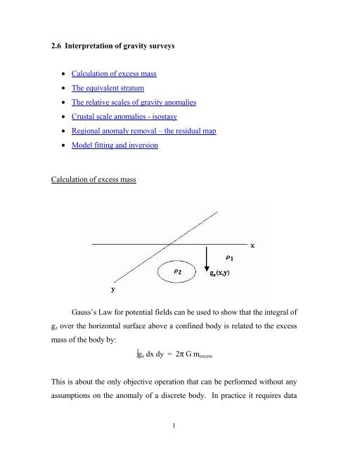
<strong>2.6</strong> <strong>Interpretation</strong> <strong>of</strong> <strong>gravity</strong> <strong>surveys</strong>• Calculation <strong>of</strong> excess mass• <strong>The</strong> equivalent stratum• <strong>The</strong> relative scales <strong>of</strong> <strong>gravity</strong> anomalies• Crustal scale anomalies - isostasy• Regional anomaly removal – the residual map• Model fitt<strong>in</strong>g and <strong>in</strong>versionCalculation <strong>of</strong> excess massGauss’s Law for potential fields can be used to show that the <strong>in</strong>tegral <strong>of</strong>g z over the horizontal surface above a conf<strong>in</strong>ed body is related to the excessmass <strong>of</strong> the body by:g z dx dy = 2π G m excessThis is about the only objective operation that can be performed without anyassumptions on the anomaly <strong>of</strong> a discrete body. In practice it requires data1
from which the anomalies <strong>of</strong> adjacent bodies or structures have beensubtracted.<strong>The</strong> equivalent stratumA fundamental statement <strong>of</strong> non-uniqueness for <strong>gravity</strong> data is that anyobserved <strong>gravity</strong> field on the surface <strong>of</strong> the earth can be represented exactlyby a surface distribution <strong>of</strong> density given by the follow<strong>in</strong>g simple formula:g z (x, y) = 2π G σ (x, y)where σ(x, y) is a ‘surface density’ with the dimension gm cm -2 . Of coursethis is a mathematical relation that implies the existence <strong>of</strong> arbitrary, nonphysical,densities but the implications are obvious. A similar formula can bederived for a physical layer <strong>in</strong> which a lateral variation <strong>of</strong> volume density canrepresent the observed <strong>gravity</strong>. This is a sober<strong>in</strong>g statement about the validity<strong>of</strong> any <strong>gravity</strong> <strong>in</strong>terpretation and it illustrates better than any other model theimportance <strong>of</strong> a sound geological model <strong>in</strong> any <strong>in</strong>terpretation.<strong>The</strong> relative scales <strong>of</strong> <strong>gravity</strong> anomaliesIt is observed <strong>in</strong> field data that there is a roughly l<strong>in</strong>ear relationshipbetween the magnitude <strong>of</strong> an anomaly and its spatial extent or scale. <strong>The</strong>crust <strong>of</strong> the Earth is very <strong>in</strong>homogeneous and there are large-scale variationson the order <strong>of</strong> 100 mgals with scale lengths on the order <strong>of</strong> 100 km. Small2
features such as buried valleys have anomalies <strong>in</strong> the 0.1 to 1.0 mgal rangewith scale lengths <strong>of</strong> 10’s <strong>of</strong> meters.Example:1) US Bouguer Gravity Anomaly Map2) California Bouguer Gravity Anomaly Map3) San Francisco Bouguer Gravity Anomaly Map<strong>The</strong> basic explanation can be seen <strong>in</strong> the anomaly <strong>of</strong> the sphere givenabove <strong>in</strong> section 2.4. <strong>The</strong> maximum anomaly depends on ∆ρ R 3 /z 2 and s<strong>in</strong>cez > R then g z max is always less than or equal to some constant times R. <strong>The</strong>anomaly magnitude scales l<strong>in</strong>early with the size <strong>of</strong> the feature and itsanomaly. (This is fortuitous because it implies that <strong>gravity</strong> can be acquiredwith a spatial sampl<strong>in</strong>g <strong>in</strong>terval dictated by the scale <strong>of</strong> the desired targetwithout alias<strong>in</strong>g caused by small-scale anomalies.)3
Crustal scale anomalies – isostasyMajor geologic features <strong>of</strong> the crust, mounta<strong>in</strong> ranges, sedimentarybas<strong>in</strong>s, ancient cratons, etc. have pronounced <strong>gravity</strong> expressions <strong>in</strong> theBouguer maps. Mounta<strong>in</strong> belts, and plateau areas <strong>in</strong> general, have Bougueranomalies <strong>of</strong> about -100 mgal per kilometer <strong>of</strong> uplift. This is because suchfeatures are ‘float<strong>in</strong>g’ on the viscous higher density upper mantle. <strong>The</strong>y haveroots <strong>of</strong> low-density crustal rock which are the source <strong>of</strong> the negative Bougueranomaly. This float<strong>in</strong>g equilibrium is called isostasy. If perfect isostaticequilibrium is achieved the result<strong>in</strong>g Bouguer anomaly should be exactlyequal to the Bouguer correction that was applied, i.e. 2πG∆ρh. For a typicalcrustal density <strong>of</strong> <strong>2.6</strong>7 we saw <strong>in</strong> section 2.2 that this is 0.118 mgal/m or 118mgal/km - just about what is observed.Regional anomaly removal - the residual map<strong>The</strong> anomaly amplitude vs. scale length relationship shows that anydesired anomaly will almost <strong>in</strong>evitably be superimposed on a bigger anomalywith a bigger spatial scale. To <strong>in</strong>terpret the desired feature the larger scaleanomaly should be subtracted. This is called removal <strong>of</strong> the regional anomalyand the rema<strong>in</strong>der is called the residual. <strong>The</strong> process <strong>of</strong> isolat<strong>in</strong>g the localanomaly is probably the most challeng<strong>in</strong>g aspect <strong>of</strong> <strong>gravity</strong> <strong>in</strong>terpretation.<strong>The</strong> cont<strong>in</strong>uum <strong>of</strong> scales makes it very difficult to unambiguously separate adesired (suspected?) feature without know<strong>in</strong>g the answer! A mathematical4
statement <strong>of</strong> the problem is that one has to apply a high pass filter withoutknow<strong>in</strong>g the spectrum <strong>of</strong> the target.In practice the process used is subjective and critically dependent onthe geologic model that is assumed. Some <strong>of</strong> the specific techniques that areemployed area) subtraction <strong>of</strong> a plane or higher order polynomial that is fitted to thedata outside the area <strong>of</strong> <strong>in</strong>terest.b) rigorous filter<strong>in</strong>g <strong>of</strong> the two-dimensional spatial frequency spectrumwith a high-pass, possibly directional, filter.c) wavelet filter.Example:1) Isostatic Residual Gravity Map <strong>of</strong> the US2) Isostatic Residual Gravity Map <strong>of</strong> California5
3) Isostatic Residual Gravity Map <strong>of</strong> the San Francisco Bay AreaThis map is from USGS web pageFor Additional Information see the map: Roberts, C.W., and Jachens, R.C., 1993, Isostaticresidual <strong>gravity</strong> map <strong>of</strong> the San Francisco Bay area, California: U.S. Geological SurveyGeophysical Investigations Map GP-1006. Available from the USGS--Information Services,Box 25286, Bldg. 810, Denver Federal Center, Denver, CO 80225 303 236-4210.Model fitt<strong>in</strong>g and <strong>in</strong>version<strong>The</strong> f<strong>in</strong>al step <strong>in</strong> <strong>in</strong>terpretation is the fitt<strong>in</strong>g <strong>of</strong> a model the simulateddata from which matches the observed residual Bouguer map. <strong>The</strong> process isusually carried out <strong>in</strong>teractively - the <strong>in</strong>terpreter alters the parameters <strong>of</strong> anassumed model until a good visual fit is obta<strong>in</strong>ed with the data. In general theresults are usually as good as the appropriateness <strong>of</strong> the assumed geologicmodel.In the past few years great advances have been made <strong>in</strong> automatedmodel fitt<strong>in</strong>g. In this process the parameters <strong>of</strong> an assumed model are variedsystematically by an algorithm until the model ‘data’ matches the observeddata <strong>in</strong> some least squares sense. <strong>The</strong>se are called <strong>in</strong>version techniques andthey will be discussed <strong>in</strong> a later section <strong>of</strong> this course.6