Magnetic Field Induced Semimetal-to-Canted-Antiferromagnet ...
Magnetic Field Induced Semimetal-to-Canted-Antiferromagnet ...
Magnetic Field Induced Semimetal-to-Canted-Antiferromagnet ...

Create successful ePaper yourself
Turn your PDF publications into a flip-book with our unique Google optimized e-Paper software.
<strong>Magnetic</strong> <strong>Field</strong> <strong>Induced</strong><br />
<strong>Semimetal</strong>-<strong>to</strong>-<strong>Canted</strong>-<strong>Antiferromagnet</strong><br />
Transition on the Honeycomb Lattice<br />
Diplomarbeit<br />
von<br />
Martin Helmut Bercx<br />
vorgelegt bei<br />
Professor Dr. F. F. Assaad<br />
Institut für Theoretische Physik und Astrophysik<br />
Julius-Maximilians-Universität<br />
Würzburg<br />
14. April 2008
Contents<br />
1 Introduction 5<br />
2 Mean <strong>Field</strong> Treatment 7<br />
2.1 The model Hamil<strong>to</strong>nian . . . . . . . . . . . . . . . . . . . . . . . . . . . . . 7<br />
2.2 Examination of the transversal susceptibility . . . . . . . . . . . . . . . . . 9<br />
2.3 Mean field decoupling . . . . . . . . . . . . . . . . . . . . . . . . . . . . . . 13<br />
2.4 Meanfield phase transition . . . . . . . . . . . . . . . . . . . . . . . . . . . . 16<br />
2.5 Spectral function . . . . . . . . . . . . . . . . . . . . . . . . . . . . . . . . . 18<br />
3 Functional Integral Formulation 25<br />
3.1 The partition function as a path integral over imaginary time . . . . . . . . 25<br />
3.2 Introduction of the auxiliary field . . . . . . . . . . . . . . . . . . . . . . . . 27<br />
3.3 Discrete Hubbard-Stra<strong>to</strong>novich transformation . . . . . . . . . . . . . . . . 28<br />
3.4 Formulation of the partition function . . . . . . . . . . . . . . . . . . . . . . 29<br />
4 The Projec<strong>to</strong>r QMC Method 31<br />
4.1 The trial wave function . . . . . . . . . . . . . . . . . . . . . . . . . . . . . 31<br />
4.2 Observables in the PQMC algorithm . . . . . . . . . . . . . . . . . . . . . . 33<br />
4.2.1 Equal time Green function G(τ) . . . . . . . . . . . . . . . . . . . . 33<br />
4.2.2 Imaginary time displaced Green function G(τ′, τ) . . . . . . . . . . . 35<br />
4.2.3 Efficient calculation of G(τ′, τ) . . . . . . . . . . . . . . . . . . . . . 36<br />
5 Outline of the Monte Carlo Technique 39<br />
5.1 The Monte Carlo sampling . . . . . . . . . . . . . . . . . . . . . . . . . . . 39<br />
5.1.1 Implementation in the algorithm . . . . . . . . . . . . . . . . . . . . 41<br />
5.2 The PQMC algorithm . . . . . . . . . . . . . . . . . . . . . . . . . . . . . . 42<br />
5.2.1 Efficient realization . . . . . . . . . . . . . . . . . . . . . . . . . . . . 44<br />
6 Results 47<br />
6.1 Static observables . . . . . . . . . . . . . . . . . . . . . . . . . . . . . . . . . 47<br />
6.2 Excitation spectra . . . . . . . . . . . . . . . . . . . . . . . . . . . . . . . . 48<br />
3
Contents<br />
7 Conclusion 55<br />
Appendix 57<br />
A Lattice structure . . . . . . . . . . . . . . . . . . . . . . . . . . . . . . . . . 57<br />
B Singular Value Decompostion . . . . . . . . . . . . . . . . . . . . . . . . . . 59<br />
C Metropolis scheme . . . . . . . . . . . . . . . . . . . . . . . . . . . . . . . . 60<br />
D Approximation of tanh(x) . . . . . . . . . . . . . . . . . . . . . . . . . . . . 61<br />
Bibliography 61<br />
Erklärung 67<br />
4
1 Introduction<br />
The study of systems with reduced dimensionality has been revitalized by the recent re-<br />
alization of graphene sheets. Since then graphene has triggered intensive research equally<br />
on the theoretical and experimental sides [28]. The spectrum of scientific research ranges<br />
from studies of BCS-BEC crossover of the attractive Hubbard model [11] <strong>to</strong> the very re-<br />
cent discovery of giant intrinsic carrier mobilities in single and bilayer graphene [10].<br />
To form graphene carbon a<strong>to</strong>ms crystallize in the honeycomb lattice. The electrons interact<br />
with the resulting periodic potential and display an unprecedented low energy behaviour.<br />
The excitations satisfy the massless Dirac equation as opposed <strong>to</strong> the Schrödinger equa-<br />
tion which usually describes the electronic properties of materials. These massless Dirac<br />
fermions allow for several analogies with QED. As a consequence of the bipartite nature of<br />
the honeycomb lattice one may introduce a spin index called pseudospin <strong>to</strong> discriminate<br />
between the sublattices and evoke the concept of chirality [32].<br />
Although the role of many-body interactions in graphene remains unclear so far modi-<br />
fications of the band structure which cannot be explained in terms of a single electron<br />
picture have been found. The observed kinks near the Fermi energy were atrributed <strong>to</strong><br />
electron-phonon and elctron-plasmon interactions [29].<br />
In this thesis the Hubbard model on the honeycomb lattice in an external magnetic field<br />
is studied. The tight-binding band diplays two inequivalent cone shaped singularities,<br />
the so called Dirac points which are located in the Brillouin zone where upper and lower<br />
band <strong>to</strong>uch each other (Fig. 1.1). Consequently, in the honeycomb lattice at half filling<br />
the Fermi surface geometry is pointlike and the Fermi surface density of states vanishes<br />
linearly. A spin density wave instability according <strong>to</strong> the S<strong>to</strong>ner criterion therefore does<br />
not develop in the honeycomb lattice at an infinitesimally small U. It has been shown<br />
that the symnetry breaking phase transtions occurs at a finite Uc and coincides with a<br />
Mott-Hubbard transition [13].<br />
Introducing a magnetic field changes the Fermi surface geometry <strong>to</strong>wards a circular-like<br />
shape and generates a finite density of states at the Fermi level. Nesting between up and<br />
down spin Fermi surface leads <strong>to</strong> a S<strong>to</strong>ner like instability <strong>to</strong>wards canted antiferromagnetic<br />
order.<br />
Since the S<strong>to</strong>ner criterion is a mean-field result a saddle point approximation should cap-<br />
ture much of the underlying physics. We use this approach as a starting point. Treating<br />
the electron-electron interaction correctly with numerical quantum Monte Carlo simula-<br />
5
1 Introduction<br />
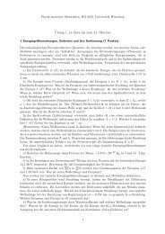
Figure 1.1: Pho<strong>to</strong>emission intensity pattern of single (a) and bilayer (b) graphene along the high<br />
symmetry direction Γ-K-M-Γ which reflects its band structure. The dashed blue lines have been<br />
included for comparison with a density functional calculation. The figure is taken from [12].<br />
tions this picture is confirmed <strong>to</strong> a good degree. A critical U of order Uc ≈ 4−5 is observed<br />
in accordance with what has been found out previously [13]. We show that under the ac-<br />
tion of the field the critical U is lowered from the strong interaction of the free system<br />
<strong>to</strong>wards an experimentally more accesible region. The transition takes the semimetal <strong>to</strong><br />
an canted antiferromagnet which is heralded by the opening of a gap in the excitation<br />
spectrum.<br />
The thesis is organized as follows. In chapter one the model Hamil<strong>to</strong>nian is introduced<br />
and is studied on a mean field level. By studying the transverse susceptibility we show<br />
that under the action of a vertical magnetic field the system gets logarithmically insta-<br />
ble. This chapter concludes with the evaluation of the single-particle spectral function<br />
and the concomitant density of states. The chapters two and three are rather technical<br />
and include the foundations for the numerical treatment of the many-body problem. The<br />
quantum Monte Carlo approach, more precisely the projec<strong>to</strong>r quantum Monte Carlo al-<br />
gorithm, is explained and big emphasize lies on the stable computation of observables.<br />
Finally, in chapter four the numerically obtained static and dynamic results which include<br />
the staggered magnetization and the excitation spectra are discussed.<br />
6
2 Mean <strong>Field</strong> Treatment<br />
The standard model <strong>to</strong> describe the electronic and magnetic properties of correlated elec-<br />
trons on a lattice is the Hubbard model. Being conceptually simple this model incorpo-<br />
rates two opposing trends: electron hopping which tends <strong>to</strong> delocalize the electrons and<br />
electron-electron interactions leading <strong>to</strong> localization. In this chapter the hexagonal lattice<br />
is discussed in the context of the Hubbard model.<br />
The complexity of many particle problems can be dramatically reduced by a molecular<br />
field approximation. This approximation replaces the electron-electron interaction term<br />
in the Hamil<strong>to</strong>nian with effective one body expressions, thereby neglecting fluctuations of<br />
the particle opera<strong>to</strong>rs. The idea is that fluctuations only play the role of small oscillations<br />
around the mean value of a physical observable. Given this simplification the interaction<br />
acts like a space and spin dependent external field, the molecular field. The molecular<br />
field is the one which minimizes the free energy. The problem is thus tractable on a mean<br />
field level, that is one may diagonalize the Hamil<strong>to</strong>nian and describe phase transitions.<br />
The prize we have <strong>to</strong> pay is the loss of information since effects governed by real electron<br />
correlations are lost. On the other hand the physical significance of the mean field solution<br />
is limited, since the assumptions needed <strong>to</strong> decouple the interaction term essentially are<br />
reconfirmed in the end. Nevertheless the mean field treatment serves a valuable starting<br />
point for more detailed analytical techniques or numerical approaches like the Quantum<br />
Monte Carlo method. The molecular field method is a self-consistent approximation and<br />
helps <strong>to</strong> understand fundamental properties of the hexagonal lattice. It is used <strong>to</strong> quali-<br />
tatively describe the paramagnetic and antiferromagnetic phase and <strong>to</strong> extract the single<br />
particle spectral function.<br />
2.1 The model Hamil<strong>to</strong>nian<br />
The generic Hamil<strong>to</strong>n opera<strong>to</strong>r in the Hubbard model is<br />
H = HT + HI = − �<br />
(ti,j − µ)ĉ †<br />
i,σĉj,σ + U �<br />
ˆni,↑ˆni,↓ . (2.1)<br />
i,j,σ<br />
Here ti,j are hopping integrals, U is the on-site repulsion, µ is the chemical potential<br />
and ˆni,σ = ĉ †<br />
i,σ ĉi,σ is the electron density opera<strong>to</strong>r. In the following we assume strongly<br />
localized Wannier orbitals that we restrict ourselves <strong>to</strong> hopping processes <strong>to</strong> the nearest<br />
i<br />
7
2 Mean <strong>Field</strong> Treatment<br />
neighbours, with ti,j ≡ t. In the case of half-filling µ = 0.<br />
The lattice vec<strong>to</strong>rs are<br />
⎛<br />
a1 = a ⎝ 1/2<br />
⎞<br />
⎛<br />
√ ⎠<br />
3/2<br />
a2 = a ⎝ 1<br />
⎞<br />
⎠ ,<br />
0<br />
(2.2)<br />
a is the distance of neighbouring sites on sublattice A and B. The term of kinetic energy<br />
contains the hopping processes on the bipartite lattice and it reads<br />
with<br />
HT = −t �<br />
= −t �<br />
H11 = H22 = 0<br />
(â †<br />
R,σ ˆ bR,σ + â †<br />
R,σ ˆ bR+a2−a1,σ + â †<br />
R,σ ˆ bR−a1,σ) + h.c.<br />
R, σ, â∈A, ˆb∈B �<br />
â<br />
k,σ<br />
†<br />
k,σ ˆb †<br />
�<br />
k,σ<br />
⎡<br />
⎣ H11 H12<br />
H21 H22<br />
⎤ ⎛<br />
⎦<br />
⎝ âk,σ<br />
ˆ bk,σ<br />
⎞<br />
⎠ , (2.3)<br />
H12 = H ∗ 21 = 1 + e ık(a2−a1) + e −ıka1 (2.4)<br />
Upon diagonalization of the Hermitian Hamil<strong>to</strong>n matrix one gets the two tight binding<br />
bands 1 (Fig. 2.1)<br />
Γ±(k) = ± � 3 + 2 cos k(a2 − a1) + 2 cos ka1 + 2 cos ka2 . (2.5)<br />
Figure 2.1: Energy spectrum Γ(kx, ky) of the two dim. hexagonal lattice, based on the assumption<br />
of free electrons (tight-binding model). Valence and conduction band <strong>to</strong>uch each other at the socalled<br />
Dirac points and the energy gap vanishes.<br />
8<br />
1 Here and in the following we set t ≡ 1.
2.2 Examination of the transversal susceptibility<br />
2.2 Examination of the transversal susceptibility<br />
In this section we concentrate on possible magnetic instabilities of the free Hamil<strong>to</strong>-<br />
nian under the action of a vertical magnetic field (conventionally chosen as B = Bez),<br />
H = HT + Hfield. <strong>Magnetic</strong> order is heralded by the divergence of the appropriate mag-<br />
netic susceptibility when the temperature goes <strong>to</strong> zero. Here we look at the possibility of<br />
staggered antiferromagnetic order in the transversal plane of the lattice.<br />
The Hamil<strong>to</strong>nian can easily be diagonalized <strong>to</strong><br />
H = HT + B<br />
2<br />
= �<br />
k,σ<br />
� �<br />
pσˆnσ<br />
A,B k,σ<br />
Eγ (k, σ)ˆγ † ˆγ + Eη(k, σ) ˆη † ˆη (2.6)<br />
The quasi particle energies 2 are Eγ,η(k, σ) = B<br />
2 pσ ∓ Γ(k), pσ = ±1, and the particle oper-<br />
a<strong>to</strong>rs are<br />
ˆγ = 1<br />
�<br />
√ â +<br />
2<br />
Γ<br />
�<br />
ˆb ,<br />
H21<br />
ˆη = 1<br />
�<br />
−Γ<br />
√ â +<br />
2 H12<br />
ˆ �<br />
b ,<br />
â = 1<br />
�<br />
√ ˆγ −<br />
2<br />
Γ<br />
�<br />
ˆη ,<br />
H21<br />
� �<br />
ˆ<br />
1 Γ<br />
b = √2 ˆγ + ˆη . (2.7)<br />
H12<br />
Correlation functions like the single particle Green function or the susceptibility are 2 × 2<br />
matrices as a consequence of the two sublattices used <strong>to</strong> describe the hexagonal lattice.<br />
In particular the tensorial nature of the transversal spin susceptibility χ +− lies in the two<br />
orbitals per unit cell and is not due <strong>to</strong> anisotropy effects. The tensor of the transversal<br />
susceptibility is:<br />
χ +− (q, ω) =<br />
⎛<br />
⎝ χ+−<br />
AA χ+−<br />
AB<br />
χ +−<br />
BA χ+−<br />
BB<br />
⎞<br />
⎠ (2.8)<br />
From now on we are only concerned with the static case, χ +− (q) ≡ χ +− (q, ω = 0). Within<br />
the Matsubara formalism 3 the components are defined as<br />
χ +−<br />
� β<br />
µ,ν (q) =<br />
0<br />
dτ〈S + µ (q, τ)S − ν (-q, 0)〉 . (2.9)<br />
2 Here, Γ ≡ Γ+.<br />
3 In this work, the modified Heisenberg picture is employed <strong>to</strong> describe the time evolution in imaginary<br />
time, that is A(τ) = e Hτ A(0)e −Hτ . [1],[3]. For notational clarity, we have set ¯h ≡ 1 in the whole text.<br />
9
2 Mean <strong>Field</strong> Treatment<br />
The indices are µ = A, B, ν = A, B and the spin raising and lowering opera<strong>to</strong>rs are<br />
S +(−)<br />
µ (q) = 1<br />
√ N<br />
�<br />
k<br />
ĉ † µ k,↑(↓) ĉµ k+q,↓(↑) , (2.10)<br />
with the particle opera<strong>to</strong>rs ĉA = â, ĉB = ˆ b on the sublattices. For later use we note that<br />
χ +−<br />
µ,µ = χ +−<br />
ν,ν and χ +−<br />
µ,ν = (χ +−<br />
ν,µ ) ∗ , in the static (ω = 0) case χ +−<br />
µ,ν = χ +−<br />
ν,µ . The transversal<br />
magnetization on orbital µ amounts <strong>to</strong><br />
m xy<br />
µ = �<br />
α=µ,ν<br />
χ +−<br />
µ,αB xy<br />
α . (2.11)<br />
B xy<br />
α are the orbital components of a transversal magnetic field. For B xy<br />
µ = −B xy<br />
ν we<br />
obtain the antiferromagnetic susceptibility χ +−<br />
µµ − χ +−<br />
µν , for B xy<br />
µ = B xy<br />
ν the ferromagnetic<br />
susceptibility χ +−<br />
µµ + χ +−<br />
µν . Since the ordering takes places within the orbitals at formally<br />
the same lattice point it can be characterized with the wave vec<strong>to</strong>r q = 0. However, for<br />
reasons of generality we keep the vec<strong>to</strong>r q during the calculation and in the end we set it<br />
equal <strong>to</strong> zero.<br />
The components χ +−<br />
µ,ν (q) may be calculated applying Wick’s theorem and using the quasiparticle<br />
expressions for ˆγ und ˆη (2.7):<br />
χ +−<br />
µ,ν (q) =<br />
=<br />
=<br />
=<br />
=<br />
=<br />
� β<br />
dτ〈S<br />
0<br />
+ µ (q, τ)S − ν (−q, 0)〉 (2.12)<br />
� β 1<br />
dτ<br />
N 0<br />
�<br />
〈ĉ<br />
k,k′<br />
† µk,↑ (τ)ĉµk+q,↓ (τ)ĉ† νk′,↓<br />
(0)ĉνk′−q,↑ (0)〉<br />
� β 1<br />
dτ<br />
N 0<br />
�<br />
〈ĉ<br />
k,k′<br />
† µk,↑ (τ)ĉµk+q,↓ (τ)〉〈ĉ† νk′,↓<br />
(0)ĉνk′−q,↑ (0)〉<br />
+〈ĉ † µk,↑ (τ)ĉνk′−q,↑ (0)〉〈ĉµk+q,↓ (τ)ĉ† νk′,↓ (0)〉<br />
� β<br />
1<br />
N<br />
1<br />
4N<br />
1<br />
4N<br />
0<br />
� β<br />
0<br />
� β<br />
0<br />
dτ �<br />
〈ĉ † µk,↑ (τ)ĉνk,↑ (0)〉〈ĉµk+q,↓ (τ)ĉ† νk+q,↓ (0)〉<br />
k<br />
dτ ��<br />
k<br />
dτ �<br />
k<br />
〈ˆγ † (τ)ˆγ(0)〉k,↑ ± 〈ˆη † (τ)ˆη(0)〉k,↑<br />
��<br />
〈ˆγ(τ)ˆγ † (0)〉k+q,↓ ± 〈ˆη(τ)ˆη † (0)〉k+q,↓<br />
�<br />
〈ˆγ † (τ)ˆγ(0)〉k,↑〈ˆγ(τ)ˆγ † (0)〉k+q,↓ ± 〈ˆγ † (τ)ˆγ(0)〉k,↑〈ˆη(τ)ˆη † (0)〉k+q,↓<br />
±〈ˆη † (τ)ˆη(0)〉k,↑〈ˆγ(τ)ˆγ † (0)〉k+q,↓ + 〈ˆη † (τ)ˆη(0)〉k,↑〈ˆη(τ)ˆη † (0)〉k+q,↓<br />
Here, ”+” stands for µ = ν and −” for µ �= ν; the first term in line three is equal <strong>to</strong> zero<br />
since the Hamil<strong>to</strong>nian (2.6) does not include spin flip processes. The antiferromagnetic<br />
10<br />
�<br />
.<br />
�
and ferromagnetic susceptibilities are therefore written as<br />
χ +−<br />
µµ − χ +−<br />
µν<br />
=<br />
χ +−<br />
µµ + χ +−<br />
µν<br />
=<br />
� β 1<br />
2N 0<br />
� β 1<br />
2N 0<br />
dτ �<br />
k<br />
dτ �<br />
k<br />
2.2 Examination of the transversal susceptibility<br />
(2.13)<br />
�<br />
�<br />
〈ˆγ † (τ)ˆγ(0)〉k,↑〈ˆη(τ)ˆη † (0)〉k+q,↓ + 〈ˆη † (τ)ˆη(0)〉k,↑〈ˆγ(τ)ˆγ † (0)〉k+q,↓<br />
(2.14)<br />
�<br />
.<br />
�<br />
〈ˆγ † (τ)ˆγ(0)〉k,↑〈ˆγ(τ)ˆγ † (0)〉k+q,↓ + 〈ˆη † (τ)ˆη(0)〉k,↑〈ˆη(τ)ˆη † (0)〉k+q,↓<br />
We proceed <strong>to</strong> calculate the ferromagnetic susceptibility, introducing the short notation<br />
ĉi with i = γ, η referring <strong>to</strong> the ˆγ and ˆη opera<strong>to</strong>rs.<br />
χ +−<br />
µµ + χ +−<br />
µν<br />
=<br />
=<br />
=<br />
=<br />
q=0<br />
=<br />
=<br />
� β 1<br />
2N 0<br />
1<br />
2N<br />
� β<br />
0<br />
1 �<br />
2N<br />
1<br />
2N<br />
1<br />
2N<br />
k<br />
�<br />
k<br />
�<br />
k<br />
1 �<br />
2NB<br />
k<br />
dτ �<br />
k<br />
dτ �<br />
�<br />
i=γ,η<br />
�<br />
i=γ,η<br />
�<br />
i=γ,η<br />
k<br />
�<br />
e β<br />
i=γ,η<br />
In line four the Fermi function fi(k) =<br />
�<br />
〈ĉ †<br />
†<br />
i (τ)ĉi(0)〉k,↑〈ĉi(τ)ĉ i<br />
i=γ,η<br />
(0)〉k+q,↓<br />
�<br />
e<br />
i=γ,η<br />
τ<br />
� �<br />
Ei(k,↑)−Ei(k+q,↓)<br />
〈ĉ †<br />
i ĉi〉k,↑<br />
�<br />
1 − 〈ĉ †<br />
i ĉi〉k+q,↓<br />
�<br />
� �<br />
Ei(k,↑)−Ei(k+q,↓)<br />
− 1<br />
i ĉi〉k,↑e βEi(k+q,↓) †<br />
〈ĉ i ĉi〉k+q,↓<br />
Ei(k, ↑) − Ei(k + q, ↓) 〈ĉ†<br />
fi(k + q, ↓) − fi(k, ↑)<br />
Ei(k, ↑) − Ei(k + q, ↓)<br />
fi(k, ↓) − fi(k, ↑)<br />
Ei(k, ↑) − Ei(k, ↓)<br />
� �� �<br />
B<br />
�<br />
�<br />
fi(k, ↓) − fi(k, ↑)<br />
(2.15)<br />
1<br />
e βE i (k) +1 and Ei(k) = pσ B<br />
2 +Γi was introduced. The<br />
parenthesis in the last line denote the magnetization in z-direction for both bands j = γ, η.<br />
This expression is zero for vanishing external field and at a given field it approaches unity<br />
for T → 0 (Fig.2.2).<br />
11
2 Mean <strong>Field</strong> Treatment<br />
We now evaluate the antiferromagnetic susceptibility, again using the notation ĉi, i = γ, η.<br />
χ +−<br />
µµ − χ +−<br />
µν<br />
=<br />
=<br />
=<br />
=<br />
q=0<br />
=<br />
1<br />
2N<br />
� β<br />
0<br />
dτ �<br />
k<br />
� β 1<br />
dτ<br />
2N 0<br />
�<br />
k<br />
1 �<br />
2N<br />
k<br />
1 �<br />
2N<br />
k<br />
1 �<br />
2N<br />
k<br />
�<br />
i=γ,η<br />
j=γ,η<br />
i�=j<br />
�<br />
i=γ,η<br />
j=γ,η<br />
i�=j<br />
�<br />
i=γ,η<br />
j=γ,η<br />
i�=j<br />
�<br />
i=γ,η<br />
j=γ,η<br />
i�=j<br />
�<br />
i=γ,η<br />
j=γ,η<br />
〈ĉ †<br />
†<br />
i (τ)ĉi(0)〉k,↑〈ĉj(τ)ĉ j (0)〉k+q,↓<br />
e τ<br />
� �<br />
Ei(k,↑)−Ej(k+q,↓)<br />
〈ĉ †<br />
i ĉi〉k,↑<br />
�<br />
1 − 〈ĉ †<br />
jĉj〉k+q,↓ �<br />
i�=j<br />
�<br />
Ei(k,↑)−Ej(k+q,↓)<br />
e β<br />
�<br />
− 1<br />
Ei(k, ↑) − Ej(k + q, ↓) 〈ĉ†<br />
fj(k + q, ↓) − fi(k, ↑)<br />
Ei(k, ↑) − Ej(k + q, ↓)<br />
i ĉi〉k,↑e βEj(k+q,↓) †<br />
〈ĉ jĉj〉k+q,↓ fj(k, ↓) − fi(k, ↑)<br />
. (2.16)<br />
Ei(k, ↑) − Ej(k, ↓)<br />
The denomina<strong>to</strong>r can be written as<br />
Ei(k, ↑)−Ej(k, ↓) = B<br />
2 +Γi− � − B<br />
2 +Γj<br />
� �<br />
B<br />
= B+Γi−Γj = B−2Γj = 2<br />
2 −Γj<br />
�<br />
,(2.17)<br />
since Γj = −Γ, +Γ for j = γ, η. The enumera<strong>to</strong>r is<br />
fj(k, ↓) − fi(k, ↑) =<br />
We finally get with ξj = B<br />
2<br />
Γi=−Γj<br />
=<br />
=<br />
− Γj<br />
j=γ,η<br />
1<br />
e β<br />
�<br />
B<br />
− 2 +Γj<br />
1<br />
� −<br />
+ 1 e β<br />
�<br />
B<br />
2 +Γi<br />
�<br />
+ 1<br />
e −β<br />
�<br />
B<br />
− 2 +Γj<br />
�<br />
1 + e −β<br />
�<br />
B<br />
− 2 +Γj<br />
1<br />
� −<br />
e −β<br />
�<br />
B<br />
− 2 +Γj<br />
�<br />
+ 1<br />
e −β<br />
�<br />
B<br />
− 2 +Γj<br />
�<br />
− 1<br />
1 + e −β<br />
�<br />
B<br />
− 2 +Γj<br />
�<br />
β<br />
�<br />
B<br />
�<br />
� = tanh − Γj<br />
2 2 �<br />
.<br />
(2.18)<br />
χ +−<br />
µµ − χ +−<br />
µν = 1 1 � �<br />
�<br />
1<br />
β<br />
�<br />
B<br />
�<br />
� � tanh − Γj<br />
2 N<br />
B<br />
k j=γ,η 2 2 − Γj<br />
2 2 �<br />
= 1 1 � �<br />
�<br />
1 β<br />
� �<br />
tanh ξj<br />
2 N 2ξj 2<br />
k j=γ,η<br />
�<br />
.<br />
� � ��<br />
β<br />
Using the approximation (in the appendix) for tanh 2<br />
ξj ,<br />
(2.19)<br />
�<br />
χ +−<br />
µµ − χ +−<br />
�<br />
µν (T ) ≈ 1<br />
2<br />
�<br />
�<br />
W<br />
�<br />
DOS(ɛF,j) ln .<br />
2T<br />
(2.20)<br />
12
χ FM<br />
0.2<br />
0.15<br />
0.1<br />
0.05<br />
0<br />
0 0.5 1 1.5 2<br />
(a)<br />
T<br />
“<br />
χ +−<br />
µµ + χ +−<br />
µν<br />
”<br />
(T )<br />
B = 0.00<br />
B = 0.25<br />
B = 0.50<br />
B = 0.70<br />
B = 1.00<br />
χ AFM<br />
0.8<br />
0.7<br />
0.6<br />
0.5<br />
0.4<br />
0.3<br />
0.2<br />
0.1<br />
2.3 Mean field decoupling<br />
0<br />
0 0.5 1 1.5 2<br />
(b)<br />
T<br />
“<br />
χ +−<br />
µµ − χ +−<br />
µν<br />
B = 0.00<br />
B = 0.25<br />
B = 0.50<br />
B = 0.70<br />
B = 1.00<br />
f(T)=a + b log(c/T)<br />
”<br />
(T )<br />
Figure 2.2: Numerical evaluation of the ferromagnetic and antiferromagnetic susceptibility, for<br />
varying fields B. The logarithmic divergence of χ +−<br />
AF M (T ) as T → 0 is visualized by a logarithmic<br />
fitting function f(T ) (a = 0.27, b = 0.15, c = 0.5).<br />
Thus,<br />
�<br />
χ +−<br />
µµ −χ +−<br />
�<br />
µν (T ) diverges logarithmically as T goes <strong>to</strong> zero. (Fig.2.2) This behaviour<br />
is signaled already in the Lindhard type result for the antiferromagnetic susceptibility,<br />
(2.16). We consider the nesting condition, which is known <strong>to</strong> be<br />
ɛ(k + Q nest) = −ɛ(k) . (2.21)<br />
In our case antiferromagnetic order sets in at Q nest = 0 so the nesting condition now reads<br />
Ei(k, ↑) = −Ej(k, ↓) (2.22)<br />
which is obviously fulfilled. That is, we describe the hexagonal lattice being on the edge<br />
of staggered antiferromagnetic order as a consequence of the nesting of its up and down<br />
Fermisurface. The ordering is predicted <strong>to</strong> occur at a small non-zero interaction U (see<br />
section 2.4).<br />
2.3 Mean field decoupling<br />
We now consider the following Hubbard model with on-site interaction and external mag-<br />
netic field:<br />
H = Hhopping + Hfield + HI<br />
= −t � ��<br />
1 + e ık(a2−a1)<br />
�<br />
−ıka1 + e<br />
+ B<br />
2<br />
k,σ<br />
� �<br />
pσˆnσ + U � �<br />
�<br />
ˆni↑ − 1<br />
� �<br />
ˆni↓ −<br />
2<br />
1<br />
�<br />
2<br />
A,B k,σ<br />
A,B<br />
i<br />
â †<br />
k,σ ˆ �<br />
bk,σ + 1 + e −ık(a2−a1)<br />
�<br />
ıka1 + e ˆb †<br />
k,σâk,σ �<br />
. (2.23)<br />
13
2 Mean <strong>Field</strong> Treatment<br />
In order <strong>to</strong> arrive at an effective molecular field Hamil<strong>to</strong>nian we make two assumptions:<br />
1. The biquadratic term is rewritten as:<br />
HI = U � �<br />
�<br />
ˆni↑ −<br />
A,B i<br />
1<br />
� �<br />
ˆni↓ −<br />
2<br />
1<br />
�<br />
= −<br />
2<br />
U � � �<br />
(ˆni,↑ − ˆni,↓)<br />
2<br />
A,B i<br />
2 − 1 �<br />
= − U � � �<br />
(2<br />
2<br />
ˆ S z i,α) 2 �<br />
− 1 = − 2 � � � �2 U ˆSi,α + UN . (2.24)<br />
3<br />
A,B<br />
i<br />
In this notation the spin-rotational invariance, that is the invariance of HI under<br />
A,B<br />
simultaneous rotation of all spins is explicitely used.<br />
2. The transversal component mx of the magnetization �m is assumed <strong>to</strong> be staggered,<br />
that is alternating on the sublattices A and B: mx,A = −mx,B. Put differently, with<br />
the index α = 0, 1 which labels the orbitals in the unit cell:<br />
.<br />
�mα =<br />
�<br />
mx(−1) α �<br />
, 0, mz<br />
i<br />
(2.25)<br />
Therefore we assume the magnetization �m <strong>to</strong> have a constant component mz parallel <strong>to</strong><br />
the field axis and a staggered component mx(−1) α in the xy-plane perpendicular <strong>to</strong> the<br />
field. This breaks the spin-rotational invariance. The components mx and my make up<br />
the molecular field in this case. To approximate HI we employ the notation:<br />
�Si,α = �mα + ( � Si,α − �mα)<br />
ˆS 2 i,α = 2mx(−1) α ˆ S x i,α + 2mz ˆ S z i,α − m 2 x − m 2 z + ( � Si,α − �mα) 2<br />
� �� �<br />
fluctuations<br />
. (2.26)<br />
By inserting in (2.24) one obtains the mean-field approximation, neglecting the fluctua-<br />
tions:<br />
HI,MF = 2 �<br />
U [mx(â<br />
3 †<br />
k<br />
k↑âk↓ + â †<br />
k↓âk↑) − mz(â †<br />
k↑âk↑ − â †<br />
k↓âk↓) − mx( ˆ b †<br />
k↑ ˆ bk↓ + ˆ b †<br />
k↓ ˆ bk↑) − mz( ˆ b †<br />
k↑ ˆ bk↑ − ˆ b †<br />
k↓ ˆ bk↓) + 2m 2 x + 2m 2 z] + UN .(2.27)<br />
The mean-field Hamil<strong>to</strong>nian HMF is bilinear in the fermion opera<strong>to</strong>rs:<br />
HMF = �<br />
14<br />
k,σ<br />
−t(· · · ) â †<br />
k,σ ˆ bk,σ − t(· · · ) ∗ ˆ b †<br />
k,σ âk,σ<br />
+ B<br />
2 µBpσ(ˆna + ˆnb) + 2<br />
3 U<br />
�<br />
mx(â †<br />
k,σâk,−σ − ˆb †<br />
k,σ ˆbk,−σ) − mz pσ(ˆn a k,σ + ˆnb k,σ )<br />
�<br />
+ 4<br />
3 UN(m2 x + m 2 z) + UN , (2.28)
2.3 Mean field decoupling<br />
here (· · · ),(· · · ) ∗ are the hopping terms H12,H21 (2.4). Restated with the hermitian Hamil-<br />
<strong>to</strong>n matrix<br />
�<br />
k<br />
HMF =<br />
�<br />
â †<br />
k,↑ , ˆb †<br />
k,↑ , â†<br />
k,↓ , ˆb †<br />
k,↓<br />
⎡<br />
⎢<br />
� ⎢<br />
⎣<br />
�<br />
B<br />
2<br />
2 − 3Umz �<br />
−t(· · · ) ∗<br />
2<br />
3 Umx<br />
� B<br />
2<br />
−t(· · · )<br />
− 2<br />
3 Umz<br />
0<br />
0 − 2<br />
3 Umx<br />
�<br />
� − B<br />
2<br />
2<br />
3 Umx<br />
0 − 2<br />
3Umx �<br />
−t(· · · )<br />
�<br />
B − 2<br />
+ 2<br />
3 Umz<br />
−t(· · · ) ∗<br />
0<br />
+ 2<br />
3 Umz<br />
+ 4<br />
3 UN(m2 x + m 2 z) + UN . (2.29)<br />
The Hamil<strong>to</strong>n matrix can be brought <strong>to</strong> diagonal form with a unitary transformation<br />
U † U = 1. We define the quasiparticle opera<strong>to</strong>rs<br />
and<br />
ˆγ † n = �<br />
m<br />
ĉ † mU † m,n, ˆγn = �<br />
Un,mĉm<br />
m<br />
(2.30)<br />
ĉ † n = �<br />
ˆγ † mUm,n, ĉn = �<br />
U † n,mˆγm . (2.31)<br />
m<br />
The opera<strong>to</strong>rs ĉ1,2,3,4 stand for â↑, ˆ b↑, â↓, ˆ b↓. Thus<br />
HMF = �<br />
k<br />
�<br />
η=1,2,3,4<br />
m<br />
Eη,k ˆγ †<br />
η,k ˆγη,k + 4<br />
3 UN(m2 x + m 2 z) + UN . (2.32)<br />
The four quasiparticle bands consist of two hole bands E h η,k<br />
E p,h<br />
η,k = ±<br />
� �2<br />
3 Umz − B<br />
2<br />
� 2<br />
and two particle bands Ep<br />
η,k ,<br />
�<br />
2<br />
+<br />
3 Umx<br />
�2 + ɛ2 k ±<br />
�<br />
B − 4<br />
3 Umz<br />
�<br />
ɛk . (2.33)<br />
The free dispersion (2.5) is denoted as ɛk. In the ground state we assume that the hole<br />
bands are completely filled and the particle bands completely empty:<br />
Egs = �<br />
k<br />
(E1,k + E2,k) + 4<br />
= − �<br />
�<br />
�2<br />
3<br />
k<br />
Umz − B<br />
�2 2<br />
�<br />
�2<br />
+<br />
3 Umz − B<br />
�2 2<br />
⎤ ⎛<br />
âk,↑<br />
⎞<br />
⎥ ⎜ ⎟<br />
⎥ ⎜<br />
⎥ ⎜ˆ<br />
⎟<br />
bk,↑⎟<br />
⎥ ⎜ ⎟<br />
⎥ ⎜ ⎟<br />
⎥ ⎜âk,↓⎟<br />
�⎦<br />
⎝ ⎠<br />
ˆbk,↓ 3 UN(m2 x + m 2 z) + UN (2.34)<br />
�<br />
2<br />
+<br />
3 Umx<br />
�2 + ɛ2 k +<br />
�<br />
B − 4<br />
3 Umz<br />
�<br />
ɛk<br />
�<br />
2<br />
+<br />
3 Umx<br />
�2 + ɛ2 k −<br />
�<br />
B − 4<br />
3 Umz<br />
�<br />
ɛk + 4<br />
3 UN(m2 x + m 2 z) + UN .<br />
15
2 Mean <strong>Field</strong> Treatment<br />
To determine the parameters mz and mx we understand them as variational parameters<br />
which minimize Egs(mx, mz). With this approach one arrives at the mean field equations<br />
(gap equations)<br />
or<br />
∂Egs (mx, mz)<br />
∂mx<br />
∂Egs (mx, mz)<br />
∂mz<br />
mx = − 1<br />
N<br />
mz = − 1<br />
N<br />
= 0<br />
= 0 , (2.35)<br />
�<br />
�<br />
1<br />
k<br />
E1,k<br />
�<br />
�<br />
1<br />
k<br />
E1,k<br />
They may be solved numerically.<br />
+ 1<br />
�<br />
1<br />
E2,k<br />
+ 1<br />
E2,k<br />
2.4 Meanfield phase transition<br />
6 Umx<br />
� � 1<br />
6 Umz − 1<br />
8 B<br />
� �<br />
1<br />
− −<br />
E1,k<br />
1<br />
�<br />
ɛk<br />
E2,k 4<br />
. (2.36)<br />
The reason <strong>to</strong> study many-particle systems is the search for correlation effects. By defini-<br />
tion these are effects which cannot be described within an independent electron approx-<br />
imation [2]. Having introduced the explicit form (2.25) of the molecular field we already<br />
anticipated the spontaneous symmetry breaking. Therefore we know that the system will<br />
develop Neél order beyond a critical U (for H = 0) and canted antiferromagetic order<br />
(for H > 0) 4 . Based on this qualitative considerations we expect a phase transition from<br />
paramagnetic <strong>to</strong> antiferromagnetic state at Uc(H) which coincidences with a semi metal-<br />
insula<strong>to</strong>r transition. In the context of the mean field approximation we call the insulating<br />
phase an antiferromagnetic Slater insula<strong>to</strong>r. The hexagonal lattice is bipartite, that is<br />
it consists of two interpenetrating triangular lattices and in the antiferromagnetic phase<br />
an alternating order in the xy-plane is realized. The spin density wave is self-stabilizing<br />
and its wave vec<strong>to</strong>r Q is commensurate with the lattice. Since we describe the lattice<br />
according <strong>to</strong> a basis with two orbitals we get Q = (0, 0). Naturally this self-consistent<br />
band picture which predicts the insulating state as a consequence of electron exchange is<br />
<strong>to</strong>o simple <strong>to</strong> explain a real Mott-Heisenberg transition. This would require a theory for<br />
correlated electrons.<br />
The self-consistent solutions for mz and mx as a function of H and U, as well as the <strong>to</strong>tal<br />
magnetization m = � m 2 x + m 2 z are shown in Fig.(2.4).<br />
Based on the mean field approach we observe a critical interaction strength of Uc ∼ = 4.<br />
For U > Uc there exists already at H = 0 a finite transversal magnetization that is a gap<br />
4 Following conventional notation, we denote the magnetic field with the paramter H instead of B from<br />
16<br />
now on, since it cannot be mistaken with the Hamil<strong>to</strong>nian anymore.
(a) mx<br />
2.4 Meanfield phase transition<br />
(b) mz<br />
Figure 2.3: Components of the magnetization as a function of H and U, resulting from numerical<br />
solution of the mean field equations.<br />
Figure 2.4: Total magnetization m = � m 2 x + m 2 z.<br />
17
2 Mean <strong>Field</strong> Treatment<br />
appears in the spectrum (see section 2.5), while mz does not exist for H = 0 as expected.<br />
The increase of mx(H) with growing external field when U < Uc can be traced <strong>to</strong> the<br />
nesting of the Fermi surface. The Fermi surface is point like for the free systems and<br />
has circular shape for H > 0 and H = 0, U > Uc. As already mentioned above nesting<br />
happens in our case at Q nest = (0, 0) that is the nesting condition ɛ(k + Q nest) = −ɛ(k)<br />
is altered <strong>to</strong><br />
Ei(k, ↑) = −Ej(k, ↓) . (2.37)<br />
Figure 2.5: Visualization of the nesting of up and down spin Fermi surface. In case of H = 0<br />
(free system, left) the up and down bands collapse on<strong>to</strong> each other, whereas for H > 0 the bands<br />
are shifted by virtue of the magnetic field (right).<br />
Thus, nesting connects the up-spin Fermi line with the down-spin Fermi line. Without<br />
a magnetic field, in the honeycomb lattice nesting is intrinsically extremely weak com-<br />
pared <strong>to</strong> the perfect nesting in the square lattice [17]. The picture is consistent with the<br />
logarithmic divergence of χAF M(T ). This leads <strong>to</strong> a spin-density wave with alternating<br />
spins in the two orbitals at low magnetic fields. The behaviour of mx is governed by two<br />
competing processes each of which seeks <strong>to</strong> minimize the free energy of the system. The<br />
magnetic field tries <strong>to</strong> align the spins and therefore avoids canted electron spins. On the<br />
other side canted antiferromagnetism opens up a energy gap in the spectrum and thereby<br />
lowers the energy. When the external field is big enough the lattice is <strong>to</strong>tally polarized<br />
that is transversal magnetization disappears for the benefit of vertical magnetization.<br />
2.5 Spectral function<br />
All information about the single particle excitations like the one particle density of states<br />
can be derived from the one particle Green function and the spectral density. The Green<br />
function Gx,y(t1, t2) is the amplitude for the propagation of an electron or a one particle<br />
18
2.5 Spectral function<br />
excitation from a state, characterized by the quantum number x and time t1 <strong>to</strong> the state<br />
y at time t2. Thermal (imaginary time) and zero temperature (real time) Green functions<br />
may be transformed in<strong>to</strong> each other by considering a more general Green function in<br />
the complex t1 − t2 plane. The physical relevant entities, which depend on real time and<br />
frequency, may be obtained upon analytic continuation [1]. The Matsubara Green function<br />
in imaginary time is defined as (with the time ordering opera<strong>to</strong>r Tτ )<br />
Gx,y(τ1, τ2) = −〈Tτ [ĉx(τ1)ĉ † y(τ2)]〉 = 〈ĉx(τ1)ĉ † y(τ2)〉 for τ1 > τ2 . (2.38)<br />
With (2.30) and (2.31)the one particle Green function reads<br />
Gm,n(τ) = −〈ĉm(τ)ĉ † n(0)〉<br />
= − �<br />
m′,n′<br />
= − �<br />
m′,n′<br />
= − �<br />
m′<br />
U † m,m′Un′,n〈ˆγm′(τ)ˆγ † n′(0)〉<br />
U † m,m′Un′,n〈ˆγm′(τ)ˆγ † n′(0)〉δm′,n′<br />
U † m,m′Um′,n〈ˆγm′(τ)ˆγ † m′(0)〉 . (2.39)<br />
The frequency dependent Matsubara Green function is<br />
Gm,n(ωs) =<br />
� β<br />
= −<br />
= −<br />
0<br />
� β<br />
0<br />
� β<br />
dτG(τ)e ıωsτ<br />
0<br />
= − �<br />
m′<br />
= − �<br />
m′<br />
= − �<br />
= �<br />
m′<br />
m′<br />
dτ �<br />
m′<br />
dτ �<br />
m′<br />
U † m,m′Um′,n〈ˆγm′(τ)ˆγ † m′(0)〉e ıωsτ<br />
U † m,m′Um′,n〈ˆγm′ˆγ † m′〉e (ıωs−Em′)τ<br />
U † m,m′Um′,n〈ˆγm′ˆγ † m′〉 e(ıωs−Em′)β − 1<br />
ıωs − Em′<br />
U † m,m′Um′,n<br />
U † m,m′Um′,n<br />
U † m,m′Um′,n<br />
eβEm′ eβEm′ e<br />
+ 1<br />
(ıωs−Em′)β − 1<br />
ıωs − Em′<br />
eıωsβ − eβEm′ (eβEm′ + 1)(ıωs − Em′)<br />
1<br />
ıωs − Em′<br />
To go from line six <strong>to</strong> line seven, ωs = (2s+)π<br />
β<br />
. (2.40)<br />
for Fermions was used.<br />
In a many particle system the spectral function A(k, ω) describes the energy resolution of<br />
a particle in a given quantum state k or complementary at a given energy the resolution<br />
of the quantum state. To put it more distinctly, we inject in a N-particle system one<br />
additional (quasi-)particle with quantum number k and can read from the shape of the<br />
spectral function at k the lifetime of this excitation. Free particles have an infinite lifetime,<br />
19
2 Mean <strong>Field</strong> Treatment<br />
that is the spectral function has the form A(k, ω) ∝ δ(w − E(k)) with the eigenvalues<br />
E(k) of the free Hamil<strong>to</strong>nian. In the case of non-interacting electrons an excitation of<br />
energy ω can be only created in the state k with energy E(k) = ω. Interactions like<br />
electron-electrons interactions or electron-phonon interactions broaden the spectral profile<br />
and cause a redistribution of spectral weight. The mean field Hamil<strong>to</strong>nian was solved by<br />
introducing quasiparticle opera<strong>to</strong>rs, that is the hybridization of ĉ↑,↓- und ˆ d↑,↓-electrons<br />
which enter the quasiparticle with a k-dependent weight. This allows us <strong>to</strong> write down<br />
the single particle spectral function. The spectral function is defined via the imaginary<br />
part of the analytic continuation of the Matsubara Green function:<br />
with<br />
Am,n(k, ω) = − 1<br />
π Im Gm,n(ωs → ω + ı0 + ) (2.41)<br />
Gm,n(ω) = �<br />
m′<br />
U † m,m′Um′,n<br />
1<br />
. (2.42)<br />
ω − Em′ + ı0 +<br />
1<br />
Using the Dirac identity Im x−x0+ı0 + = −πδ(x − x0) it follows that<br />
Am,n(k, ω) = �<br />
U † m,m′Um′,nδ(ω − Em′) . (2.43)<br />
m′<br />
The poles of the Green function thus enter the spectral function with a spectral weight.<br />
By virtue of the unitarity of U we have<br />
�<br />
U † m,m′Um′,n = 1 , (2.44)<br />
m′<br />
and therefore<br />
� +∞<br />
dωA(k, ω) = 1 . (2.45)<br />
−∞<br />
Hence the spectral weight is conserved. Given the spectral function in the first Brillouin<br />
zone, the one particle density of states follows as<br />
ρ(ω) = 1<br />
N<br />
�<br />
A(k, ω) . (2.46)<br />
k<br />
To plot the spectral function as a function of k and ω with its corresponding weight, the<br />
delta distributions were numerically implemented as Lorentz curves with small but finite<br />
width ∆L. A↓,↓(k, ω) and the concomitant density of states is shown for the different<br />
phases of the mean field ansatz (Fig.2.5, Fig.2.5). The evolution of the Fermi surface is<br />
plotted in Fig(2.6).<br />
20
Ky<br />
Ky<br />
H=0,U=0,ω=µ=0<br />
Kx<br />
H=0.5,U=0,ω=µ=0<br />
Kx<br />
0.05<br />
0.04<br />
0.03<br />
0.02<br />
0.01<br />
0.05<br />
0.04<br />
0.03<br />
0.02<br />
0.01<br />
Ky<br />
H=0.25,U=0,ω=µ=0<br />
Kx<br />
H=0.5,U=3.0,ω=µ=0, ∆ L = 10 -5<br />
2.5 Spectral function<br />
0.05<br />
0.05<br />
0.04<br />
0.04<br />
0.03<br />
0.03<br />
0.02<br />
0.02<br />
Ky 0.01 Ky<br />
0.01<br />
Kx<br />
0.05<br />
0.04<br />
0.03<br />
0.02<br />
0.01<br />
H=0.5,U=3.0,ω=µ=0, ∆ L = 10 -6<br />
Figure 2.6: Evolution of the Fermi surface around the Dirac point Kx, Ky. The Fermi point in<br />
case of the free systems acquires circular shape when the bands are shifted due <strong>to</strong> the field. As<br />
soon as the interaction is turned on (here H = 0.5, U = 3) the Fermi line vanishes in agreement<br />
with the opening of the gap. This is observed when the artificially introduced parameter for the<br />
width of the Lorentzian ∆L is made small enough (bot<strong>to</strong>m right).<br />
Kx<br />
21
2 Mean <strong>Field</strong> Treatment<br />
ω<br />
ω<br />
-4<br />
-2<br />
0<br />
2<br />
4<br />
4<br />
2<br />
0<br />
-2<br />
-4<br />
Γ, (0,0)<br />
Γ, (0,0)<br />
U = 0, H = 0<br />
K, (4π/3,0)<br />
k<br />
(a)<br />
U = 4, H = 0<br />
K, (4π/3,0)<br />
k<br />
(c)<br />
M, (π,π/3)<br />
M, (π,π/3)<br />
Γ<br />
Γ<br />
10<br />
1<br />
0.1<br />
0.01<br />
0.001<br />
1e-04<br />
10<br />
1<br />
0.1<br />
0.01<br />
0.001<br />
1e-04<br />
ρ(ω)<br />
ρ(ω)<br />
0.45<br />
0.4<br />
0.35<br />
0.3<br />
0.25<br />
0.2<br />
0.15<br />
0.1<br />
0.05<br />
U = 0, H = 0<br />
0<br />
-4 -3 -2 -1 0<br />
ω<br />
1 2 3 4<br />
0.45<br />
0.4<br />
0.35<br />
0.3<br />
0.25<br />
0.2<br />
0.15<br />
0.1<br />
0.05<br />
(b)<br />
U = 4, H = 0<br />
0<br />
-4 -3 -2 -1 0<br />
ω<br />
1 2 3 4<br />
Figure 2.7: Single particle spectral function A↓,↓(k, ω) along the path of high symmetry Γ-K-M-Γ<br />
of the first Brillouin zone and the concomitant density of states, for H = 0. The density of states<br />
can be linearized in the low energy limit around the Dirac points. The peaks signal van Hove<br />
singularities which occur as the slope of E(k) goes <strong>to</strong> zero. In case of U = Uc ≈ 4, the gap opens<br />
up.<br />
22<br />
(d)
ω<br />
ω<br />
ω<br />
4<br />
2<br />
0<br />
-2<br />
-4<br />
4<br />
2<br />
0<br />
-2<br />
-4<br />
4<br />
2<br />
0<br />
-2<br />
-4<br />
Γ, (0,0)<br />
Γ, (0,0)<br />
Γ, (0,0)<br />
U = 3.5, H = 1.0<br />
K, (4π/3,0)<br />
k<br />
(a)<br />
U = 3.5, H = 1.5<br />
K, (4π/3,0)<br />
k<br />
(c)<br />
U = 3.5, H = 3.0<br />
K, (4π/3,0)<br />
k<br />
(e)<br />
M, (π,π/3)<br />
M, (π,π/3)<br />
M, (π,π/3)<br />
Γ<br />
Γ<br />
Γ<br />
10<br />
1<br />
0.1<br />
0.01<br />
0.001<br />
1e-04<br />
10<br />
1<br />
0.1<br />
0.01<br />
0.001<br />
1e-04<br />
10<br />
1<br />
0.1<br />
0.01<br />
0.001<br />
1e-04<br />
ρ(ω)<br />
ρ(ω)<br />
ρ(ω)<br />
0.45<br />
0.4<br />
0.35<br />
0.3<br />
0.25<br />
0.2<br />
0.15<br />
0.1<br />
0.05<br />
2.5 Spectral function<br />
U = 3.5, H = 1.0<br />
0<br />
-4 -3 -2 -1 0<br />
ω<br />
1 2 3 4<br />
0.45<br />
0.4<br />
0.35<br />
0.3<br />
0.25<br />
0.2<br />
0.15<br />
0.1<br />
0.05<br />
(b)<br />
U = 3.5, H = 1.5<br />
0<br />
-4 -3 -2 -1 0<br />
ω<br />
1 2 3 4<br />
0.45<br />
0.4<br />
0.35<br />
0.3<br />
0.25<br />
0.2<br />
0.15<br />
0.1<br />
0.05<br />
(d)<br />
U = 3.5, H = 3.0<br />
0<br />
-4 -3 -2 -1 0<br />
ω<br />
1 2 3 4<br />
Figure 2.8: Single particle spectral function A↓,↓(k, ω) and (spin down) density of states, at<br />
U = 3.5 fixed. From <strong>to</strong>p <strong>to</strong> bot<strong>to</strong>m we pass through the maximum of the gap (the transversal<br />
magnetization mx) which occurs around H = 1.5. For H > 1.5 the gap gets smaller again as <strong>to</strong>tal<br />
polarization begins <strong>to</strong> set in. 23<br />
(f)
3 Functional Integral Formulation<br />
The formulation of the partition function as a functional integral is the starting point<br />
of the mathematical treatment of auxilliary field methods. In the present chapter it will<br />
be argued how the partition function may be rewritten as an integral over all possible<br />
configurations of a new variable, the auxilliary field.<br />
The electron-electron interaction enters the Hamil<strong>to</strong>n opera<strong>to</strong>r as a term with four<br />
fermionic creation and annihilation opera<strong>to</strong>rs, that is the term is of quartic order in the<br />
opera<strong>to</strong>rs. Introducing a field variable serves <strong>to</strong> reduce the interaction term <strong>to</strong> bilinear<br />
form, as it is already the case with the kinetic electron-hopping term. In the framework of<br />
this formulation the original electron-electron interaction is restated as an interaction of<br />
one-body opera<strong>to</strong>rs with a (bosonic as it will turn out) external field. This mathematical<br />
transformation is accomplished with a Hubbard-Stra<strong>to</strong>novich decomposition.<br />
Writing the partition function in a path integral representation is s fundamental concept<br />
of many quantum Monte Carlo (QMC) methods. This allows <strong>to</strong> map a d-dimensional<br />
quantum system <strong>to</strong> a d + 1-dimensional classical system. The additional dimension is<br />
called imaginary time in analogy <strong>to</strong> the time evolution in quantum mechanics. The reason<br />
<strong>to</strong> discretize a time or temperature interval in infinitesimal steps lies in the general an-<br />
ticommunitativity of the summands in the Hamil<strong>to</strong>n opera<strong>to</strong>r. Each subinterval may be<br />
calculated neglecting this decisive property of quantum mechanics. However, the resulting<br />
systematic error vanishes in the infinitesimal limit and can also be controlled at finite step<br />
width, as it is the case in the numerical simulation.<br />
3.1 The partition function as a path integral over imaginary time<br />
The path-integral representation of quantum mechanics can readily be applied <strong>to</strong> many<br />
particle systems as opposed <strong>to</strong> the standard formulation of quantum mechanics in terms<br />
of wave functions and the Schrödinger equation. In the Schrödinger picture of quantum<br />
mechanics, the amplitude for a particle <strong>to</strong> go from the coordinates (xi, ti) <strong>to</strong> (xf , tf )<br />
is given by the time evolution opera<strong>to</strong>r U(tf , ti) = e −iH(tf −ti) and its matrix elements<br />
〈xf |e −iH(tf −ti) |xi〉. In the path integral picture we want <strong>to</strong> reformulate the time evolution<br />
opera<strong>to</strong>r by evoking the superposition principle of quantum mechanics: in principle the<br />
transition xi → xf can be realized with every function or path x(t) that begins at xi and<br />
ends at xf . Each path gives one possible transition amplitude which may be written in<br />
25
3 Functional Integral Formulation<br />
terms of a phase and the <strong>to</strong>tal amplitude is the coherent superposition of all contributions<br />
[8]:<br />
i<br />
−<br />
〈xf |e<br />
¯h H(tf −ti) |xi〉 = �<br />
path<br />
e i<br />
¯h ·phase(path) �<br />
=<br />
D[x(t)]e i<br />
¯h ·phase � xf ,tf<br />
= D[x(t)]e<br />
xi,ti<br />
i<br />
¯h S[x(t)] (3.1)<br />
In the last step the Lagrangian action S = � Ldt was introduced. Identifying the phase<br />
with the action S[x(t)] can be easily unders<strong>to</strong>od via the stationary phase approximation<br />
in the classical limit: the classical path should be stationary and fulfills the principle of<br />
least action [8].<br />
The analogy between the Schrödinger time evolution opera<strong>to</strong>r and the density opera<strong>to</strong>r<br />
e −βH of statistical mechanics allows for the development of a path integral representation<br />
of the partition function Z. The partition function of the canonical ensemble is<br />
Z = T r e −βH �<br />
= dx〈x|e −βH |x〉 . (3.2)<br />
and can be interpreted as the integral over the diagonal components of the evolution<br />
opera<strong>to</strong>r U(τf , τi) = e −(τf −τi)H which operates in imaginary or Euclidean time τ. To<br />
evaluate (3.2) for a Hamil<strong>to</strong>nian with multiple summands, H = �<br />
i Hi we make use of the<br />
Trotter formula [36]<br />
e −βH = lim<br />
m→∞<br />
l=1<br />
m� � �<br />
e −∆τHi<br />
�<br />
i<br />
(3.3)<br />
with m∆τ = β and �<br />
i e−∆τHi = e −∆τH + O(∆τ 2 ). What we gain is twofold: first,we<br />
splitted the evolution from 0 → β in m small pieces of length ∆τ, the time slices. Chained<br />
<strong>to</strong>gether the matrix elements of all time slices give the <strong>to</strong>tal matrix element. Secondly,<br />
on each time slice we are able <strong>to</strong> compute the corresponding matrix element since the<br />
exponentiated Hamil<strong>to</strong>nian is simplified in terms of a product of exponentials. The price<br />
we pay is an error of the order ∆τ 2 when we are not able <strong>to</strong> let m go <strong>to</strong> infinity or ∆τ <strong>to</strong><br />
zero, respectively. The partition function is therefore<br />
�<br />
Zexact = dx U(τi, τf )|xi=xf =x; τi=0,τf =β<br />
� �<br />
= dx lim<br />
m→∞ 〈xf |(e −∆τH ) m �<br />
|xi〉<br />
�<br />
= dx lim<br />
m→∞ 〈xf<br />
� �<br />
| e −∆τHi<br />
=<br />
�<br />
dx<br />
|xi=xf =x; τi=0,τf =β<br />
�m |xi〉|xi=xf =x; τi=0,τf =β<br />
i<br />
� xf =x,τf =β<br />
D[x(τ)]e<br />
xi=x,τi=0<br />
− e S[x(τ)]<br />
. (3.4)<br />
In the last line the Euclidean action � S[x(t)] was introduced [7]. Using this so-called first<br />
order Trotter decomposition (3.3), it has been shown in case of large but finite m that<br />
26
3.2 Introduction of the auxiliary field<br />
for the partition function and the expectation value of Hermitian opera<strong>to</strong>rs the correction<br />
term linear in ∆τ vanishes. As pointed out in [36] this is true if all relevant opera<strong>to</strong>rs are<br />
simultaneously real representable.<br />
In practice we have <strong>to</strong> deal with a Hamil<strong>to</strong>nian with two contributions, H = HT + HI.<br />
The partition function <strong>to</strong> evaluate, respectively <strong>to</strong> sample with Monte-Carlo methods is<br />
then<br />
Z = T r[e −βH ��<br />
] = T r e −∆τHI<br />
�m� −∆τHT e + O(∆τ 2 ) . (3.5)<br />
From now on we understand the partition function <strong>to</strong> be correct except for an error of the<br />
order O(∆τ 2 ) and omit the discretization error in the notation.<br />
3.2 Introduction of the auxiliary field<br />
To evaluate the potential part of the partition function which was isolated by means of the<br />
Trotter decomposition on every single time slice the two-body term has <strong>to</strong> be rewritten<br />
in one-body notation. This is possible by introducing an auxiliary variable si called the<br />
auxiliary field. We consider the generic Hamil<strong>to</strong>n opera<strong>to</strong>r of a fermionic system,<br />
H = HT + HI = �<br />
i,j<br />
c †<br />
i Ti,jcj + 1<br />
2<br />
�<br />
i,j,k,l<br />
Vi,j,k,lc † †<br />
i ckc jcl . (3.6)<br />
The matrices T and V are generalized hopping and interaction matrices. In many cases<br />
the restriction is hopping processes <strong>to</strong> nearest neighbours only, spin conservation and <strong>to</strong><br />
the on-site interaction. Applying the Trotter decomposition the opera<strong>to</strong>r on one single<br />
time slice is<br />
lim<br />
∆τ→0 e−∆τH =<br />
=<br />
�<br />
lim<br />
∆τ→0<br />
�<br />
lim e<br />
∆τ→0<br />
e −∆τHI e −∆τHT<br />
�<br />
∆τ P<br />
† †<br />
− 2 i,j,k,l<br />
Vi,j,k,lc<br />
i ckc jcl � �� �<br />
two-body opera<strong>to</strong>r<br />
P<br />
−∆τ<br />
e i,j c†<br />
i Ti,jcj<br />
�<br />
. (3.7)<br />
Now we concentrate on the two-body opera<strong>to</strong>r which may be rewritten using a Hubbard-<br />
Stra<strong>to</strong>novich (HS) transformation. Generally spoken, this transformation allows for the<br />
mapping of an interacting fermion problem <strong>to</strong> a system of non interacting fermions coupled<br />
<strong>to</strong> a fluctuating external field [37]. The HS transformation is based on the identity for<br />
multidimensional integral over the real variables Ai,j, Ji, si<br />
e 1 P<br />
2 i,j JiAi,jJj<br />
�<br />
= det[A−1 �<br />
1<br />
−<br />
] ds(i)e 2<br />
siA −1<br />
i,j sj+siJi , (3.8)<br />
with the measure ds(i) = �<br />
i dsi<br />
√2π . 1 This identity is an extension of the familiar Gaussian<br />
integral formula [1]. We are allowed <strong>to</strong> interprete (3.8) as opera<strong>to</strong>r identity, using the one<br />
1 The matrix A is assumed <strong>to</strong> be real, symmetric and positive definite.<br />
27
3 Functional Integral Formulation<br />
body opera<strong>to</strong>rs (c † c)m, (c † c)n. Here a short notation for the indices, m ≡ (i, k), n ≡ (j, l),<br />
is introduced. The interaction term then reads<br />
=<br />
∆τ P<br />
−<br />
e 2<br />
�<br />
det[∆τ(Vm,n) −1 �<br />
]<br />
m,n (c† c)mVm,n(c † c)n<br />
ds(m) e ∆τ<br />
2<br />
P<br />
m,n sm(Vm,n)−1 sn−∆τ P<br />
m sm(c† c)m . (3.9)<br />
We succeeded in writing the interaction part of the imaginary time evolution opera<strong>to</strong>rs as<br />
an integral over one-body opera<strong>to</strong>rs. This is done at the expense of a new variable, the<br />
auxilliary field s(i). Since the HS-transformation is applied independently on every time<br />
slice, the auxilliary field is a function of lattice site and time slice index, s = s(i, τ).<br />
3.3 Discrete Hubbard-Stra<strong>to</strong>novich transformation<br />
The HS is not singular and the efficiency of an algorithm relies <strong>to</strong> great degree on the chosen<br />
transformation. In principle the partition function based on (3.9) may be calculated with<br />
Monte Carlo methods. However it is more efficient <strong>to</strong> carry out a summation over discrete<br />
field values than <strong>to</strong> integrate over a continuous field since the phase space over which the<br />
integral has <strong>to</strong> be performed is much smaller in the former formulation than it is in the<br />
Gaussian one [37]. The notation in this section and in the following section is based on<br />
[5]. Initially we consider the Hubbard interaction<br />
HI = U(c †<br />
↑c↑ − 1<br />
2 )(c† ↓c↓ − 1<br />
) = −U<br />
2 2 (n↑ − n↓) 2 + U<br />
(3.10)<br />
4<br />
for a single lattice site and time slice and construct the general case of N sites and β/∆τ<br />
time slices later. The Hilbert space on a single site is four dimensional, H = H 0 ⊗ H 1 ⊗ H 2 ,<br />
and is spanned by the four states, H = {|0〉, | ↑〉, | ↓〉, | ↑↓〉}. Therefore<br />
e −∆τHI<br />
�<br />
= γ e αs(n↑−n↓)<br />
s=±1<br />
(3.11)<br />
may be a possible HS transformation over the field s with values ±1 if we succeed in<br />
finding compatible values for α and γ. Applying the state kets |0〉,| ↑〉,| ↓〉,| ↑↓〉 on (3.11)<br />
one ends up with the following equations<br />
e −∆τHI |0〉 = e − ∆τU<br />
4 |0〉 = 2γ|0〉<br />
e −∆τHI | ↑〉 = e + ∆τU<br />
4 | ↑〉 = γ(e α + e −α )| ↑〉 = 2γcosh(α)| ↑〉<br />
e −∆τHI | ↓〉 = e + ∆τU<br />
4 | ↓〉 = γ(e α + e −α )| ↓〉 = 2γcosh(α)| ↓〉<br />
e −∆τHI | ↑↓〉 = e − ∆τU<br />
4 | ↑↓〉 = 2γ| ↑↓〉 (3.12)<br />
That is, the discrete HS transformation (3.11) is valid provided that γ and α take the<br />
values<br />
28<br />
γ =<br />
∆τU<br />
e− 4<br />
2<br />
, cosh(α) = e ∆τU<br />
2 . (3.13)
3.4 Formulation of the partition function<br />
Since the HS variable s couples <strong>to</strong> the z-component of the magnetization mz = (n↑−n↓) the<br />
SU(2) spin symmetry is broken for each field and is only reestablished after summing over<br />
all fields. This symmetry breaking may be circumvented using complex HS transformations<br />
which couple <strong>to</strong> the electron density. This is discussed in [5].<br />
The expression (3.11) can easily generalized <strong>to</strong> a N-particle system which is in our case a<br />
lattice with N sites:<br />
with C =<br />
P<br />
−∆τU<br />
e i<br />
−∆τUN<br />
e 4<br />
2N 1<br />
1<br />
(ni,↑− )(ni,↓−<br />
2 2 ) = C<br />
�<br />
s1,s2,··· ,sN =±1<br />
P<br />
α<br />
e i si(ni,↑−ni,↓)<br />
, (3.14)<br />
. To conclude, the on-site interaction may be replaced by a fluctuating<br />
field composed of Ising variables si = ± which couples <strong>to</strong> the magnetic field.<br />
3.4 Formulation of the partition function<br />
Summarizing the preceding three sections we have established the necessary mathematics<br />
<strong>to</strong> write down the partition function as it is needed for the Monte Carlo method. Before<br />
proceeding we introduce a simplified vec<strong>to</strong>r notation. The hopping term is<br />
HT = −t �<br />
〈i,j〉,σ<br />
c †<br />
i,σ cj,σ = −t �<br />
〈i,j〉,σ,σ′<br />
c †<br />
i,σcj,σ′δσ,σ′ = �<br />
x,y<br />
c † xTx,ycy ≡ c † Tc , (3.15)<br />
with x = (i, σ). The HS transformation of the interaction can be written similarly as<br />
α �<br />
si(ni,↑ − ni,↓) = α �<br />
i<br />
i,σ<br />
= �<br />
i,σ,i′,σ′<br />
sipσc †<br />
i,σ ci,σ<br />
αsipσδi,i′δσ,σ′c †<br />
i,σ ci′,σ′ = �<br />
x,y<br />
c † xV (s)x,ycy ≡ c † Vc .<br />
(3.16)<br />
29
3 Functional Integral Formulation<br />
Now we interpret the Ising field on time slice n as a N-dimensional vec<strong>to</strong>r sn the elements<br />
of which take the values ±1. Finally the grand canonical partition function reads<br />
�<br />
Z = T r e −β<br />
� ��<br />
H−µN<br />
��e−∆τHI −∆τHT = T r e �m �<br />
⎡⎛<br />
= T r ⎣⎝C<br />
�<br />
s1,s2,··· ,sN =±1<br />
+ O(∆τ 2 )<br />
= C m �<br />
m� �<br />
T r e c† V(sn)c −∆τc<br />
e † �<br />
Tc<br />
n=1<br />
�<br />
m<br />
= C<br />
s1,s2,··· ,sn<br />
�<br />
m<br />
= C<br />
s1,s2,··· ,sm<br />
sn<br />
P<br />
α<br />
e i si(ni,↑−ni,↓) −∆τ(−t<br />
e P<br />
〈i,j〉,σ c†<br />
i,σcj,σ) �<br />
m�<br />
T r e c† V(sn)c −∆τc<br />
e † �<br />
Tc<br />
n=1<br />
� �� �<br />
Us(β,0)<br />
⎞m⎤<br />
T r [Us(β, 0)] (3.17)<br />
In line two, the chemical potential can be absorbed in a redefinition of HT . The partition<br />
function now is the trace over a the sum of propaga<strong>to</strong>rs Us(β, 0) in imaginary time. Using<br />
the following relation 2 for the bilinear opera<strong>to</strong>rs c † A1c, · · · , c † Anc,<br />
T r[e c† A1c e c † A2c · · · e c † Anc ] = det[1 + e A1 e A2 · · · e An ] , (3.18)<br />
the trace (3.17) can be evaluated explicitly by writing it as determinant of matrices. This<br />
technique is known as integrating out the fermionic degrees of freedom. With the matrix<br />
representation of the propaga<strong>to</strong>r,<br />
Bs(β, 0) =<br />
m�<br />
n=1<br />
e V(sn) e −∆τT , (3.19)<br />
the final version of (3.17) is (with m∆τ = β)<br />
Z = C m<br />
�<br />
det[1 + Bs(β, 0)] . (3.20)<br />
s1,s2,··· ,sm<br />
This is the general finite temperature result which is the basis of the finite temperature<br />
QMC (FTQMC) algorithm. This method relies on the grand canonical ensemble. However<br />
if one is soley interested in ground state results it is more efficient <strong>to</strong> use a canonical<br />
approach which is subject of Chapter 4.<br />
2 A detailed proof may be found in [5]<br />
30<br />
⎠<br />
⎦
4 The Projec<strong>to</strong>r QMC Method<br />
Within the framework of auxilliary field quantum Monte Carlo methods, simulations can<br />
be realized for finite temperatures or at zero temperature. In the latter case, the algorithm<br />
approximates the (unknown) ground state wave function Ψ0 by repeatedly projecting of<br />
a trial wave function ΨT and therefore is called projec<strong>to</strong>r quantum Monte Carlo (PQMC)<br />
algorithm. The trial wave function is chosen <strong>to</strong> be a Slater determinant.<br />
In this chapter the basic principles of the PQMC algorithm are explained. The essen-<br />
tial building block is the equal time Green function, which determines the Monte Carlo<br />
sampling and also makes possible the calculation of arbitrary static observables via Wick’s<br />
theorem. Subsequently, it will be shown how both equal time and imaginary time displaced<br />
Green functions can be implemented in<strong>to</strong> the algorithm <strong>to</strong> give reliable and numerically<br />
stable results.<br />
4.1 The trial wave function<br />
As it has been shown in the preceding chapter the partition function and thus the expec-<br />
tation values may be obtained based on the knowledge of all field variables. To reduce<br />
complexity one will later on only use the most probable configurations of field variables.<br />
This is accomplished by the actual Monte Carlo part of the algorithm (see chapter 5).<br />
In the following we argue that the trial wave function |ΨT 〉 can be written as a product of<br />
one particle states. We adopt the notation of [5]. In anticipation of a future result (4.9)<br />
one has<br />
〈Ψ0|A|Ψ0〉 〈ΨT |e<br />
= lim<br />
〈Ψ0|Ψ0〉 θ→∞<br />
−θHAe−θH |ΨT 〉<br />
〈ΨT |e−2θH = lim<br />
|ΨT 〉 θ→∞<br />
�<br />
PsAs + O(∆τ 2 ) (4.1)<br />
Thus the expectation value of A is given by the sum over all HS-fields with a suitable nor-<br />
malized weight Ps. The second equation in (4.1) is obtained by assuming a non degenerate<br />
ground state |Ψ0〉, with 〈ΨT |Ψ0〉 �= 0 and H|n〉 = En|n〉:<br />
〈ΨT |e<br />
lim<br />
θ→∞<br />
−θHAe−θH |ΨT 〉<br />
〈ΨT |e−2θH |ΨT 〉<br />
= lim<br />
θ→∞<br />
= lim<br />
θ→∞<br />
= 〈Ψ0|A|Ψ0〉<br />
〈Ψ0|Ψ0〉<br />
s<br />
�<br />
n,m 〈ΨT |n〉〈n|e −θH Ae −θH |m〉〈m|ΨT 〉<br />
�<br />
n 〈ΨT |e−2θH |n〉〈n|ΨT 〉<br />
�<br />
n,m 〈ΨT |n〉〈m|ΨT 〉〈n|A|m〉e−θ(En+Em) �<br />
n |〈ΨT |n〉| 2e−2θEn (4.2)<br />
31
4 The Projec<strong>to</strong>r QMC Method<br />
If one inserts the HS-formulation of the Hamil<strong>to</strong>n opera<strong>to</strong>r, (4.2) describes the propagation<br />
(in imaginary time) of a trial wave function |ΨT 〉 in a system of non-interacting fermions<br />
under the influence of an external field. The <strong>to</strong>tal wave function of non interacting particles<br />
can be formed with single particle wave functions.<br />
The many body state of NP particles which can occupy NS single particle states (NP ≤<br />
NS) is given by a Slater determinant. The following notation is adopted from [5]. We<br />
consider the one-particle Hamil<strong>to</strong>nian H0 which is diagonalized by virtue of the unitarian<br />
transformation U, U † hU = diag(λ1 · · · λNS ).<br />
NS �<br />
H0 =<br />
x,y<br />
�<br />
c † NS<br />
xhx,ycy = c † xUU † hx,yUU † NS<br />
cy = λx,xγ † xγx . (4.3)<br />
x,y<br />
A many body state |Ψ〉 with NP -particle occupying the single particle states α1 · · · αNP is<br />
therefore written as<br />
|Ψ〉 =<br />
NP �<br />
n=1<br />
γ † αn |0〉 =<br />
NP �<br />
n=1<br />
� �<br />
x<br />
c † xUx,αn<br />
�<br />
|0〉 =<br />
�<br />
x<br />
NP �<br />
n=1<br />
�<br />
c † �<br />
P |0〉 . (4.4)<br />
n<br />
The NSxNP -matrix P thus completely determines the many body state. The Slater<br />
determinant stays a Slater determinant under propagation with a one particle propaga<strong>to</strong>r,<br />
e c† Tc<br />
NP �<br />
n=1<br />
�<br />
c † �<br />
P |0〉 =<br />
n<br />
NP �<br />
n=1<br />
�<br />
c † e T �<br />
P |0〉 . (4.5)<br />
n<br />
This is true in the case of T (anti-)hermitian. Furthermore the overlap of two Slater<br />
determinants |Ψ〉 and | ˜ Ψ〉 evaluates <strong>to</strong><br />
〈Ψ| ˜ Ψ〉 = det[P † ˜ P] . (4.6)<br />
A detailed proof of the above statements is presented in [5].<br />
To sum up, in the PQMC algorithm the matrix P which determines the trial wave function<br />
is propagated:<br />
|ΨT 〉 =<br />
NP �<br />
n=1<br />
�<br />
c † �<br />
P |0〉 . (4.7)<br />
n<br />
The scalar product of |ΨT 〉 and the propagated wave function e −2θH |ΨT 〉 can be expressed<br />
as a sum over HS fields with the definition of the overlap of two Slater determinants (4.6)<br />
and the propaga<strong>to</strong>r B(2θ, 0) (3.19)<br />
�<br />
〈ΨT |e −2θH |ΨT 〉 = C m<br />
s1,s2,··· ,sm<br />
det[P † Bs(2θ, 0)P] . (4.8)<br />
The projection parameter or ”temperature” θ and the disrete time-step ∆τ define the<br />
number of trotter slices which are used for the propagation over the interval [0, 2θ]. The<br />
limit <strong>to</strong> θ → ∞ may be reach upon extrapolation but converging behaviour is already<br />
observed for relatively small values of θ (Fig.4.1).<br />
32
1/L Sqrt<br />
0.18<br />
0.16<br />
0.14<br />
0.12<br />
0.1<br />
0.08<br />
0.06<br />
0.04<br />
0.02<br />
0<br />
0 5 10 15 20 25 30<br />
θ<br />
4.2 Observables in the PQMC algorithm<br />
∆τ = 0.1<br />
∆τ = 0.05<br />
Figure 4.1: Convergence of PQMC Data for the transversal magnetization 1<br />
�<br />
N 〈S + S− 〉 as a<br />
function of the projection parameter θ and temperature ∆τ (lattice size 12 × 12, magnetization<br />
mz = 1/4). For subsequent simulation the parameters θ = 20 and ∆τ = 0.1 were used.<br />
4.2 Observables in the PQMC algorithm<br />
The expectation value of an observable for a given projection parameter θ is<br />
〈ΨT |e −θH Ae −θH |ΨT 〉<br />
〈ΨT |e −2θH |ΨT 〉<br />
=<br />
=<br />
=<br />
=<br />
= �<br />
�<br />
s 〈ΨT |Us(2θ, θ)AUs(θ, 0)|ΨT 〉<br />
�<br />
s 〈ΨT |Us(2θ, 0)|ΨT 〉<br />
�<br />
s 〈ΨT |Us(2θ, θ)AUs(θ, 0)|ΨT 〉<br />
�<br />
s 〈ΨT |Us(2θ, 0)|ΨT 〉<br />
�<br />
s 〈ΨT |Us(2θ, θ)AUs(θ, 0)|ΨT 〉<br />
�<br />
s 〈ΨT |Us(2θ, 0)|ΨT 〉<br />
det[P † Bs(2θ, 0)P]<br />
�<br />
s 〈ΨT |Us(2θ, 0)|ΨT 〉<br />
s<br />
= �<br />
s<br />
det[P † Bs(2θ, 0)P]<br />
�<br />
s 〈ΨT |Us(2θ, 0)|ΨT 〉<br />
� �� �<br />
Ps 〈A〉s.<br />
4.2.1 Equal time Green function G(τ)<br />
Ps<br />
〈ΨT |e −2θH |ΨT 〉<br />
〈ΨT |e −2θH |ΨT 〉<br />
det[P † Bs(2θ, 0)P]<br />
〈ΨT |Us(2θ, 0)|ΨT 〉<br />
(4.9)<br />
�<br />
s 〈ΨT |Us(2θ, θ)AUs(θ, 0)|ΨT 〉<br />
〈ΨT |Us(2θ, 0)|ΨT 〉<br />
〈ΨT |Us(2θ, θ)AUs(θ, 0)|ΨT 〉<br />
〈ΨT |Us(2θ, 0)|ΨT 〉<br />
� �� �<br />
Based on the formulation with P-matrices and the propaga<strong>to</strong>r Bs correlation functions can<br />
be calculated for a fixed field s. Additionally one can demonstrate that every many-body<br />
Green function 〈c † xncyn · · · c † x2cy2 c† x1cy1 〉 can be split in a sum of one particle Green functions<br />
〈A〉s<br />
33
4 The Projec<strong>to</strong>r QMC Method<br />
〈c † xcy〉. In other words, Wick’s theorem is applicable. In the following the equal time Green<br />
function is calculated, the evaluation of multi-point correlation functions follows the same<br />
logic and is essentially done by calculating cumulants and using the cyclic properties of<br />
the trace. This can e.g. be found in [5].<br />
The equal time Green function Gs(θ)x,y at x, y and ”time” θ is defined as<br />
Gs(θ)x,y = 〈cx(θ)c † y(θ)〉 ≡ 〈cxc † y〉 . (4.10)<br />
Using the matrix notation [6] A x,y<br />
x1,y1 = δx1,xδy1,y this becomes:<br />
(1 − Gs(θ)) = 〈c † xcy〉 = 〈c † A x,y<br />
x1,y1c〉 . (4.11)<br />
One also needs<br />
∂<br />
∂λ ln〈ΨT |U1e λO U2|ΨT 〉|λ=0 = 〈ΨT |U1 O U2|ΨT 〉<br />
. (4.12)<br />
〈ΨT |U1U2|ΨT 〉<br />
Putting all things <strong>to</strong>gether, (4.11) finally reads<br />
〈c † xcy〉s<br />
=<br />
=<br />
=<br />
detA=eT r ln A<br />
∂<br />
∂λ ln〈ΨT |Us(2θ, θ)e λc† A x,y<br />
∂<br />
�<br />
ln det P<br />
∂λ † Bs(2θ, θ)e λc† A x,y<br />
∂<br />
T r ln<br />
∂λ<br />
⎡<br />
x 1 ,y 1 c Us(θ, 0)|ΨT 〉|λ=0<br />
x1 ,y c 1 Bs(θ, 0)P<br />
λ=0<br />
�<br />
P † Bs(2θ, θ)e λc† A x,y<br />
�<br />
x1 ,y c 1 Bs(θ, 0)P<br />
λ=0<br />
⎢<br />
⎢P<br />
= T r ⎢<br />
⎣<br />
† Bs(2θ, θ)Ax,y x1,y1Bs(θ, 0)P<br />
P † ⎥<br />
Bs(2θ, θ)Bs(θ, 0) P<br />
⎥<br />
� �� �<br />
⎦<br />
Bs(2θ,0)<br />
=<br />
�<br />
Bs(θ, 0)P(P † Bs(2θ, 0)P) −1 P † Bs(2θ, θ)<br />
= B > (B < B > ) −1 B <<br />
= (1 − Gs(θ))x,y . (4.13)<br />
In line five the cyclic invariance of the trace was used and then the trace was computed<br />
explicitly. In line six the following abbreviations were established:<br />
B > = Bs(θ, 0)P, B < = P † Bs(2θ, θ) . (4.14)<br />
With the same arguments one also obtains<br />
34<br />
〈c † x2cy2 c† x1cy1 〉s = 〈〈c † x2cy2 c† x1cy1 〉〉s + 〈c † x2cy2 〉s〈c † x1cy1 〉s<br />
= 〈c † x2 cy1 〉s〈c † x1 cy1 〉s + 〈c † x2 cy2 〉s〈cy2 c† x1 〉s . (4.15)<br />
⎤<br />
�<br />
�<br />
x,y
4.2.2 Imaginary time displaced Green function G(τ′, τ)<br />
In case of τ1 ≥ τ2 the time displaced Green function at x, y is<br />
4.2 Observables in the PQMC algorithm<br />
Gs(τ1, τ2)x,y = 〈cx(τ1)c † y(τ2)〉s . (4.16)<br />
One may depict the time displaced Green function like this: a particle is created at time<br />
τ2 with c † y(τ2), it propagates during the period τ1 − τ2 and is annihilated at a later time<br />
τ1. In order <strong>to</strong> write down the Green function for a fixed HS field we use the general<br />
expression (4.9):<br />
Gs(τ1, τ2)x,y = 〈ΨT |Us(2θ, τ1)ĉxUs(τ1, τ2)ĉ † yUs(τ2, 0)|ΨT 〉<br />
〈ΨT |Us(2θ, 0)|ΨT 〉<br />
Us(2θ,τ2)<br />
(Bs(τ1,τ2)c)x<br />
= 〈ΨT<br />
� �� � � �� �<br />
| Us(2θ, τ1)Us(τ1, τ2)<br />
= 〈ΨT |Us(2θ, τ2)(Bs(τ1, τ2)c)xĉ † yUs(τ2, 0)|ΨT 〉<br />
〈ΨT |Us(2θ, 0)|ΨT 〉<br />
(Us(τ1, τ2)) −1 ĉxUs(τ1, τ2) ĉ † yUs(τ2, 0)|ΨT 〉<br />
〈ΨT |Us(2θ, 0)|ΨT 〉<br />
=<br />
〈ΨT |Us(2θ, τ2)ĉzĉ<br />
Bs(τ1, τ2)x,z<br />
† yUs(τ2, 0)|ΨT 〉<br />
〈ΨT |Us(2θ, 0)|ΨT 〉<br />
= [Bs(τ1, τ2) Gs(τ2)]x,y . (4.17)<br />
The step from line two <strong>to</strong> line three which introduces the relation<br />
(Us(τ1, τ2)) −1 cxUs(τ1, τ2) = (Bs(τ1, τ2)c)x<br />
is made plausible with the following arguments:<br />
(4.18)<br />
1. U is basically composed of one-body opera<strong>to</strong>rs of the form e −τc† Mc (M shall be an<br />
arbitrary matrix) which are applied successively.<br />
2. To evaluate (Us(τ1, τ2)) −1 cxUs(τ1, τ2) we consider the innermost element, i.e.<br />
e τc† Mc cxe −τc† Mc = cx(τ) and then apply the opera<strong>to</strong>rs of the remaining time slices<br />
from the left and right side, respectively.<br />
3. The innermost element fulfills ∂<br />
∂τ cx(τ) = − �<br />
z Mx,zcz(τ) and therefore<br />
cx(τ) = (e −M )x, since<br />
∂<br />
∂τ cx(τ) = ∂<br />
∂τ eτc† Mc cxe −τc† Mc = e τc † Mc [c † Mc, cx]e −τc† Mc . (4.19)<br />
35
4 The Projec<strong>to</strong>r QMC Method<br />
After evaluating the commuta<strong>to</strong>r<br />
[c † Mc, cx] = �<br />
one obtains<br />
i,j<br />
= �<br />
i,j<br />
= �<br />
i,j<br />
Mi,j[c †<br />
i cj, cx]<br />
Mi,j(−c †<br />
i cxcj − c †<br />
i cjcx)<br />
Mi,j(−(δx,i − cxc †<br />
i )cj − c †<br />
i cjcx)<br />
= − �<br />
Mi,jδx,icj = − �<br />
i,j<br />
∂<br />
∂τ cx(τ) = e τc† �<br />
Mc<br />
(−<br />
j<br />
Mx,jcj)e −τc† Mc<br />
j<br />
Mx,jcj<br />
= − �<br />
Mx,jcj(τ). (4.20)<br />
j<br />
Therefore (4.18) is justified. Since the propaga<strong>to</strong>r Bs(τ1, τ2) is a matrix one can pull<br />
it out of the sum, which is how we go from line four <strong>to</strong> line five in (4.17).<br />
For time displaced Green function a Wick theorem equally holds, a proof may found<br />
in [6]. In conclusion, the time displaced Green function is obtained upon propagation<br />
that is matrix multiplication from the left on the equal time Green function. Although<br />
mathematically exact, this kind of propagation cannot be implemented readily in<strong>to</strong> the<br />
algorithm since instabilities will develop at large times that is after many multiplications.<br />
A central task is therefore <strong>to</strong> find a efficient method <strong>to</strong> calculate time displaced Green<br />
functions.<br />
4.2.3 Efficient calculation of G(τ′, τ)<br />
The knowledge of the imaginary-time displaced Green function for different parameters of<br />
the lattice system allows <strong>to</strong> extract valuable information about spin and charge gaps or<br />
quasiparticle weights. Dynamical properties like the single particle spectral function can<br />
also be obtained after analytic continuation <strong>to</strong> real time.<br />
For the free system, G(τ, 0) can be calculated analytically, following Chapter 2,<br />
36<br />
Gk(τ, 0) = 〈ĉk(τ)ĉ †<br />
k (0)〉<br />
= 1<br />
�<br />
〈ˆγk(τ)ˆγ<br />
2<br />
†<br />
†<br />
k (0)〉 + 〈ˆηk(τ)ˆη k (0)〉<br />
�<br />
= 1<br />
2<br />
�<br />
e −τEγ(k) 〈ˆγkˆγ †<br />
k 〉 + e−τEη(k) 〈ˆηkˆη †<br />
k 〉<br />
T →0<br />
= 1<br />
2 e−τΓ(k) . (4.21)<br />
�
4.2 Observables in the PQMC algorithm<br />
The last line follows with Eγ,η(k) = ∓Γ(k). In the general case the imaginary time<br />
displaced Green function is a superposition of many exponential functions of different<br />
frequencies, corresponding <strong>to</strong> the excitation energies of the (N + 1)- particle system with<br />
respect <strong>to</strong> the N-particle ground state |Ψ N 0 〉:<br />
Gk(τ, 0)<br />
τ>0<br />
= 〈ĉ(τ)ĉ † (0)〉<br />
= 〈Ψ N 0 |e τH ĉe −τH ĉ † |Ψ N 0 〉<br />
=<br />
=<br />
=<br />
�<br />
Ψ N+1<br />
〈Ψ<br />
0<br />
N 0 |e τH ĉe −τH |Ψ N+1<br />
0 〉〈Ψ N+1<br />
0 |ĉ † |Ψ N 0 〉<br />
�<br />
Ψ N+1<br />
0<br />
�<br />
Ψ N+1<br />
0<br />
e τEN 0 〈Ψ N 0 |ĉ|Ψ N+1<br />
0 〉e −τEN+1<br />
0 〈Ψ N+1<br />
0<br />
|ĉ † |Ψ N 0 〉<br />
|〈Ψ N 0 |ĉ|Ψ N+1<br />
0 〉| 2 e τ(EN 0 −EN+1<br />
0 )<br />
. (4.22)<br />
In principle and on the paper one would apply (4.17) <strong>to</strong> compute G(τ′, τ). In practice<br />
we encounter the problem of competing timescales: the time scale τ′ − τ is usually not<br />
compatible with the time scale τst on which matrix multiplication is numerically stable.<br />
Without correction results for large values of τ will be unreliable [5].<br />
To circumvent this problem, we applied the method suggested by M.Feldbacher and<br />
F.F.Assaad [35]. The argument goes like this: the large τ′ − τ interval is broken up<br />
in<strong>to</strong> a set of N small intervals of the length τst = (τ′ − τ)/N. Whenever the time dis-<br />
placement is a multiple of τst, the equal time Green function at the given time slice,<br />
G(nτst, nτst), n = 1, · · · , N − 1 is recomputed in a stable manner and serves as starting<br />
point for the next time evolution. This approach is based on the observation, that<br />
Gs(τ, τ) 2 = Gs(τ, τ) . (4.23)<br />
Thus, for a fixed auxilliary field the equal time Green function is a projec<strong>to</strong>r. This can be<br />
proven by conducting a singular value decomposition (SDV) of the matrix Gs(τ, τ), see<br />
section 5.2 for the proof of (4.23). Following [35], a composition property for Gs(τ3, τ1)<br />
holds:<br />
Gs(τ3, τ1) = Bs(τ3, τ1)Gs(τ1, τ1)<br />
= Bs(τ3, τ1)Gs(τ1, τ1) 2<br />
= Gs(τ3, τ1)Gs(τ1, τ1)<br />
� �−1 = Gs(τ3, τ1) Bs(τ2, τ1) Bs(τ2, τ1)Gs(τ1, τ1)<br />
= Gs(τ3, τ2)Gs(τ2, τ1) . (4.24)<br />
37
4 The Projec<strong>to</strong>r QMC Method<br />
In general, given a time interval τ of length τ = Nτst we obtain:<br />
Gs(θ + τ, θ) = Gs(θ + τ, θ + τ − τst) · · · Gs(θ + 2τst, θ + τst)Gs(θ + τst, θ)<br />
=<br />
N−1 �<br />
n=0<br />
Gs(θ + [n + 1]τst, θ + nτst) . (4.25)<br />
In the product above each Green function extends over an imaginary time interval of τst<br />
and can therefore be computed accurately via matrix multiplication.<br />
38
5 Outline of the Monte Carlo Technique<br />
The Monte Carlo method is a s<strong>to</strong>chastical process <strong>to</strong> obtain the expectation value 〈A〉<br />
of an observable A at in principle arbitrary precision with error bars included. As it has<br />
been argued in the last chapter the principle quantity <strong>to</strong> evaluate expectation values is<br />
the partition function. This quantity can be calculated exactly (except for the Trotter<br />
error from discretization of order ∆τ 2 ) in the case that all configurations of the auxilliary<br />
fields are known. The goal of the Monte Carlo technique is <strong>to</strong> chose from all possible<br />
configurations those N-parts which enter the partition function with a significant weight.<br />
Having done this, the observable is calculated for each of these configurations and the mean<br />
value is formed. This procedure is repeated several times, each time with a new that is<br />
independent set of highly probable configurations. According <strong>to</strong> the central limit theorem<br />
the thus obtained mean values are normal distributed around the exact expectation value<br />
of the observable.<br />
In order <strong>to</strong> implement the Monte Carlo method in the algorithm one has <strong>to</strong> find a way <strong>to</strong><br />
extract the weight Ps which belongs <strong>to</strong> each configuration. As it will be shown this weight<br />
can be formulated with the equal time Green function. Therefore the Green function is<br />
the decisive entity in choosing of configurations that is in the update procedure.<br />
5.1 The Monte Carlo sampling<br />
The challenge lies in the numerical calculation of the integral<br />
�<br />
〈A〉 = d�sP (�s)A(�s) (5.1)<br />
Ω<br />
over the configuration space Ω. The probability distribution P (�s), with �<br />
Ω<br />
d�sP (�s) = 1<br />
and P (�s) ≥ 0 ∀�s ∈ Ω, is of course not known. Starting from a random configuration of the<br />
HS-field �s it is nevertheless possible <strong>to</strong> arrive at a sequence of configurations which are dis-<br />
tributed according <strong>to</strong> the probability P (�s). A configuration of the HS-field �s is determined<br />
by Ising spins on all lattice sites and time slices. Figuratively one can think of the HS-field<br />
in the case of two spatial dimensions as a three dimensional matrix consisting of a two<br />
dimensional lattice on each time slice and each lattice site is occupied by an up or down<br />
spin. Let us assume that we already have a set of field configurations {�s1, �s2, · · · , �sN} be-<br />
ing distributed according <strong>to</strong> P (�s). Then the integral (5.1) can be evaluated approximately<br />
39
5 Outline of the Monte Carlo Technique<br />
as<br />
〈A〉 ≈ 1<br />
N<br />
N�<br />
i=1,�si∈P (�s)<br />
A(�si) . (5.2)<br />
In the case of many and mutually independent sets {{�s1,i}, {�s2,i}, · · · |i = 1 · · · N} the cen-<br />
tral limit theorem holds in the limit N → ∞. Thereby one gains the mean value with a<br />
statistical value according <strong>to</strong> the width σ of the Gaussian distribution.<br />
We understand the unknown and sought-after distribution P (�s) as the equilibrium distri-<br />
bution of a Markov process. The Markov chain of first order is defined with a discrete<br />
Monte Carlo time t like this: the future only depends on the present that is the state of the<br />
system at t+1 only follows from its state at t and in particular is conditionally independent<br />
of the past. The Markov chain is determined by a transition matrix T�s2,�s1 which describes<br />
the transition probability �s1 → �s2. T is assumed <strong>to</strong> be ergodic and suitably normalized.<br />
Therefore the time evolution of the distribution reads [6]<br />
P (�s2)t+1 = �<br />
s1<br />
T�s2,�s1 P (�s1)t<br />
(5.3)<br />
The equilibrium distribution P (�s), defined as P (�s)t→∞ = P (�s) fulfills the condition of<br />
detailed balance<br />
T�s2,�s1 P (�s1) = T�s1,�s2 P (�s2). (5.4)<br />
To go from configuration �s1 <strong>to</strong> configuration �s2 a single spin flip algorithm is used. This<br />
means that the flipping probability is calculated for every single point si,n of the discrete<br />
field �s1, characterized by a spatial coordinate i and the imaginary time coordinate n. The<br />
decision on acceptance or denial of a spin flip is based on the flipping probability and is<br />
done s<strong>to</strong>chastically, e.g. with a Metropolis scheme (in the appendix). Like this one sweeps<br />
through the whole lattice in space and time and creates a Markov chain of configurations.<br />
Naturally two consecutive configurations are highly correlated since at maximum (in the<br />
case of acceptance) one of the N ×n spins was altered. Generally the au<strong>to</strong>correlation func-<br />
tion CA(t) of the observable A can be assumed <strong>to</strong> be exponentially falling, CA(t) ∝ e −t/τ0 .<br />
Here τ0 determines the time scale after which a configuration independent from the start-<br />
ing configuration is reached. The au<strong>to</strong>correlation time τ0 is usually dependent of the<br />
individual observables and the concomitant symmetries of the Hamil<strong>to</strong>nian.<br />
In order <strong>to</strong> apply the central limit theorem we introduce the terms sweep and bin which<br />
allows us <strong>to</strong> reformulate (5.2):<br />
40<br />
Abin = 1<br />
N<br />
N�<br />
Asweep(�st=τ0·i) . (5.5)<br />
i=1
5.1 The Monte Carlo sampling<br />
Thus we measure the Observable on N conditionally independent configurations at dis-<br />
tance τ0 and regroup the individual measurements <strong>to</strong> the mean value Abin. Several mutu-<br />
ally independent mean values Abin(tbin), tbin = 1, · · · M are defined equally as<br />
Abin(tbin) = 1<br />
N<br />
N�<br />
i=1<br />
Asweep(�s t=τ0·i+(tbin−1)Nτ0 ) . (5.6)<br />
The error of the expectation value obtained from the M mean values Abin is given by the<br />
variance σ =<br />
�<br />
〈A 2 bin 〉 − 〈Abin〉 2 . In the present work the error analysis was however done<br />
with an alternative method, called the jackknife error analysis. This technique allows <strong>to</strong><br />
determine the errors of functions which depend on several observables [9].<br />
5.1.1 Implementation in the algorithm<br />
According <strong>to</strong> (4.9), an observable A in the PQMC algorithm is computed via<br />
〈A〉 = �<br />
Ps 〈A〉s . (5.7)<br />
s<br />
The weight Ps of an time slice (index n) and lattice site (index i) dependent field config-<br />
uration s = si,n is<br />
Ps = det[P† Bs(2θ, 0)P]<br />
�<br />
s 〈ΨT |Us(2θ, 0)|ΨT 〉<br />
(5.8)<br />
As mentioned above, <strong>to</strong> move form a given configuration s <strong>to</strong> the next configuration s′,<br />
we make a single spin flip decision. This decision is governed by the ratio<br />
R = Ps′<br />
Ps<br />
= det[P† Bs′(2θ, 0)P]<br />
det[P † Bs(2θ, 0)P]<br />
(5.9)<br />
A single spin flip means a change in the imaginary time propaga<strong>to</strong>r B(2θ, 0) (3.19), more<br />
precisely the interaction term e V (sn) is altered <strong>to</strong> e V (s′n) . Following [5] this term can be<br />
written as<br />
e V (s′n) =<br />
�<br />
1 + [e V (s′n) e −V (sn) �<br />
− 1] e V (sn) � �<br />
= 1 + ∆ e V (sn) . (5.10)<br />
The new propaga<strong>to</strong>r is therefore<br />
m�<br />
Bs′(2θ, 0) =<br />
n=1<br />
e V(s′n) e −∆τT<br />
= Bs′(2θ, τ)Bs′(τ, 0)<br />
Bs′(2θ,τ)<br />
� �� �<br />
e V(s′m) e −∆τT . . . e V(s′n+1) e −∆τT<br />
Bs′(τ,0)<br />
� �� �<br />
(5.11)<br />
=<br />
e V(s′n) e −∆τT . . . e V(s′1) −∆τT<br />
e<br />
= e V(s′m) e −∆τT . . . e V(s′n+1) −∆τT<br />
e � �<br />
1 + ∆ e V (sn) e −∆τT . . . e V(s′1) −∆τT<br />
e<br />
� �<br />
= Bs(2θ, τ) 1 + ∆ Bs(τ, 0)<br />
41
5 Outline of the Monte Carlo Technique<br />
with 2θ = m∆τ. This allows us <strong>to</strong> rewrite the ratio R [5] <strong>to</strong><br />
R = det[P† Bs′(2θ, 0)P]<br />
det[P † =<br />
Bs(2θ, 0)P]<br />
det[P † � �<br />
Bs(2θ, τ) 1 + ∆ Bs(τ, 0)P]<br />
det[P † Bs(2θ, 0)P]<br />
=<br />
det[B < � �<br />
s 1 + ∆ B > s ]<br />
= det[B < s<br />
det[B < s B > s ]<br />
� �<br />
1 + ∆<br />
= det[1 + B < s ∆B > s<br />
= det[1 + ∆B > s<br />
�<br />
B > s<br />
�<br />
�<br />
B < s B > s<br />
B < s B > s<br />
B < s B > s<br />
� −1<br />
� −1<br />
]<br />
B < s ]<br />
� −1<br />
]<br />
� �<br />
= det[1 + ∆ 1 − Gs(τ) ] , (5.12)<br />
The ratio of the probability weights Ps and Ps′ is thus completely determined by the<br />
matrix ∆ and the equal time Green function Gs(τ). In other words, <strong>to</strong> compute R for two<br />
neighbouring configurations, s and s′, we have <strong>to</strong> compute the Green function of s.<br />
If the spin flip is accepted, the Green function has <strong>to</strong> be recomputed:<br />
� �<br />
Gs′(τ) = 1 − 1 + ∆ B > �<br />
s B < � �<br />
s 1 + ∆ B > �−1 s B < s<br />
(5.13)<br />
Since Gs′(τ) differs form Gs(τ) only by the matrix ∆, which has a few non-zero compo-<br />
nents, computational effort can be greatly reduced by applying a matrix inversion tech-<br />
nique, the Sherman-Morrison formula [9].<br />
To sum up, we have shown how the Monte-Carlo approach can be implemented in the<br />
PQMC algorithm. Observables are measured on a series of field configurations which are<br />
regarded <strong>to</strong> be distributed according <strong>to</strong> the equilibrium distribution. Configurations are<br />
generated, starting from a completely random Ising field, on the basis of a single spin flip<br />
scheme.<br />
5.2 The PQMC algorithm<br />
This section concludes the technical part by summarizing the essential steps of the com-<br />
puter algorithm and its practical realization. Some formula although itself correct on the<br />
paper cannot be transfered one-<strong>to</strong>-one <strong>to</strong> the program. This is due <strong>to</strong> finite precision of<br />
the numbers being processed and competing scales which without correction result in a<br />
loss of information. Stabilization schemes therefore constitute a vital part of numerical<br />
calculations. One technique, the singular value decomposition (SDV) is extensively used<br />
42
5.2 The PQMC algorithm<br />
within the algorithm. Here we sketch the main idea and refer for a more profound expla-<br />
nation <strong>to</strong> the appendix.<br />
SDV deals with matrices which are numerically close <strong>to</strong> singular, that is with matrices<br />
which are close <strong>to</strong> be non-invertible. In our case this happens <strong>to</strong> the propagated wave<br />
function: we start with a trial wave function, the Slater determinant (4.4), which is char-<br />
acterized by the matrix P. P consists of Np (number of particles) orthonormal column<br />
vec<strong>to</strong>rs the entries of which are distributed among the NS single particle states. To ap-<br />
proximate the unknown ground state wave function, P is projected along the imaginary<br />
time axis. This is done by the propaga<strong>to</strong>r B(τ, 0), which is essentially a matrix multipli-<br />
cation with exponential fac<strong>to</strong>rs. After the time τ the propagated wave function B(τ, 0)P<br />
will be dominated by the large scales of B(τ, 0) at the expense of the small scales. When<br />
τ is big this may result in two or more column vec<strong>to</strong>rs of B(τ, 0)P being almost the same,<br />
in other words the determinant is zero and the matrix non-invertible.<br />
To avoid numerically ill-conditioned matrices the matrix has <strong>to</strong> be recomputed on a regu-<br />
lar basis. The stabilization, more precisely the orthogonalization is accomplished by SDV.<br />
The unique feature of SDV lies in the fact that it leaves the equal time Green function,<br />
the building block of the whole algorithm invariant. The line of reasoning goes like this:<br />
the matrix B > = B(τ, 0)P is decomposed in a set of three matrices of a certain shape,<br />
which is mathematically exact (see the appendix),<br />
B > = U > DRVR . (5.14)<br />
The essential information is enclosed in U > : its NP column vec<strong>to</strong>rs are obtained from the<br />
column vec<strong>to</strong>rs of the original matrix B > through orthogonalization and normalization.<br />
Since the same processing can be applied <strong>to</strong> B < = P † B(2θ, τ) = VLDLU < , the Green<br />
function (4.13) is [5]<br />
1 − G(τ) = B >�<br />
B < B >� −1<br />
B <<br />
= U > DRVR<br />
= U > DRVR<br />
�<br />
VLDLU < U > DRVR<br />
�<br />
DRVR<br />
� −1<br />
VLDLU <<br />
� −1�<br />
U < U >� −1�<br />
VLDL<br />
�−1 VLDLU <<br />
= U >�<br />
U < U >� −1<br />
U < . (5.15)<br />
Thus, the important information <strong>to</strong> compute the Green function is solely encoded in the<br />
U > , U < matrices. Given this decomposition property we can easily show that the equal<br />
43
5 Outline of the Monte Carlo Technique<br />
time Green function is a projec<strong>to</strong>r,<br />
Gs(τ) 2 =<br />
�<br />
1 − U > �<br />
s<br />
= 1 − 2U > s<br />
= 1 − U > s<br />
U < s U > s<br />
�<br />
U < s U > s<br />
� −1<br />
U < s<br />
�<br />
U < s U > �−1 s U < s<br />
� 2<br />
� −1<br />
U < s + U > s<br />
�<br />
U < s U > s<br />
� −1<br />
U < s U > s<br />
� �� �<br />
=1<br />
�<br />
U < s U > �−1 s U < s<br />
= Gs(τ) . (5.16)<br />
5.2.1 Efficient realization<br />
An efficient implementation of the PQMC algorithm should result in a small warm-up<br />
phase and low au<strong>to</strong>correlation times. This assures that many valid measurements can be<br />
taken which are both independent of each other and - <strong>to</strong> reflect the particle interaction<br />
correctly - rely on a valid configuration of auxilliary fields. In the following we sketch the<br />
essential steps leading <strong>to</strong> a fast and stable algorithm [5].<br />
As mentioned before, the pivotal quantity is the equal time Green function Gs(τ),<br />
Gs(τ) = 1 −<br />
nτ �<br />
n=1<br />
= 1 − B > s<br />
= 1 − U > s<br />
e V(sn) e −∆τT P<br />
�<br />
B < s B > s<br />
�<br />
U < s U > s<br />
� −1<br />
B < s<br />
� −1<br />
U < s<br />
�<br />
P †<br />
m�<br />
n=1<br />
e V(sn) e −∆τT P<br />
� −1<br />
P †<br />
m�<br />
n=nτ +1<br />
e V(sn) e −∆τT<br />
(5.17)<br />
At this point it is appropriate <strong>to</strong> clarify on the use of the field variable s. Generally<br />
spoken, there is an independent HS field for each lattice site i and time slice n. Those<br />
individual fields take the values ±1 and are subject <strong>to</strong> the single spin flip decisions as<br />
discussed above. That is every field fluctuates in Monte Carlo time between the values<br />
±1. The matrix P is propagated along the imaginary time axis and at each time slice n<br />
a sweep through the lattice is made resulting in a new configuration on that time slice.<br />
This configuration is denoted by the index sn. The Green function Gs(τ) at any given<br />
time τ being a non-local function relies on the entirety of fields i.e on the momentary<br />
values of N × m field variables, which is indicated by the index s.<br />
During the simulation a specified number of sweeps are done each of which consists of a<br />
downward run from τ = 2θ <strong>to</strong> τ = ∆τ and a subsequent upward run from τ = ∆τ <strong>to</strong><br />
τ = 2θ. In the course of propagation the SDV stabilization scheme is applied periodically.<br />
The <strong>to</strong>tal imaginary time interval 2θ = m∆τ is thus segmented in<strong>to</strong> n sub-intervals of<br />
length τ1 such that nτ1 = 2θ. This is shown schematically in Fig.5.1.<br />
44
5.2 The PQMC algorithm<br />
Figure 5.1: Schematic illustration of the updating and s<strong>to</strong>rage procedure. The projec<strong>to</strong>r matrix<br />
P (P † ) is propagated via matrix multiplication along the imaginary time axis in the upward<br />
(downward) direction. The Green function at time slices τ1, · · · nτ1 which requires both U > and U <<br />
is obtained by orthonormalizing the U-matrix (U > or U < , depending on direction of propagation)<br />
and reading its counterpart from the s<strong>to</strong>rage. The same s<strong>to</strong>rage slot is then filled with the U-matrix<br />
<strong>to</strong> be used in the following run.<br />
45
5 Outline of the Monte Carlo Technique<br />
To save computer time we s<strong>to</strong>re the matrices U < nτ (downward move) and U > nτ (upward<br />
move) each time they have been calculated. This gives us a fresh estimate of the Green<br />
function every τ1 time step: U > nτ is read in from the s<strong>to</strong>rage slot where it has been s<strong>to</strong>red<br />
upon diagonalization at the previous upward run. Together with the just calculated and<br />
orthonormalized matrix U < nτ it constitutes the Green function Gs(nτ ) (5.17). U < nτ<br />
is then<br />
s<strong>to</strong>red at the same s<strong>to</strong>rage slot for the following upward run <strong>to</strong> which the same logic<br />
applies.<br />
At the beginning of the sweeps a random field srnd is used at all time slices and lattices<br />
sites and the s<strong>to</strong>rage slots are filled with propagations according <strong>to</strong> the random field. All<br />
observables are measured symmetrically around the middle time slice n = m/2, usually<br />
on the time slices m/2 − 10, · · · m/2 + 10. Since the Green function can be calculated in<br />
a stable manner we have access <strong>to</strong> all observables via Wick’s theorem.<br />
46
6 Results<br />
All numerical results presented in this chapter have been obtained with the previously<br />
illustrated PQMC algorithm. The general goal was <strong>to</strong> study the Hubbard model on the<br />
honeycomb lattice with different sets of the parameters U and H. In the canonical frame-<br />
work of the PQMC simulation the magnetic field H was mimicked by implementing the<br />
magnetization Mz. The magnetization is altered by varying the number of electrons in the<br />
spin-up sec<strong>to</strong>r and keeping the <strong>to</strong>tal number of elctrons constant. In principle it is possible<br />
<strong>to</strong> obtain the corresponding vertical magnetic field from the vertical magnetization,<br />
B = dE0<br />
dMz<br />
= E0(N, Mz + 1) − E0(N, Mz − 1)<br />
2<br />
. (6.1)<br />
Since the numerical effort <strong>to</strong> obtain well converged Green functions G(τ) is considerable,<br />
dynamic calculations were only done for a 6 × 6 lattice. At zero temperature the spectral<br />
density can be extracted from the knowledge of the Green function via<br />
Gk(τ) = 〈ĉk(τ)ĉ †<br />
�<br />
k 〉 =<br />
dωe −ωτ A(k, ω) . (6.2)<br />
Formally, A(k, ω) can be obtained with an inverse Laplace transform. However, due <strong>to</strong><br />
competing scales this inversion is numerically ill-defined. Furthermore, the Green function<br />
is in general only known on a set of discrete points in imaginary time.<br />
Instead, <strong>to</strong> extract spectral data we used the Maximum-Entropy method (MEM), more<br />
precisely a s<strong>to</strong>chastic version of MEM. In a nutshell, this method uses an systematic<br />
averaging approach <strong>to</strong> select candidate solutions which are consistent with the data and<br />
takes their average [40],[41],[42].<br />
6.1 Static observables<br />
The orbital components of the equal time spin-spin correlation function S +− (k) are<br />
47
6 Results<br />
S +−<br />
µ,ν (k) = 1<br />
N 2<br />
= 1<br />
N 2<br />
= 1<br />
N 2<br />
�<br />
i,j<br />
�<br />
i,j<br />
e −ık(i−j) 〈S + µ,i S− ν,j 〉<br />
e −ık(i−j) 〈ĉ † †<br />
i,↑ĉi,↓ĉ j,↓ĉj,↑〉 �<br />
e<br />
i,j<br />
−ık(i−j)�<br />
〈ĉ † †<br />
i,↑ĉi,↓〉〈ĉ j,↓ĉj,↑〉 � �� �<br />
=0<br />
= 1<br />
N 2<br />
�<br />
i,j<br />
+〈ĉ † †<br />
i,↑ĉi,↑〉〈ĉ j,↓ĉj,↓〉 �<br />
e −ık(i−j) 〈ĉ † †<br />
i,↑ĉi,↑〉〈ĉ j,↓ĉj,↓〉 . (6.3)<br />
To arrive at the third line Wick’s theorem was applied and the knowledge that the spin<br />
up and spin down channels are fac<strong>to</strong>rized 1 . From now on we omit the orbital indices<br />
µ, ν which indicate the sublattices A and B and take µ = ν = 1 unless stated otherwise.<br />
�<br />
S +− (q) at the ordering vec<strong>to</strong>r q = (0, 0).<br />
The transversal magnetization is m +− = 1<br />
N<br />
Measuring the vertical magnetization using the spin-spin correlation function S zz (k) does<br />
not give us anything new, since this is what we pluged in in the first place.<br />
In case of half filling on a L × L-lattice with two orbitals on each lattice point there exists<br />
a <strong>to</strong>tal electron number of N<strong>to</strong>t = N↑ + N↓ = 2L · L. The magnetization is defined as<br />
Mz = (N↑ − N↓)<br />
(N↑ + N↓) = (N↑ − N↓)<br />
. (6.4)<br />
2L · L<br />
The measurements were made on lattices of size 10 × 10, 12 × 12, 14 × 14 and 16 × 16. As<br />
shown in Fig.6.1 there does not exist a gap at a interaction strength of U = 2 but it opens<br />
up if U exceeds the critical interaction strength. From Fig.6.2 we expect Uc <strong>to</strong> be in the<br />
range Uc ≈ 4−5. This in agreement with results which were obtained previously [13], [16].<br />
6.2 Excitation spectra<br />
We define the Green functions<br />
Gk,σ = 〈ĉk,σ(τ)ĉ †<br />
k,σ 〉<br />
Gk,σ = 〈ĉ †<br />
k,σ (τ)ĉk,σ〉 . (6.5)<br />
In order <strong>to</strong> get a complete picture of the single particle excitations in general on has <strong>to</strong><br />
look at both Green functions Gk,σ and Gk,σ. Probing the unoccupied states by inserting a<br />
1 It is important <strong>to</strong> note that Wick’s theorem holds for a given Hubbard-Stra<strong>to</strong>novich field only. Its use<br />
48<br />
is however justified here since the observables are computed at a set of distinct Hubbard-Stra<strong>to</strong>novich<br />
configurations.
1/L Sqrt<br />
0.16<br />
0.14<br />
0.12<br />
0.1<br />
0.08<br />
0.06<br />
0.04<br />
0.02<br />
U/t=2<br />
0<br />
0 0.2 0.4 0.6 0.8 1<br />
Mz<br />
10x10<br />
14x14<br />
16x16<br />
extrapolated<br />
(a) The initial rise of the staggered magnetization is attributed<br />
<strong>to</strong> the nesting property of the lattice whereas its subsequent<br />
decrease is a consequence of <strong>to</strong>tal polarization.<br />
1/L Sqrt<br />
0.4<br />
0.35<br />
0.3<br />
0.25<br />
0.2<br />
0.15<br />
0.1<br />
0.05<br />
U/t=5<br />
0<br />
0 0.2 0.4 0.6 0.8 1<br />
Mz<br />
10x10<br />
12x12<br />
14x14<br />
extrapolated<br />
(b) A finite transversal magnetization is observed even at zero<br />
external field (at zero vertical magnetization). This indicates a<br />
Mott-Hubbard transition with Uc < 5.<br />
6.2 Excitation spectra<br />
Figure 6.1: Staggered magnetization vs. magnetization Mz for U < Uc and U > Uc. Measurements<br />
were taken with the projection parameter θ = 20 and with discretization parameter<br />
∆τ = 0.1. Extrapolations <strong>to</strong> 1/L → 0 were conducted when possible.<br />
49
6 Results<br />
1/L Sqrt<br />
0.25<br />
0.2<br />
0.15<br />
0.1<br />
0.05<br />
Mz=0<br />
0<br />
0 1 2 3 4 5<br />
U/t<br />
10x10<br />
12x12<br />
14x14<br />
m x,MF<br />
Figure 6.2: Staggered magnetization and the mean field parameter mx,MF vs. interaction strength<br />
U. For comparison, mean-field data is plotted.<br />
particle via 〈ĉk,σ(τ)ĉ †<br />
k,σ 〉 eperimentally corresponds <strong>to</strong> inverse pho<strong>to</strong>emission spectroscopy<br />
(IPES). Likewise pho<strong>to</strong>emission spektroscopy (PES) yields information about the occupied<br />
band structure below the chemical potential. In case of half filling Gk,σ and Gk,σ are linked<br />
via a particle-hole transformation. The condition of half-filling reads<br />
�<br />
σ<br />
〈ĉ †<br />
i,σ ĉi,σ〉 = 1 . (6.6)<br />
and thus fixes the number of electrons per site <strong>to</strong> one. On bipartite lattices this im-<br />
plies the invariance of the Hubbard Hamil<strong>to</strong>nian, H = HT + HU under a particle-hole-<br />
transformation which is defined as<br />
ĉi,σ → ηiĉ †<br />
i,−σ , (6.7)<br />
with ηi = ±1 for i ∈ A, B. This takes â↑ <strong>to</strong> â †<br />
is transformed like<br />
Gk,σ(τ) =<br />
p−h−transf.<br />
1<br />
N 2<br />
�<br />
i,j<br />
1<br />
= ηiηj<br />
N 2<br />
�<br />
↓ and ˆb↑ <strong>to</strong> -ˆb †<br />
↓<br />
〈ĉi,σ(τ)ĉ †<br />
j,σ 〉e−ık(i−j)<br />
i,j<br />
〈ĉ †<br />
−ık(i−j)<br />
i,−σ<br />
(τ)ĉj,−σ〉e<br />
. The Green function Gk,σ(τ)<br />
(6.8)<br />
Thus, the Green function being a 2 × 2-matrix, acquires a minus sign only on the off-<br />
diagonal elements that is if i and j belong <strong>to</strong> different sublattices.<br />
In short this means <strong>to</strong> study Gk,↑(τ) = 〈ĉ †<br />
k,↑ (τ)ĉk,↑〉 one only has <strong>to</strong> look at<br />
Gk,↓(τ) = 〈ĉk,↓(τ)ĉ †<br />
k,,↓ 〉.<br />
50
ω<br />
ω<br />
ω<br />
4<br />
2<br />
µ=0<br />
-2<br />
-4<br />
4<br />
2<br />
µ=0<br />
-2<br />
-4<br />
6<br />
4<br />
2<br />
µ=0<br />
-2<br />
Γ<br />
Γ<br />
Γ<br />
K<br />
IPES, U/t = 0, M z = 0<br />
M<br />
k<br />
(a)<br />
IPES, U/t = 0, M z = 0.25<br />
K<br />
M<br />
k<br />
(c)<br />
IPES, U/t = 0, M z = 0.97<br />
K<br />
M<br />
k<br />
(e)<br />
Γ<br />
Γ<br />
Γ<br />
100<br />
10<br />
1<br />
0.1<br />
0.01<br />
ω<br />
0.001<br />
100<br />
10<br />
1<br />
0.1<br />
0.01<br />
ω<br />
0.001<br />
100<br />
10<br />
1<br />
0.1<br />
0.01<br />
ω<br />
0.001<br />
4<br />
2<br />
µ=0<br />
-2<br />
-4<br />
4<br />
2<br />
µ=0<br />
-2<br />
-4<br />
Γ<br />
Γ<br />
K<br />
PES, U/t = 0, M z = 0<br />
M<br />
k<br />
(b)<br />
PES, U/t = 0, M z = 0.25<br />
K<br />
M<br />
k<br />
(d)<br />
PES, U/t = 0, M z = 0.97<br />
6.2 Excitation spectra<br />
Figure 6.3: Single particle spectral function A↑,↑(k, ω), the excitation spectra are labelled IPES<br />
and PES according <strong>to</strong> the experimental measurement. Owing <strong>to</strong> the discreteness of the k-vec<strong>to</strong>rs<br />
the locus of the chemical potenial µ = 0 can only be determined approximately.<br />
6<br />
4<br />
2<br />
µ=0<br />
-2<br />
Γ<br />
K<br />
M<br />
k<br />
(f)<br />
Γ<br />
Γ<br />
Γ<br />
100<br />
10<br />
1<br />
0.1<br />
0.01<br />
0.001<br />
100<br />
10<br />
1<br />
0.1<br />
0.01<br />
0.001<br />
10<br />
1<br />
0.1<br />
0.01<br />
0.001<br />
51
6 Results<br />
ω<br />
ω<br />
10<br />
8<br />
6<br />
4<br />
2<br />
0<br />
10<br />
8<br />
6<br />
4<br />
2<br />
0<br />
[-log(2)-log(G(τ))]/τ<br />
Γ<br />
Γ<br />
1.4<br />
1.2<br />
1<br />
0.8<br />
0.6<br />
0.4<br />
0.2<br />
K<br />
K<br />
IPES, U/t = 2, M z = 0<br />
M<br />
k<br />
(a)<br />
IPES, U/t = 5, M z = 0<br />
M<br />
k<br />
(b)<br />
0<br />
0 0.1 0.2 0.3 0.4 0.5<br />
1/L<br />
(c)<br />
Figure 6.4: Single particle spectral function A↑,↑(k, ω) below and beyond the critical interaction<br />
Uc. In order <strong>to</strong> estimate the influence of the finite-size effects, the energy gap (the excitation energy<br />
at k = K) was plotted as a function of inverse lattice size and linearly extrapolated <strong>to</strong> 1/L → 0.<br />
At U = 5 the gap stays finite in this limit (fU=2(x) = −0.08 + 1.24x, fU=5(x) = −0.45 + 1.89x).<br />
52<br />
M z =0<br />
U/t=2<br />
U/t=5<br />
Γ<br />
Γ<br />
100<br />
10<br />
1<br />
0.1<br />
0.01<br />
0.001<br />
1e-04<br />
1e-05<br />
10<br />
1<br />
0.1<br />
0.01<br />
0.001<br />
1e-04
ω<br />
8<br />
6<br />
4<br />
2<br />
0<br />
-2<br />
I I<br />
Γ<br />
I I<br />
I<br />
K<br />
ω<br />
ω<br />
8<br />
6<br />
4<br />
2<br />
0<br />
-2<br />
8<br />
6<br />
4<br />
2<br />
0<br />
-2<br />
IPES, U/t = 2, M z = 0.5<br />
I I<br />
M<br />
k<br />
(c)<br />
I I<br />
Γ<br />
I I<br />
Γ<br />
I I<br />
I I<br />
I I<br />
Γ<br />
IPES, U/t = 2, M z = 0.11<br />
K<br />
M<br />
k<br />
(a)<br />
IPES, U/t = 2, M z = 0.25<br />
I<br />
K<br />
10<br />
1<br />
I I<br />
M<br />
k<br />
(b)<br />
0.1<br />
0.01<br />
0.001<br />
1e-04<br />
1e-05<br />
I I<br />
ω<br />
4<br />
2<br />
0<br />
-2<br />
-4<br />
Γ, (0,0)<br />
I I<br />
Γ<br />
I I<br />
Γ<br />
K, (4π/3,0)<br />
k<br />
6.2 Excitation spectra<br />
100<br />
10<br />
1<br />
0.1<br />
0.01<br />
0.001<br />
1e-04<br />
1e-05<br />
100<br />
10<br />
1<br />
0.1<br />
U/t = 2.5, H = 1.7<br />
0.01<br />
0.001<br />
1e-04<br />
1e-05<br />
M, (π,π/3)<br />
(d) Spectral function A↑,↑(k, ω) as obtained from<br />
the mean field approximation (ch.2).<br />
Figure 6.5: Single particle spectral function A↑,↑(k, ω), from <strong>to</strong>p <strong>to</strong> bot<strong>to</strong>m the magnetization<br />
Mz increases. Peaks of the spektral density are highlighted. We measure in the up-spin sec<strong>to</strong>r and<br />
for Mz = 0.25 and Mz = 0.5 one observes below the up-spin band weaker excitations which have<br />
dominatly down character due <strong>to</strong> the coupling of up and down-spin electrons. For comparison,<br />
the corresponding mean field data has been plotted. Since the chemical potential cannot be fixed<br />
53<br />
without the corresponding PES measurements, the energy scale in Fig.(a)-(c) is just valid for<br />
relative comparisons.<br />
Γ<br />
10<br />
1<br />
0.1<br />
0.01<br />
0.001<br />
1e-04
6 Results<br />
As apparent from Fig.6.2, the single particle excitation spectra A↑,↑(k, ω) display contribu-<br />
tions which stem from the down spin sec<strong>to</strong>r. This can attributed <strong>to</strong> the electron-electron<br />
interaction which couples both sec<strong>to</strong>rs. In a simple picture, we understand this in terms<br />
of the propagation of a single up-spin electron which due <strong>to</strong> correlation effects picks up<br />
the dynamics of a down-spin electron.<br />
This picture is consistent with the spectral functions we obtain in the mean field treat-<br />
ment 2.5. In the mean field approximation the excitation bands at different energies are<br />
however a direct consequence of the diagonalization of the mean-field Hamil<strong>to</strong>nian and we<br />
observe a similar distribution of the spectral weight.<br />
In order <strong>to</strong> numerically prove the claim that an external magnetic field is inclined <strong>to</strong> open<br />
up a gap at the Fermi energy and thereby <strong>to</strong> lower the critical U, PES measurements of<br />
the spectral function for various magnetic fields would have <strong>to</strong> be carried out. This could<br />
not be accomplished within the time frame of this work.<br />
54
7 Conclusion<br />
The objective of this thesis was <strong>to</strong> study the ground state properties of the Hubbard model<br />
with a magnetic field term on the honeycomb lattice. This has been done using two ap-<br />
proaches. First, we applied a mean field decoupling scheme <strong>to</strong> characterize the different<br />
phases of the system. We justified this approach by showing that the symmetry breaking<br />
phase transition <strong>to</strong> the canted antiferromagnetic state is a consequence of a S<strong>to</strong>ner like<br />
instability. We showed that the magnetic field generates a finite density of states at the<br />
Fermi energy and that nesting is present between the up and down spin Fermi surfaces.<br />
The transverse spin susceptibility diverges logarithmically and hence the critical value of<br />
U at which the transition <strong>to</strong> the canted antiferromagnet occurs vanishes. The interplay<br />
between the magnetic field and the interaction strength was visualized in a phase diagram.<br />
The single-particle spectral function and the concomitant density of states were evaluated<br />
<strong>to</strong> demonstrate the opening and subsequent closing of the gap with increasing magnetic<br />
field.<br />
In a second step, the system was studied using the projec<strong>to</strong>r quantum Monte Carlo<br />
(PQMC) approach [5]. The essential steps for the numerical treatment of the many-body<br />
problem were elucidated and include the path integral formulation of the partition func-<br />
tion, the mapping of the electron-electron interaction <strong>to</strong> configurations of non-interacting<br />
Ising spins and the representation of the trial wave function as a Slater determinant. Via<br />
Wick’s theorem which holds for a fixed configuration of the auxiliary field all observables<br />
can be reduced <strong>to</strong> Green functions. The zero-temperature time displaced Green function<br />
was implemented in a stable and efficient way in the pre-existing code (which had been<br />
written by F.F. Assaad) using a method suggested by M. Feldbacher and F.F. Assaad [35].<br />
The numerical simulations go a good way in confirming the picture which emerges from<br />
the mean-field approximation. Although only lattices up <strong>to</strong> size 16 × 16 were considered<br />
and extrapolation <strong>to</strong> 1/L was only possible in a few cases, what one can establish quite<br />
rigorously is the existence of a magnetic ordered state above a critical Uc. Furthermore,<br />
the single particle excitation spectra which correspond <strong>to</strong> the experimental technique of<br />
inverse pho<strong>to</strong>emission spectroscopy seem <strong>to</strong> suggest a close similarity <strong>to</strong> the mean field<br />
spectra. This makes us confident in claiming that already on the mean field level a good<br />
portion of the essential physics of the Hubbard model on the honeycomb lattice can be<br />
unders<strong>to</strong>od.<br />
However, for a complete picture and in order <strong>to</strong> detect the opening of the gap at the Fermi<br />
55
7 Conclusion<br />
energy, spectral measurements corresponding <strong>to</strong> pho<strong>to</strong>emission spectroscopy are needed.<br />
This, <strong>to</strong>gether with calculations at larger lattice sizes could be the subject of future re-<br />
search.<br />
Finally, I would like <strong>to</strong> thank Fakher for guidance and teaching, Thomas for enlightening<br />
discussions and Jutta for reading the manuscript.<br />
56
Appendix<br />
A Lattice structure<br />
The honeycomb (hexagonal) lattice has two a<strong>to</strong>ms per unit cell and consists of two inter-<br />
penetrating triangular sublattices A and B. Two inequivalent Dirac points K and K′ can<br />
be identified in the Brillouin zone, i.e. they are not connected by a linear combination of<br />
reciprocal lattice vec<strong>to</strong>rs.<br />
(a) Real “ space ” lattice “ vec<strong>to</strong>rs,<br />
1<br />
a1 = a 1, 0 , a2 = a 2 , √ ” (b) Reciprocal space lattice<br />
3<br />
. vec<strong>to</strong>rs, b1 = 2<br />
2π<br />
“<br />
1, − a<br />
1 ” (c) Con<strong>to</strong>ur plot of the free dispersion re-<br />
√ , lation, with the high symmetrie path of<br />
3<br />
”<br />
. The two<br />
the first Brilloin zone, Γ-K-M-Γ.<br />
b2 = 2π<br />
a<br />
“<br />
0, 2 √ 3<br />
inequivalent Dirac points are<br />
denoted K and K′.<br />
Figure .1: Defintion of real and reciprocal lattice vec<strong>to</strong>rs of the honeycomb lattice.<br />
Near each corner of the Brillouin zone the energy depends conically on the wave vec<strong>to</strong>r<br />
k = (kx, ky). The dispersion relation therefore is linear on the displacement δk,<br />
|E| = ¯hvF |δk| . (.1)<br />
This can be shown by a low-energy approximation of the tight binding Hamil<strong>to</strong>nian (2.3)<br />
HT = −t � �<br />
â †<br />
k,σ ˆb †<br />
�<br />
k,σ<br />
⎡<br />
0<br />
⎣<br />
H21<br />
⎤ ⎛<br />
H12<br />
⎦ ⎝<br />
0<br />
âk,σ<br />
⎞<br />
⎠ ,<br />
ˆbk,σ (.2)<br />
k,σ<br />
with H12 = H∗ 21 . The following arguments are basically a summary of the references [28],<br />
[43] and [44]. Using standard notation we write down the Dirac points in a slightly different<br />
57
7 Conclusion<br />
� �<br />
way than indicated above, i.e. with the translation K′ → K′ − b1 + b2 . This results<br />
in K, K′ = ± 2π<br />
� � � �<br />
2<br />
a 3 , 0 with Γ ≡ 0, 0 . We now expand HT around the two inequivalent<br />
points K and K′ and subsequently obtain the linearized Hamil<strong>to</strong>nian HDirac = HK + HK′.<br />
To linear order a Taylor expansion around the K-point gives<br />
√<br />
3<br />
H12(K + k) = H12(K) −<br />
� �� � 2<br />
=0<br />
a<br />
� �<br />
kx − ıky . (.3)<br />
Thus,<br />
√<br />
3 �<br />
HK = a t<br />
2<br />
k,σ<br />
�<br />
â †<br />
k,σ ˆb †<br />
�<br />
k,σ<br />
⎡<br />
⎣<br />
0 kx − ıky<br />
⎦<br />
kx + ıky 0<br />
⎤ ⎛<br />
⎝ âk,σ<br />
ˆ bk,σ<br />
⎞<br />
⎠ . (.4)<br />
The same procedure can be applied <strong>to</strong> the valley around K′ leading <strong>to</strong><br />
√<br />
3 � �<br />
HK′ = a t â<br />
2 †<br />
k,σ ˆb †<br />
�<br />
k,σ<br />
⎡<br />
0<br />
⎣<br />
−kx + ıky<br />
⎤ ⎛<br />
−kx − ıky<br />
⎦ ⎝<br />
0<br />
âk,σ<br />
⎞<br />
⎠ .<br />
ˆbk,σ (.5)<br />
k,σ<br />
Upon diagonalization one gets the two branches<br />
√<br />
3<br />
E(k) = ±<br />
2<br />
�<br />
a t k2 x + k2 y , (.6)<br />
which confirms (.1). Here the energy independent group velocity of the low-energy exci-<br />
tations vF =<br />
√ 3<br />
2¯h<br />
a t was defined.<br />
The low energy excitations are therefore massless quasiparticles. In the following the cor-<br />
respondance of the low energy tight binding model <strong>to</strong> massless (2+1) dimensional QED<br />
will be shown. To proceed we introduce a spinor notation<br />
⎛ ⎞<br />
φK+k,σ =<br />
⎝ âK+k,σ<br />
ˆ bK+k,σ<br />
⎠ . (.7)<br />
Since these spinors result from the two a<strong>to</strong>mic unit cell of the lattice they are not related<br />
<strong>to</strong> electron spin but <strong>to</strong> ”pseudospin” which discriminates between sublattice A and B.<br />
Like real spin this degree of freedom is described by the Pauli matrices σi. We can write<br />
(.4) and (.6) as a two dimensional Dirac equation,<br />
HDirac = HK + HK′ = �<br />
k,σ<br />
φ †<br />
K+k,σ HKφK+k,σ + φ †<br />
K′+k,σ HK′φK′+k,σ . (.8)<br />
In the above equation, we use the short notation<br />
�<br />
�<br />
HK = ¯hvF σ1kx + σ2ky<br />
�<br />
�<br />
HK′ = ¯hvF − σ1kx + σ2ky . (.9)<br />
58
B Singular Value Decompostion<br />
In addition <strong>to</strong> the Pauli matrices σi describing the sublattice degree of freedom one may<br />
use a second set of Pauli matrices τi acting in the valley (K, K′) subspace. To arrive at a<br />
compact notation we introduce the four-component spinor Ψk,σ,<br />
⎛<br />
Ψk,σ = ⎝ ΨK+k,σ<br />
ΨK′+k,σ<br />
⎛<br />
âK+k,σ<br />
âK′+k,σ<br />
Defining the 4 × 4 matrices α1,2 [44] as<br />
α1,2 = τ3 ⊗ (σ1, σ2) =<br />
the Hamil<strong>to</strong>nian (.8) reads<br />
�<br />
HDirac = ¯hvF<br />
One may also write<br />
k,σ<br />
HkΨ = EΨ , Hk = vF<br />
⎞<br />
⎞ ⎜ ⎟<br />
⎜<br />
⎜ˆ<br />
⎟<br />
bK+k,σ ⎟<br />
⎠ = ⎜ ⎟<br />
⎜<br />
⎜ˆ<br />
⎟ . (.10)<br />
bK′+k,σ⎟<br />
⎝ ⎠<br />
⎛<br />
⎝ σ1<br />
0<br />
0 −σ1<br />
⎞<br />
⎠ ,<br />
⎛<br />
⎝ σ2<br />
0<br />
0 −σ2<br />
⎞<br />
⎠ , (.11)<br />
Ψ †<br />
k,σ HkΨk,σ , Hk = α1kx + α2ky . (.12)<br />
� �<br />
k · σ ⊗ τ3 . (.13)<br />
Summarizing the above results, the quasiparticles on the honeycomb lattice are at low<br />
energies accurately described by the (2 + 1) dimensional Dirac equation. The effective<br />
speed of light is vF ≈ 10 6 m/s. To conclude with, based on <strong>to</strong>pological arguments the<br />
Dirac cone can be shown <strong>to</strong> be stable against third neighbour (i.e diagonal) hopping,<br />
characterized by t′ as long as −3 ≤ t′/t < 1 is satisfied [44]. As the same authors point<br />
out, the appearence of gapless Dirac fermions is not limited <strong>to</strong> the honeycomb lattice and<br />
is a generic feature of a class of two dimensional lattices which interpolate between square<br />
(t′ = t) and π-flux (t′ = −t) lattices.<br />
B Singular Value Decompostion<br />
SDV is a technique which deals with matrices that are either singular or else numerically<br />
very close <strong>to</strong> singular [9]. Its based on a theorem of linear algebra which states that any<br />
matrix A (M × N, M ≥ N) can be written as the matrix product of a column-orthogonal<br />
matrix U (M × N), a diagonal matrix D (N × N) and the transpose of an orthogonal<br />
59
7 Conclusion<br />
matrix V (N × N):<br />
⎛<br />
⎜<br />
⎝<br />
A<br />
⎞<br />
⎛<br />
⎟ ⎜<br />
⎟ ⎜<br />
⎟ ⎜<br />
⎟ ⎜<br />
⎟ ⎜<br />
⎟ = ⎜<br />
⎟ ⎜<br />
⎟ ⎜<br />
⎟ ⎜<br />
⎠ ⎝<br />
U<br />
⎞<br />
⎟ ⎛<br />
⎟ ⎜<br />
⎟ ⎜<br />
⎟ · ⎜<br />
⎟ ⎝<br />
⎟<br />
⎠<br />
d1<br />
· · ·<br />
dN<br />
⎞ ⎛<br />
⎟ ⎜<br />
⎟ ⎜<br />
⎟ ⎜<br />
⎠<br />
⎝ VT<br />
⎞<br />
⎟ . (.14)<br />
⎠<br />
The diagonal matrix D contains the scales d1 · · · dN: positive or (numerically close <strong>to</strong>) zero<br />
elements. The orthogonalization routine can be unders<strong>to</strong>od intuitively using the familiar<br />
Gram-Schmidt orthonormalization method, but the actual decompostion as we use is based<br />
on the Householder algorithm. This technique is more stable and is extensively discussed<br />
in [9].<br />
C Metropolis scheme<br />
The Metropolis algorithm is based on the assumption that a simulated thermody-<br />
namic system changes its configuration from energy E1 <strong>to</strong> energy E2 with probability<br />
p = e −(E2−E1)/kBT in agreement with the Boltzmann probability distribution [9]. In the<br />
case of E2 > E1 the probability p <strong>to</strong> change is smaller than unity and this option is ac-<br />
cepted according <strong>to</strong> this probability. The decision <strong>to</strong> accept/reject the move in that case<br />
is made by generating a random number r between zero and unity: the move is accepted if<br />
r < p and rejected otherwise. In the opposite situation E2 < E1 the move is au<strong>to</strong>matically<br />
accepted. More compactly this strategy can be written as<br />
� �<br />
pacceptance(old → new) = min 1, p . (.15)<br />
As described in section 5.1.1, the decision <strong>to</strong> move from a given configuration of auxilliary<br />
fields s <strong>to</strong> a new configuration s′ with one Ising spin being flipped is governed by the ratio<br />
(5.12)<br />
R = Ps′<br />
Ps<br />
. (.16)<br />
Thus, the proposed change is accepted with probability<br />
60<br />
� �<br />
pacceptance(s → s′) = min 1, R . (.17)
D Approximation of tanh(x)<br />
D Approximation of tanh(x)<br />
In order <strong>to</strong> evaluate the antiferromagnetic susceptibility χAF M the following approxima-<br />
tion for tanh(x) is used which amounts <strong>to</strong> a linearization around x = 0 is used:<br />
⎧<br />
⎪⎨<br />
x, |x| < 1<br />
⎫<br />
⎪⎬<br />
tanh(x) =<br />
⎪⎩<br />
1, x > 1<br />
⎪⎭<br />
−1, x < −1<br />
χ +−<br />
µµ − χ +−<br />
µν = 1<br />
2<br />
= 1<br />
2<br />
= 1<br />
2<br />
≈ 1<br />
2<br />
= 1<br />
2<br />
j=γ,η<br />
j=γ,η<br />
(.18)<br />
� 1 �<br />
�<br />
1 β<br />
tanh<br />
N 2ξj 2<br />
k<br />
ξj<br />
�<br />
(.19)<br />
�<br />
�<br />
dξjDOS(ξj) 1<br />
�<br />
β<br />
tanh<br />
2ξj 2 ξj<br />
�<br />
�<br />
�<br />
� +2/β β<br />
dξj<br />
−2/β 2 ξj<br />
� W � �<br />
−2/β<br />
+ dξj − dξj DOS(ξj)<br />
+2/β −W<br />
1<br />
2ξj<br />
�<br />
�<br />
� W � �<br />
−2/β 1<br />
DOS(ɛF,j) dξj − dξj<br />
+2/β −W 2ξj<br />
�<br />
�<br />
W<br />
�<br />
DOS(ɛF,j) ln<br />
2T<br />
j=γ,η<br />
j=γ,η<br />
j=γ,η<br />
In line three we introduced the bandwidth W and approximated the density of states with<br />
the density of states at the fermi level, DOS(ξj) ≈ DOS(ɛF,j).<br />
61
Bibliography<br />
[1] J.W.Negele, H.Orland, Quantum Many-Particle Systems (Westview Press, Boulder,<br />
1989)<br />
[2] P.Fazekas, Lecture Notes on Electron Correlation and Magnetism (World Scientific,<br />
Singapore, 1999)<br />
[3] W.Nolting, Grundkurs Theoretische Physik 7, Viel-Teilchen-Theorie (Springer,<br />
Berlin, Heidelberg, 2005)<br />
[4] H.Bruus,K.Flensberg, Many-Body Quantum Theory in Condensed Matter Physics<br />
(Oxford University Press, Oxford, 2004)<br />
[5] F.F.Assaad, H.G.Evertz, World-line and Determinental Quantum Monte Carlo<br />
Methods (in H.Fehske, R.Schneider, A.Weiße (Eds.), Computational Many-Particle<br />
Physics) (Springer, Berlin, Heidelberg, 2008)<br />
[6] F.F.Assaad, Quantum Monte Carlo Methods on Lattices: The Determinental Ap-<br />
proach (in J.Grotendorst, D.Marx, A.Muramatsu (Eds.), Quantum Simulations of<br />
Complex Many-Body Systems: From Theory <strong>to</strong> Algorithms) (NIC, Jülich, 2002)<br />
[7] X.-G.Wen, Quantum <strong>Field</strong>-Theory of Many-Body Systems (Oxford University Press,<br />
Oxford, 2004)<br />
[8] M.E.Peskin, D.V.Schroeder, An Introduction <strong>to</strong> Quantum <strong>Field</strong> Theory (Westview<br />
Press, Boulder, 1995)<br />
[9] W.H.Press et al., Numerical Recipes in C (Cambridge University Press, Cambridge,<br />
1997)<br />
[10] S.V.Morozov et al., Phys. Rev. Lett., 100, 016602 (2008)<br />
[11] E.Zhao, A.Paramekanti, Phys. Rev. Lett. 97, 230404 (2006)<br />
[12] T.Ohta et al., Phys. Rev. Lett., 98, 206802 (2007)<br />
[13] S.Sorella, E.Tosatti, Europhys. Lett., 19, 699 (1992)<br />
63
Bibliography<br />
[14] N.M.R.Peres, Phys. Rev. B, 70, 195122 (2004)<br />
[15] N.M.R.Peres, Phys. Rev. B, 72, 174406 (2005)<br />
[16] T.Paiva et al., Phys. Rev. B, 72, 085123 (2005)<br />
[17] S.Saremi, P.A.Lee, Phys. Rev. B, 75, 165110 (2007)<br />
[18] J.C.Slonczewski, P.R.Weiss, Phys. Rev., 109, 272 (1958)<br />
[19] S.Das Sarma et al., Phys. Rev. B, 75, 121406(R) (2007)<br />
[20] G.W.Semenoff, Phys. Rev. Lett., 53, 2449 (1984)<br />
[21] C.Honerkamp, Density waves and Cooper pairing on the honeycomb lattice, URL<br />
http://arxiv.org/abs/cond-mat/0711.1259v1<br />
[22] N.Furukawa, <strong>Antiferromagnet</strong>ism of the Hubbard model on a layered<br />
Honeycomb lattice - Is MgB2 a nearly-antiferromagnetic metal?, URL<br />
http://arxiv.org/abs/cond-mat/0103184v3<br />
[23] G.Baskaran, S.A.Jafari, Phys. Rev. Lett., 89, 016402 (2002)<br />
[24] H.P.Dahal et al., Phys. Rev. B, 74, 233405 (2006)<br />
[25] H.P.Dahal et al., URL http://arxiv.org/abs/cond-mat/0706.1689v1<br />
[26] I.F.Herbut, Phys. Ref. Lett., 97, 146401 (2006)<br />
[27] S.Saremi, URL http://arxiv.org/abs/cond-mat/0705.0187v2<br />
[28] A.K.Geim, K.S.Novoselov, Nature Materials, 6, 183 (2007)<br />
[29] A.Bostwick et al., Nature Physics, 3, 36 (2007)<br />
[30] S.Y.Zhou et al., Nature Physics, 2, 595 (2006)<br />
[31] K.S.Novoselov, Nature Letters, 483, 197 (2005)<br />
[32] M.I.Katsnelson et al., Nature Physics, 2, 620 (2006)<br />
[33] F.Schedin, Nature Materials, 6, 652 (2007)<br />
[34] S.Pisana, Nature Materials, 6, 198 (2007)<br />
[35] M.Feldbacher, F.F.Assaad, Phys. Rev. B, 63, 073105, 2001<br />
[36] R.M.Fye, Phys. Rev. B, 33, 6271 (1986)<br />
64
[37] J.E.Hirsch, Phys. Rev. B, 28, 4059 (1983)<br />
[38] R.R. dos San<strong>to</strong>s, Braz. J. Phys., 33, 36 (2003)<br />
[39] T.C. Lang, Diploma thesis (TU Graz, Graz, 2005)<br />
Bibliography<br />
[40] K.S.D.Beach, Identifying the maximum entropy method as a special limit of s<strong>to</strong>chastic<br />
analytic continuation. URL http://arxiv.org/abs/cond-mat/0403055<br />
[41] A.W.Sandvik,Phys. Rev. B 57, 10287 (1998)<br />
[42] R.N.Silver, D.S.Sivia, J.E.Gubernatis, Phys. Rev. B, 41, 2380 (1990)<br />
[43] C.W.J.Beenakker, Andreev reflection and Klein tunneling in graphene, URL<br />
http://arxiv.org/abs/cond-mat/0710.3848v2<br />
[44] V.P.Gusynin, S.G.Sharapov, J.P.Carbotte, AC conductivity of graphene:<br />
from tight-binding model <strong>to</strong> 2+1-dimensional quantum electrodynamics, URL<br />
http://arxiv.org/abs/cond-mat/0706.3016v2<br />
65
Erklärung<br />
Ich versichere hiermit, daß ich die vorgelegte Diplomarbeit am Institut für Theoretische<br />
Physik und Astrophysik der Julius-Maximillians-Universität Würzburg unter der An-<br />
leitung von Prof. Dr. F. F. Assaad selbständig durchgeführt und keine anderen Quellen<br />
und Hilfsmittel als die angegebenen benutzt habe.<br />
Würzburg, 14. April 2008<br />
Martin Bercx<br />
67