Filter design and equalization - MIT OpenCourseWare

FIR filtersfinite impulse response (FIR) filter:n−1y(t) = h τ u(t − τ),τ=0t ∈ Z• (sequence) u : Z →• (sequence) y : Z →R is input signalR is output signal• h i are called filter coefficients• n is filter order or lengthFilter design 2

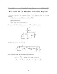
example: (lowpass) FIR filter, order n = 21impulse response h:0.20.1h(t)0−0.1−0.20 2 4 6 8 10 12 14 16 18 20tFilter design 4

• h is optimization variableChebychev designminimize max | H(ω) − H des (ω) |ω∈[0,π]• H des : R → C is (given) desired transfer function• convex problem• can add constraints, e.g., |h i | ≤ 1sample (discretize) frequency:minimize max |H(ω k ) − H des (ω k )|k=1,...,m• sample points 0 ≤ ω 1 < · · · < ω m ≤ π are fixed (e.g., ω k = kπ/m)• m ≫ n (common rule-of-thumb: m = 15n)• yields approximation (relaxation) of problem aboveFilter design 6

Chebychev design via SOCP:minimizesubject tot A (k) h − b (k) ≤ t,k = 1,...,mwhere 1 cos ωk cos(n−1)ωA (k) · · ·=k0 −sin ω k · · · −sin(n−1)ω kRHdes (ω k ) b (k) =IH des (ω k )⎡ ⎤h 0h = ⎣ . ⎦h n−1Filter design 7

Linear phase filterssuppose• n = 2N + 1 is odd• impulse response is symmetric about midpoint:h t = h n−1−t , t = 0, ...,n − 1then−iωH(ω) = h 0 + h 1 e−i(n−1)ω+ · · · + h n−1 e−iNω= e (2h 0 cos Nω + 2h 1 cos(N −1)ω + · · · + h N )Δ−iNω= e H(ω)Filter design 8

• term e −iNω represents N-sample delay• H (ω) is real• |H(ω)| = |H(ω)|• called linear phase filter ( H(ω) is linear except for jumps of ±π)Filter design 9

Lowpass filter specificationsδ 11/δ 1δ 2ω p ω s πidea:ω• pass frequencies in passband [0, ω p ]• block frequencies in stopband [ω s , π]Filter design 10

specifications:• maximum passband ripple (±20 log 10 δ 1 in dB):1/δ 1 ≤ |H(ω)| ≤ δ 1 , 0 ≤ ω ≤ ω p• minimum stopband attenuation (−20 log 10 δ 2 in dB):|H(ω)| ≤ δ 2 ,ω s ≤ ω ≤ πFilter design 11

Linear phase lowpass filter design• sample frequency• can assume wlog H (0) > 0, so ripple spec is1/δ 1 ≤ H(ω k ) ≤ δ 1design for maximum stopband attenuation:minimize δ 2subject to 1/δ 1 ≤ H(ω k ) ≤ δ 1 ,−δ 2 ≤ H(ω k ) ≤ δ 2 ,0 ≤ ω k ≤ ω pω s ≤ ω k ≤ πFilter design 12

• passband ripple δ 1 is given• an LP in variables h, δ 2• known (and used) since 1960’s• can add other constraints, e.g., |h i | ≤ αvariations and extensions:• fix δ 2 , minimize δ 1 (convex, but not LP)• fix δ 1 and δ 2 , minimize ω s (quasiconvex)• fix δ 1 and δ 2 , minimize order n (quasiconvex)Filter design 13

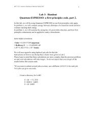
example• linear phase filter, n = 21• passband [0, 0.12π]; stopband [0.24π,π]• max ripple δ 1 = 1.012 (±0.1dB)• design for maximum stopband attenuationimpulse response h:0.20.1h(t)0−0.1−0.20 2 4 6 8 10 12 14 16 18 20tFilter design 14

frequency response magnitude (i.e., | H(ω) | ):110010|H(ω)|−110−21010−30 0.5 1 1.5 2 2.5 3ωfrequency response phase (i.e., H(ω)):321 H(ω)0−1−2−30 0.5 1 1.5 2 2.5 3ωFilter design 15

Equalizer designH(ω)G(ω)equalization: given• G (unequalized frequency response)• G des (desired frequency response)Δdesign (FIR equalizer) H so that G = GH ≈ G des• common choice: G des (ω) = e −iDω (delay)i.e., equalization is deconvolution (up to delay)• can add constraints on H, e.g., limits on |h i | or max ω |H(ω)|Filter design 16

Chebychev equalizer design:minimize maxω∈[0,π]convex; SOCP after sampling frequencyG(ω) − G des (ω) Filter design 17

time-domain equalization: optimize impulse response g˜ of equalizedsysteme.g., with G des (ω) = e −iDω ,g des (t) =1 t = D0 t = Dsample design:minimize max t =D | g˜(t) |subject to g˜(D) = 1• an LP• can useg˜(t) 2 ort=D t =D|g˜(t)|Filter design 18

extensions:• can impose (convex) constraints• can mix time- and frequency-domain specifications• can equalize multiple systems, i.e., choose H soG (k) H ≈ G des ,k = 1, ...,K• can equalize multi-input multi-output systems(i.e., G and H are matrices)• extends to multidimensional systems, e.g., image processingFilter design 19

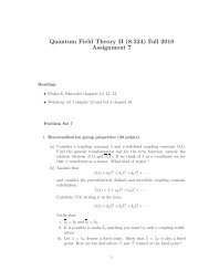
Equalizer design exampleunequalized system G is 10th order FIR:10.80.6g(t)0.40.20−0.2−0.40 1 2 3 4 5 6 7 8 9tFilter design 20

110 G(ω) |G(ω)|010−1100 0.5 1 1.5 2 2.5 3ω3210−1−2−30 0.5 1 1.5 2 2.5 3ωdesign 30th order FIR equalizer with G(ω) ≈ e −i10ωFilter design 21

Chebychev equalizer design:minimize max G(ω) ˜ − eequalized system impulse response g˜ω−i10ω10.8g˜(t)0.60.40.20−0.20 5 10 15 20 25 30 35tFilter design 22

equalized frequency response magnitude |G |110|Ge(ω)|010−1100 0.5 1 1.5 2 2.5 3ωequalized frequency response phase G 32 Ge(ω)10−1−2−30 0.5 1 1.5 2 2.5 3ωFilter design 23

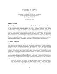
time-domain equalizer design:equalized system impulse response g˜minimize max | g˜(t) |t=1010.80.6g˜(t)0.40.20−0.20 5 10 15 20 25 30 35tFilter design 24

equalized frequency response magnitude |G |110|Ge(ω)|010−1100 0.5 1 1.5 2 2.5 3ωequalized frequency response phase G 321Ge(ω)0−1−2−30 0.5 1 1.5 2 2.5 3ωFilter design 25

Filter magnitude specificationstransfer function magnitude spec has formL(ω) ≤ |H(ω)| ≤ U(ω),ω ∈ [0,π]where L, U : R→R + are given• lower bound is not convex in filter coefficients h• arises in many applications, e.g., audio, spectrum shaping• can change variables to solve via convex optimizationFilter design 26

Autocorrelation coefficientsautocorrelation coefficients associated with impulse responseh = (h 0 ,...,h n−1 ) ∈ R n arer t = h τ h τ+tτ(we take h k = 0 for k < 0 or k ≥ n)• r t = r −t ; r t = 0 for |t| ≥ n• hence suffices to specify r = (r 0 , . ..,r n−1 ) ∈ R nFilter design 27

Fourier transform of autocorrelation coefficients isn−1−iωτR(ω) = e r τ = r 0 + 2r t cos ωt = | H(ω)|τ t=12• always have R(ω)≥0 for all ω• can express magnitude specification asL(ω) 2 ≤ R(ω) ≤ U(ω) 2 ,ω ∈ [0,π]. . . convex in rFilter design 28

Spectral factorizationquestion: when is r ∈ R n the autocorrelation coefficients of some h ∈ R n ?answer: (spectral factorization theorem) if and only if R(ω) ≥ 0 for all ω• spectral factorization condition is convex in r• many algorithms for spectral factorization, i.e., finding an h s.t.R(ω) = |H(ω)| 2magnitude design via autocorrelation coefficients:• use r as variable (instead of h)• add spectral factorization condition R(ω) ≥ 0 for all ω• optimize over r• use spectral factorization to recover hFilter design 29

choose h to minimizelog-Chebychev magnitude designmax | 20 log 10 | H(ω) | − 20 log 10 D(ω) |ω• D is desired transfer function magnitude(D(ω) > 0 for all ω)• find minimax logarithmic (dB) fitreformulate asminimize tsubject to D(ω) 2 /t ≤ R(ω) ≤ tD(ω) 2 ,0 ≤ ω ≤ π• convex in variables r, t• constraint includes spectral factorization conditionFilter design 30

example: 1/f (pink noise) filter (i.e., D(ω) = 1/ √ ω), n = 50,log-Chebychev design over 0.01π ≤ ω ≤ π1100102|H(ω)|−110−210−1 010 10ωoptimal fit: ±0.5dBFilter design 31

MIT OpenCourseWarehttp://ocw.mit.edu6.079 / 6.975 Introduction to Convex OptimizationFall 2009For information about citing these materials or our Terms of Use, visit: http://ocw.mit.edu/terms.