Bayesian Clustering with Regression - Facultad de Matemáticas ...

Bayesian Clustering with RegressionPeter MüllerUniversity of Texas M.D. Anderson Cancer Center, Houston, TX 77030, U.S.A.Fernando QuintanaDepartamento de Estadística, Pontificia Universidad Católica de Chile, Santiago,Chile.Gary RosnerUniversity of Texas M.D. Anderson Cancer Center, Houston, TX 77030, U.S.A.Summary. We consider clustering with regression, i.e., we develop a probabilitymodel for random partitions that is indexed by covariates. The motivating applicationis predicting time to progression for patients in a breast cancer trial. Weproceed by reporting a weighted average of the responses of clusters of earlierpatients. The weights should be determined by the similarity of the new patient’scovariate with the covariates of patients in each cluster. We achieve the desiredinference by defining a random partition model that includes a regression on covariates.Patients with similar covariates are a priori more likely to be clusteredtogether. Posterior predictive inference in this model formalizes the desired prediction.We build on product partition models (PPM). We define an extension of the PPMto include a regression on covariates by including in the cohesion function a newfactor that increases the probability of experimental units with similar covariatesto be included in the same cluster. We discuss implementations suitable for anycombination of continuous, categorical, count and ordinal covariates.

1. IntroductionWe develop a probability model for clustering with covariates, that is a probabilitymodel for partitioning a set of experimental units, where the probabilityof any particular partition is allowed to depend on covariates. The motivatingapplication is inference in a clinical trial. The outcome is time to progressionfor breast cancer patients. The covariates include treatment dose, initial tumorburden, an indicator for menopause and more. We wish to define a probabilitymodel for clustering patients with the specific feature that patients with equalor similar covariates should be more likely to co-cluster than others.Let i = 1, . . . , n, index experimental units, and let ρ n = {S 1 , . . . , S k } denotea partition of the n experimental units into k subsets S j . When n is obviousfrom the context we omit the subindex and write ρ. Let x i and y i denote thecovariates and response reported for the i-th unit. Let x n = (x 1 , . . . , x n ) andy n = (y 1 , . . . , y n ) denote the entire set of recorded covariates and data, and letx ∗ j = (x i, i ∈ S j ) and yj ∗ = (y i, i ∈ S j ) denote covariates and data correspondingto units in the j-th cluster. Sometimes it is convenient to introduceindicators e i ∈ {1, . . . , k} with e i = j if i ∈ S j , and use (k, e 1 , . . . , e n ) to describethe partition. We call a probability model p(ρ) a clustering model, excludingin particular purely constructive definitions of clustering as a specific algorithm(without reference to probability models). Many clustering models include, implicitlyor explicitly, a sampling model p(y | ρ). Probability models for p(ρ)and inference for clustering have been extensively discussed over the past fewyears. See Quintana (2006) for a recent review. In this paper we are interestedin adding a regression to replace p(ρ) with p(ρ | x).We focus on the product partition models (PPM). The PPM (Hartigan, 1990;Barry and Hartigan, 1993) constructs p(ρ) by introducing cohesion functionsc(A) ≥ 0 for A ⊂ {1, . . . , n} that measure how tightly grouped the elements in2

A are thought to be, and defines a probability model for a partition ρ and datay asp(ρ) ∝ ∏ k∏c(S i ) and p(y | ρ) = p j (y Sj ). (1)j=1Model (1) is conjugate. The posterior p(ρ | y) is again in the same product form.Alternatively, the species sampling model (SSM) (Pitman, 1996; Ishwaranand James, 2003) defines an exchangeable probability model p(ρ) that dependson ρ only indirectly through the cardinality of the partitioning subsets, p(ρ) =p(|S 1 |, . . . , |S k |). The SSM can be alternatively characterized by a sequence ofpredictive probability functions (PPF) that describe how individuals are sequentiallyassigned to either already formed clusters or to start new ones. The choiceof the PPF is not arbitrary. One has to make sure that a sequence of randomvariables that are sampled by iteratively applying the PPF is exchangeable. Thepopular Dirichlet process (DP) model (Ferguson, 1973; Antoniak, 1974) is a specialcase of a SSM. Moreover, the marginal distribution that a DP induces onpartitions is also a PPM with cohesions c(A) = M × (|A| − 1)! (Quintana andIglesias, 2003; Dahl, 2003). Here M denotes the total mass parameter of the DPprior.Model based clustering (Banfield and Raftery, 1993; Dasgupta and Raftery,1998; Fraley and Raftery, 2002) implicitly defines a probability model on clusteringby assuming a mixture modelk∑p(y i | η, k) = τ j p j (y i | θ j ),j=1where η = (θ 1 , . . . , θ k , τ 1 , . . . , τ k ) are the parameters of a size k mixture model.Together with a prior p(k) on k and p(θ, τ | k), the mixture defines a probabilitymodel on clustering. Consider the equivalent hierarchical modelp(y i | e i = j, k, η) = p j (y i | θ j ) and P r(e i = j | k, η) = τ j . (2)3

The implied posterior distribution on (e 1 , . . . , e n ) and k defines a probabilitymodel on ρ n . Richardson and Green (1997) develop posterior simulation strategiesfor mixture of normal models. Green and Richardson (1999) discuss therelationship to DP mixture models.Especially in the context of spatial data, a popular clustering model is basedon Voronoi tessellations (Green and Sibson, 1978; Okabe et al., 2000; Kim et al.,2005). For a review see, for example, Denison et al. (2002). Although notusually considered as a probability model on clustering, it can be defined assuch by means of the following construction. We include it in this brief review ofclustering models because of its similarity to the model proposed in this paper.Assume x i are spatial coordinates for observation i. Let d(x 1 , x 2 ) denote adistance measure, for example Euclidean distance in R 2 . Clusters are definedwith latent cluster centers T j , j = 1, . . . , k, by setting e i = arg min j d(x i , T j ).That is, a partition is defined by allocating each observation to the cluster whosecenter T j is closest to x i . Conditional on T , cluster allocation is deterministic.Marginalizing with respect to a prior on T we could define a probability modelp(ρ | k).In this paper we build on the PPM (1) to define a covariate-dependent randompartition model by augmenting the PPM with an additional factor that inducesthe desired dependence on the covariates. We refer to the additional factoras similarity function. Focusing on continuous covariates a similar approach isbeing proposed in independent current work by Park and Dunson (2007). Shahbabaand Neal (2007) introduce a related model for categorical outcomes, i.e.,classification. They use a logistic regression for the categorical outcome on covariatesand a random partition of the samples, with cluster-specific regressionparameters in each partitioning subset. The random partition is defined by aDP prior and includes the covariates as part of the response vector.4

In section 2 we state the proposed model and considerations in choosingthe similarity function. In section 3 we show that the computational effort ofposterior simulation remains essentially unchanged from PPM models withoutcovariates. In 4 we propose specific choices of the similarity function for commondata formats. In section 5 we show a simulation study and a data analysisexample. In the context of the simulation study we contrast the proposed approachto an often used ad-hoc implementation of including the covariates in anaugmented response vector.2. Clustering with CovariatesWe build on the PPM (1), modifying the cohesion function c(S j ) with an additionalfactor that achieves the desired regression. Recall that x ∗ j = (x i, i ∈ S j )denotes all covariates for units in the j-th cluster.Let g(x ∗ j ) denote a nonnegativefunction of x ∗ jthat formalizes similarity of the x i with larger valuesg(x ∗ j ) for sets of covariates that are judged to be similar. We define the modelp(ρ | x) ∝k∏g(x ∗ j ) · c(S j ) (3)with the normalization constant g n (x n ) = ∑ ρ n∏ kj=1 g(x∗ j )c(S j).j=1By a slightabuse of notation we include x behind the conditioning bar even when x is not arandom variable. We will later discuss specific choices for the similarity functiong. As a default choice we propose to define g(·) as the marginal probability inan auxiliary probability model q, even if x i are not considered random,∫g(x ⋆ j ) ≡∏i∈S jq(x i | ξ j ) q(ξ j )dξ j . (4)The function (4) satisfies the following two properties that are desirable for a similarityfunction in (3). First, we require symmetry with respect to permutationsof the sample indices i. The probability model must not depend on the order5

x n , x n+1 ):p(ρ n | x n ) = ∑ e n+1∫p(ρ n+1 | x n , x n+1 ) q(x n+1 | x n ) dx n+1 , (5)for the probability model q(x n+1 | x n ) ∝ g n+1 (x n+1 )/g n (x n ).We complete the random partition model (3) with a sampling model thatdefines independence across clusters and exchangeability within each cluster.We include cluster-specific parameters θ j and common hyperparameters η:k∏ ∏p(y n | ρ n , θ, η, x n ) =p(θ j | η).j=1i∈S jp(y i | x i , θ j , η) and p(θ | η) = ∏ jThe resulting model extends PPMs of the type (1) while keeping the productstructure.(6)3. Posterior InferenceA practical advantage of the proposed default choice for g(x ∗ j ) is that it greatlysimplifies posterior simulation. In words, posterior inference in (3) and (6) isidentical to the posterior inference that we would obtain if x i were part of therandom response vector y i . Formally, define an auxiliary model q(·) by replacing(6) withq(y n , x n | ρ n , θ, η) = ∏ j∏i∈S jp(y i | x i , θ j , η) q(x i | ξ j ) and q(θ, ξ | η) = ∏ jp(θ j | η)q(ξ j )and replace the covariate-dependent prior p(ρ n | x n ) by the PPM q(ρ n ) ∝∏ c(Sj ). We continue to use q(·) for the auxiliary probability model that isintroduced as a computational device only, and p(·) for the proposed inferencemodel.The posterior distribution q(ρ | y n , x n ) under the auxiliary model isidentical to p(ρ | y n , x n ) under the proposed model. An important caveat is that(7)7

ξ j and θ j must be a priori independent. In particular the prior on θ j and q(ξ j )must not include common hyperparameters. If we had p(θ j | η) and q(ξ j | η) dependon a common hyperparameter η, then the posterior distribution under theauxiliary model (7) would differ from the posterior under the original model. Letq(x n | η) = ∑ ρ n∏j q(x⋆ j | ξ j)q(ξ j | η). The two posterior distributions woulddiffer by a factor 1/q(x n | η). The implication on the desired inference can besubstantial. See the results in section 5 for an example and more discussion.However, the restriction that θ j and ξ j be independent is natural. The functiong(x ∗ j ) defines similarity of the experimental units in one cluster and is chosen bythe user. There is no notion of learning about the similarity.A minor complication arises with posterior predictive inference, i.e., reportingp(y n+1 | x n , x n+1 ). Using ˜x = x n+1 , ỹ = y n+1 and ẽ = e n+1 to simplify notation,we find p(ỹ | ˜x, x n , y n ) = ∫ p(ỹ | ˜x, ρ n+1 , y n ) dp(ρ n+1 | ˜x, y n , x n ). The integral issimply a sum over all configurations ρ n+1 . But it is not immediately recognizableas a posterior integral with respect to p(ρ n | y n ). This can easily be overcomeby an importance sampling reweighting step. The prior on ρ n+1 = (ρ n , ẽ) canbe written asp(ẽ = l, ρ n | ˜x, x n ) ∝ ∏ j≠lc(S j )g(x ∗ j ) c(S l ∪ {n + 1})g(x ∗ l , ˜x) =p(ρ n | x n ) g(x∗ l , ˜x)g(x ∗ l ) .c(S l ∪ {n + 1})c(S l )Let q l (˜x | x ∗ l ) ≡ g(x∗ l , ˜x)/g(x∗ l). The posterior predictive distribution becomesp(ỹ | ˜x, y n , x n ) ∝∫ kn+1∑l=1p(ỹ | y ∗ l , ẽ = l) q l (˜x | x ∗ l ) c(S l ∪ {n + 1})c(S l )p(ρ n | y n , x n ) dρ n .Therefore, sampling from (8) is implemented on top of posterior simulation forρ n ∼ p(ρ n | y n ). For each imputed ρ n , generate ẽ = l with probabilities propor-(8)8

tional tow l = q l (˜x | x ∗ l ) c(S l ∪ {n + 1})c(S l )and generate ỹ from p(ỹ | yl ∗, ẽ = l), weighted with w l, noting that in the specialcase l = k n + 1 we get w kn+1 = g(x ∗ )c({n + 1}).Reporting posterior inference for random partition models is complicated byproblems related to the label switching problem. See Jasra et al. (2005) for arecent summary and review of the literature. Usually the focus of inference insemiparametric mixture models like (6) is on density estimation and prediction,rather than inference for specific clusters and parameter estimation. Predictiveinference is not subject to the label switching problem, as the posterior predictivedistribution marginalizes over all possible partitions. However, in some exampleswe want to highlight the choice of the clusters. We briefly comment on theimplementation of such inference. We use an approach that we found particularlymeaningful to report inference about the regression p(ρ | x). We report inferencestratified by k, the number of clusters. For given k we first find a set of kindices I = (i 1 , . . . , i k ) with high posterior probability of the correspondingcluster indicators being distinct, i.e., P r(D I | y) is high for D I = {e i ≠ e j for i ≠j and i, j ∈ I}. To avoid computational complications, we do not insist onfinding the k-tuple with the highest posterior probability. We then use i 1 , . . . , i kas anchors to define cluster labels by restricting posterior simulations to k clusterswith the units i j in distinct clusters. Post-processing MCMC output, this iseasily done by discarding all imputed parameter vectors that do not satisfy theconstraint. We re-label clusters, indexing the cluster that contains unit i j ascluster j. Now it is meaningful to report posterior inference on specific clusters.The proposed post-processing is similar to the pivotal reordering suggested inMarin and Robert (2007, chapter 6.4). An alternative loss function based methodto formalize inference on partitions is discussed in Lau and Green (2007).9

4. Similarity FunctionsFor continuous covariates we suggest as a default choice for g(x ∗ j ) the marginaldistribution of x ∗ junder a normal sampling model. Let N(x; m, V ) denotea normal model for the random variable x, with moments m and V , and letGa(x; a, b) denote a Gamma distributed random variable with mean a/b. Weuse q(x ∗ j | ξ j) = ∏ i∈S jN(x i ; m j , s j ), with a conjugate prior for ξ j = (m j , s j )as p(ξ j ) = N(m j ; m, B) · Ga(s −1j ; ν, S 0 ), with fixed m, B, ν, S 0 . The mainreason for this choice is operational simplicity. A simplified version uses fixeds j ≡ s. The resulting function g(x ⋆ j ) is the joint density of a collection ofcorrelated multivariate normal vectors, with mean m and Cor(x i , x i ′) = B/(V +B). The fixed variance s specifies how strong we weigh similarity of the x. Inimplementations we used s = c 1 Ŝ, wherecovariate, and c 1Ŝ is the empirical variance of the= 0.5 is a scaling factor that specifies over what range weconsider values of this covariate as similar. Analogously we set B = c 2 Ŝ withc 2 = 10. The choice between fixed s versus variable s j should reflect priorjudgement on the variability of clusters. Variable s j allows for some clusters toinclude a wider range of x values than others.When constructing a cohesion function for categorical covariates, a defaultchoice is based on a Dirichlet prior. Assume x i is a categorical covariate, x i ∈{1, . . . , C}. To define g(x ∗ j ), let q(x i = c) = ξ jc denote the probability massfunction. Together with a conjugate Dirichlet prior, q(ξ j ) = Dir(α 1 , . . . , α C ) wedefine the similarity function as a Dirichlet-categorical probability∫g(x ∗ j ) =∏∫ξ j,xi dq(ξ j ) =i∈S jC∏c=1ξ njcjc dq(ξ j ), (9)with n jc = ∑ i∈S jI(x i = c). This is a Dirichlet-multinomial model without themultinomial coefficient. For binary covariates the similarity function becomes aBeta-Binomial probability without the Binomial coefficient. The choice of the10

hyperparameters α needs some care. To facilitate the formation of clusters thatare characterized by the categorical covariates we recommend Dirichlet hyperparametersα c < 1. For example, for C = 2, the bimodal nature of a Betadistribution with such parameters assigns high probability to binomial successprobabilities ξ j1 close to 0 or 1. Similarly, the Dirichlet distribution with parametersα c < 1 favors clusters corresponding to specific levels of the covariate.model.A convenient specification of g(·) for ordinal covariates is an ordinal probitThe model can be defined by means of latent variables and cutoffs.Assume an ordinal covariate x with C categories. Following Johnson and Albert(1999), consider a latent trait Z and cutoffs −∞ = γ 0 < γ 1 ≤ γ 2 ≤ · · · ≤γ C−1 < γ C = ∞, so that x = c if and only if γ c−1 < Z ≤ γ c . Consider fixedcutoff values γ c = c − 1, c = 1, . . . , C − 1, and a normally distributed latenttrait, Z i ∼ N(m j , s j ). Let Φ c = Pr(γ c−1 < Z ≤ γ c | m j , s j ) denote the normalquantiles. We define q(x i | s i = j, m j , s j ) = Φ c . The definition of the similarityfunction is completed with q(m j , s j ) as a normal-inverse gamma distribution asfor the continuous covariates. We have∫∏ Cq(x ∗ j ) =c=1Φ ncjcwhere n cj = ∑ i∈S jI{x i = c}.N(m j ; m, B) Ga(s −1j ; ν, S 0 ) dm j ds j ,Finally, to define g(·) for count-type covariates, we use a mixture of Poissondistributions∫g(x ∗ 1j ) = ∏i∈S jx i !Pi∈S x iξjj exp(−ξ j |S j |) dq(ξ j ). (10)With a conjugate gamma prior, q(ξ j ) = Ga(ξ j ; a, b), the similarity function g(x ∗ j )allows easy analytic evaluation. As a default, we suggest choosing a = 1 anda/b =cŜ, where Ŝ is the empirical variance of the covariate, and a/b is theexpectation of the gamma prior.The main advantage of the proposed similarity functions is computational11

simplicity of posterior inference. A minor limitation is the fact that the proposeddefault similarity functions, in addition to the desired dependence of therandom partition model on covariates also include a dependence on the clustersize n j = |S j |. From a modeling perspective this is undesirable. The mechanismto define size dependence should be the underlying PPM and the cohesion functionsc(S j ) in (3). However, we argue that the additional cluster size penaltythat is introduced through g(·) can be ignored in comparison to, for example,the cohesion function c(S j ) = M(n j − 1)! that is implied by the popular DPprior.Proposition 2:penalty in model (3).The similarity function introduces an additional cluster sizeConsider the case of constant covariates, x i ≡ x, andlet n j denote the size of cluster j. The default choices of g(x ⋆ j ) for continuous,categorical and count covariates introduce a penalty for large n j , withlim nj→∞ g(x ⋆ j ) = 0. But the rate of decrease is ignorable compared to the cohesionc(S j ). Let f(n j ) be such that lim nj→∞ g(x ⋆ j )/f(n j) ≥ M with 0 < M < ∞.For continuous covariates the rate is f(n j ) = (2π) − n j2 V − n j −12 (ρ+n j ) 1 2 with ρ =V/B. For categorical covariates it is f(n j ) = (A + n j ) A−αx , with A = ∑ c α c.For count covariates it is f(n j ) = C − n j2 (α + n j x) 1 2 with C = 2πx exp(1/6x).Proof: see appendix. ✷Another important concern besides the dependence of g(·) on n j is the dependenceon q(ξ j ) in the auxiliary model in (4). In particular, we focus on thedependence on possibly hyperparamters φ that index q(ξ j ). We write q(ξ j | φ)when we want to highlight the use of such (fixed) hyperparameters. The auxiliarymodels q(·) for all proposed default similarity functions include such hyperpa-12

ameters. Model (3) and (4) implies conditional cluster membership probabilitiesp(e n+1 = j | x n+1 , x n , ρ n ) ∝ c(S j ∪ {n + 1})c(S j )g(x ⋆ j , x n+1)g(x ⋆ j} {{ ) (11)}≡q j(x n+1|x ⋆ j ,φ)j = 1, . . . , k n , with the convention g(∅) = c(∅) = 1. The cluster membershipprobabilities (11) are asymptotically independent of φ. Noting that q j (x n+1 |x ⋆ j , φ) can be written as a posterior predictive distribution in the auxiliary model,the statement follows from the asymptotic agreement of posterior predictivedistributions.Proposition 3:Consider any two similarity functions g h (x ⋆ j ), h = 1, 2, basedon an auxiliary model (4) with different probability models q h (ξ j ), s = 1, 2,but the same model q(x i | ξ j ). For example, q h (ξ j ) = q(ξ j | φ h ). Assumethat both auxiliary models satisfy the regularity conditions of Schervish (1995,Section 7.4.2) and assume q(x i | ξ) ≤ K is bounded. Let q h j (x n+1 | x ⋆ j ) denotethe un-normalized cluster membership probability in equation (11) under q h (ξ j ).Thenlimn q1 j (x n+1 | x ⋆ j ) − qj 2 (x n+1 | x ⋆ j ) = 0 (12)j→∞The limit is a.s. under i.i.d. sampling from q(x i | ξ 0 ).See the appendix for a straightforward proof making use of asymptotic posteriornormality only. The statement is about asymptotic cluster membershipprobabilities for a future unit only and should not be overinterpreted.marginal probability for a set of elements forming a cluster does depend onhyperparameters.proposition 2.TheAn example are the expressions for g(x ⋆ j ) in the proof of13

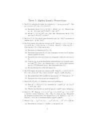
Y0 1 20 5 10 15 20 25TY−0.5 0.0 0.5 1.0 1.534567●●●●●●●●●●●●●●●●●0 5 10 15 20 25 30T●●●●●●●●●34567datatrue mean responseFig. 1. Simulation example. Data (left panel) and simulation truth for the mean responseE(y i | x i) as a function of the covariate x i (right panel).5. Examples5.1. Simulation StudyWe set up a simulation study with a 6-dimensional response y i , and a continuouscovariate x i , and for n = 47 data points (y i , x i ), i = 1, . . . , n. The simulationis set up to mimic responses of blood counts over time for patients undergoingchemo-immunotherapy. Each data point corresponds to one patient. The sixresponses for each patient could be for six key time points over the course of onecycle of the therapy. The covariate is a treatment dose. In the simulation studywe sampled x i from 5 possible values, x i ∈ {3, 4, 5, 6, 7}. For each value of x wedefined a different mean vector. Figure 1b shows the 5 distinct mean vectors forthe 6-dimensional response (plotted against days T ). The bullets indicate thesix responses. Adding a 6-dimensional normal residual we generated the datashown in Figure 1a.We then implemented the proposed model for covariate-dependent clustering14

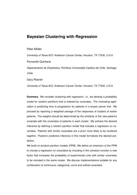
to define a random partition model with a regression on the covariate x i , asproposed earlier. Let N(x; m, s) indicate a normal distribution for the randomvariable x, with moments (m, s), let W (V ; ν, S) denote Wishart prior for a randommatrix V with scalar parameter ν and matrix variate parameter S, and letGa(s; a, b) denote a gamma distribution parameterized to have mean a/b. Letθ j = (µ j , V j ). We used a multivariate normal model p(y i | θ j ) = N(µ j , V j ), witha conditionally conjugate prior for θ j , i.e., p(θ j ) = N(µ j ; m y , B y ) W (V −1j ; s, Sy −1 ).The model is completed with conjugate hyperpriors for m y , B y and S y . The similarityfunction is a normal kernel. We use∫ ∏g(x ⋆ j ) = N(x i ; m j , s j ) N(m j ; m, B) Ga(s −1j ; ν, S 0 ).i∈S jThe hyperparameters m, B, S 0 are fixed.Figure 2 summarizes posterior inference by the posterior predictive distributionfor y n+1 arranged by x n+1 . The marginal posterior distribution forthe number of clusters assigns posterior probabilities p(k = 3 | data) = 76%,p(k = 4 | data) = 20% and p(k = 5 | data) = 3%.We used the proceduredescribed at the end of section 3 to report cluster-specific summaries. Conditionalon k = 3, the three clusters are characterized by x i = 3.4(0.2) for thefirst cluster, x i = 5(0) for the 2nd cluster and x i = 7(0) for the third cluster(posterior means and standard deviations of x i assigned to each cluster). Theaverage cluster sizes are 24, 11 and 11.For comparison, the right panel of the same figure shows posterior predictiveinference in a model using a PPM prior on clustering, without the use of covariates.In this case, the inference is by construction the same for all covariatevalues.A technically convenient ad-hoc solution to include covariates in a samplingmodel is to proceed as if the covariates were part of the response vector. Thisapproach is used, for example in Mallet et al. (1988) or Müller et al. (2004).15

E(Z | dta)−0.5 0.0 0.5 1.0 1.53●4●5●6●7●●●●●x34567●●●●●●●●0 5 10 15 20 25 30TIME●●●●●●●●● 5● 34● 6● 7E(Z | dta)−0.5 0.0 0.5 1.0 1.5●●●●●●0 5 10 15 20 25 30TIMEFig. 2. Simulation example. Estimated mean response under the proposed covariateregression (left panel) and without (right panel).Doing so introduces an additional factor in the likelihood.Let y genericallydenote the response, x the covariate, and θ the model parameters. Treating thecovariate as part of the response vector is equivalent to replacing the samplingmodel p(y | x, θ) by p(y | x, θ) · p(x | θ). Equivalently, one can interpret theadditional factor p(x | θ) as part of the prior. The reported posterior inference isas if we had changed the prior model from the original p(θ) to ˜p(θ) ∝ p(θ)p(x | θ).Wong et al. (2003) use this interpretation for a similar construction in the contextof prior probability models for a positive definite matrix.The implied modification of the prior probability model could be less innocuousthan what it seems. We implemented inference under the PPM prior model(1), without covariates, and a sampling model as before, but now for an extendedresponse vector augmented by the covariate x i . We assume a multivariate normalsampling model p(y i , x i | θ j ) = N(µ j , V j ), with a conditionally conjugateprior for θ j , i.e., p(θ j ) = N(µ j ; m y , B y ) W (V −1j; s, Sy−1 ). As before the model iscompleted with conjugate hyperpriors for m y , B y and S y . The hyperparameters16

●●●●●E(Z | dta)0.0 0.5 1.03●4●5●6●7●●●x34567●●●●●●●●●●●● 3● 4● 5● 6● 7●●0 5 10 15 20 25 30TIMEFig. 3. Prediction for ỹ arranged by ˜x for the covariate response model with the additionalfactors p(x n j | θ j, η) in the prior (left panel). Posterior distribution on the size of thelargest cluster under the covariate response model (right panel). The example has atotal sample size of n = 47.are chosen exactly as before. The additional 7-th row and column of the priormeans for B y and S y are all zero except for the (7,7) diagonal element whichwe fix at E(m j ) and E(s j ) to match the moments in the auxiliary model q(·)from before. We refer to the model as covariate response model, in contrast tothe proposed covariate regression model. Figure 3 shows inference under thismodified model which differs from the proposed model by the additional factorsp(x n j | θ j ) in the prior. In this example, the covariate response model leadsto a much reduced size of the partition. With posterior probability 97% thepartition includes only one cluster. This in turn leads to essentially a simplelinear regression implied by the dominating multivariate normal p(x i , y i | θ 1 ),as clearly seen in Figure 3. In contrast, under the proposed covariate regressionmodel the size of the largest cluster is estimated between 16 and 26 (not shown).The covariate response model could be modified to better match the simulation17

truth. This could be achieved, for example, by fixing the hyperparameters ina way that avoids correlation of the first 6 and the last dimension of µ j . Theresulting model would have exactly the format of (3).We thus do not consider the principled way of introducing the covariatesin the PPM to be the main feature of the proposed model. Rather, we arguethat the proposed model greatly simplifies the inclusion of covariates includinga variety of data formats. It would be unnecessarily difficult to attempt the constructionof a joint model for continuous responses and categorical, binary andcontinuous covariates. We argue that it is far easier to focus on a modificationof the cohesion function and that this does not imply restricting the scope of theproposed models. This is illustrated in the following data analysis example.5.2. A Survival Model with Patient Baseline CovariatesWe consider data from a high-dose chemotherapy treatment of women withbreast cancer. The data for this particular study have been discussed in Rosner(2005) and come from Cancer and Leukemia Group B (CALGB) Study 9082.It consists of measurements taken from 763 randomized patients, available asof October 1998 (enrollment had occurred between January 1991 to May 1998).The response of interest is the survival time, defined as the time until death fromany cause, relapse, or diagnosis with a second malignancy. There are two treatments,one involving a low dose of the anticancer drugs, and the other consistingof aggressively high dose chemotherapy. The high-dose patients were given considerableregenerative blood-cell supportive care (including marrow transplantation)to help decreasing the impact of opportunistic infections rising from theseverely-affected immune system. The number of observed failures was 361, with176 under high dose and 185 under low dose chemotherapy.The dataset also includes information on the following covariates for each18

patient: a treatment indicator defined as 1 if a high-dose was administered and0 otherwise (HI); age in years at baseline (AGE); the number of positive lymphnodes found at diagnosis (POS) (the more the worse the prognosis, i.e. the morelikely the cancer has spread); tumor size in millimeters (TS), a one-dimensionalmeasurement; an indicator of whether the tumor is positive for the estrogenor progesterone receptor (ER+) (patients who were positive also received thedrug tamoxifen and are expected to have better risk) and an indicator of thewoman’s menopausal status, defined as 1 if she is either perimenopausal or postmenopausalor 0 otherwise (MENO). Two of these six covariates are continuous(AGE,TS), three are binary (ER+,MENO,HI) and one is a count (POS).First we carried out inference in a model using the indicator for high-doseas the only covariate, i.e, x i = HI. We implemented model (6) with a similarityfunction for the binary covariate based on the beta-binomial model (9).used α = (0.1, 0.1) to favor clusters with homogenous dose assignment. Conditionalon an assumed partition ρ n we use a normal sampling model p(y i |θ j ) = N(µ j , V j ), with a conjugate normal-inverse gamma prior p(θ j | η) =N(µ j | m y , B y ) Ga(V −1jWe| s/2, sS y /2) and hyperprior m y ∼ N(a m , A m ), S y ∼Ga(q, q/R). Here η = (a m , A m , B y , q, R) are fixed hyperparameters. We usea m = ̂m, the sample average of y i , A m = 100, B y = 100 2 ,s = q = 4, andR = 100. Figure 4a shows inference summaries.The posterior distributionp(k | data) for the number of clusters is shown in Figure 5. The three largestclusters contain 28%, 23%, and 14% of the experimental units.Next we extended the covariate vector to include all six covariates. Denoteby x i = (x i1 , . . . , x i6 ) the 6-dimensional covariate vector. We implement randomclustering with regression on covariates as in model (6). The similarity functionis defined as6∏g(x ∗ j ) = g l (x ∗ jl). (13)l=119

S0.3 0.4 0.5 0.6 0.7 0.8 0.9 1.0LOHIHAZARD0.000 0.005 0.010 0.015 0.020a=10.3 0.4 0.5 0.6 0.7 0.8 0.9 1.0LOHI0 20 40 60 80 100 120DAYS0 20 40 60 80 100 120MONTHS0 20 40 60 80 100 120 140S(t) ≡ p(y n+1 ≥ t | data) hazard h(t) data (KM)Fig. 4. Survival example: Estimated survival function (left panel) and hazard (centerpanel), arranged by x ∈ {HI, LO}. The grey shades show pointwise one posterior predictivestandard deviation uncertainty. The right panel shows the data for comparison(Kaplan-Meier curve by dose).p(k | data)0.00 0.02 0.04 0.06 0.08% HI DOSE0 20 40 60 80 100●●●●●●5 10 15 20 25 30 35k0 20 40 60 80 100 120PFSp(k | data)Proportion high dose and mean PFSFig. 5. Survival example: Posterior for the number of clusters k (left panel), andproportion of patients with high dose (%HI) and average progression free survival (PFS)by cluster. The size (area) of the bullets is proportional to the average cluster size.20

For each covariate we follow the suggestion in Section 4 to define a factor g l (·) ofthe similarity function, using hyperparameters specified as follows. The similarityfunction for the three binary covariates is defined as in (9) with α o = (0.1, 0.1)for HI, and α o = (0.5, 0.5) for ER+, and MENO. The two continuous covariatesAGE and TS were standardized to sample mean 0 and unit standard deviation.The similarity functions were specified as described in section 4, withfixed s = 0.25, m = 0 and B = 1. Finally, for the count covariate POS weused the similarity function (10) with (a, b) = (1.5, 0.1). The sampling model isunchanged from before.We assume that censoring times are independent of the event times andall parameters in the model. Posterior predictive survival curves for variouscovariate combinations are shown in Figure 6. In the figure, “baseline” refers toHI = 0, tumor size 38mm (the empirical median), ER = 0, Meno = 0, averageage (44 years), and POS = 15 (empirical mean). Other survival curves arelabeled to indicate how the covariates change from baseline, with TS− indicatingtumor size 26mm (the empirical first quartile), TS+ indicating tumor size 50mm(third quartile), HI referring to high-dose chemotherapy, and ER+ indicatingpositive estrogen or progesterone receptor status. The inference suggests thattreated patients with tumor size below the empirical median and that werepositive for estrogen or progesterone receptor have almost uniformly highestpredicted survival curves than any other combination of covariates.Figure 7 summarizes features of the posterior clustering. Interestingly, clustersare typically highly correlated to the postmenopausal status, as seen in theright panel. The high-dose indicator is also seen to be positively correlated tothe progression-free survival (PFS).The model used so far consisted of a mixture of normal sampling model forthe event times y i . A more parsimonious sampling model is proposed in Rosner21

S0.2 0.4 0.6 0.8 1.0TS− HI ER+TS+ HI ER+HI ER+TS− HITS−HITS− ER+(baseline)ER+TS+ ER+0 20 40 60 80 100 120MONTHSS(t | x)Fig. 6. Survival example: Posterior predictive survival function S(t | x) ≡ p(y n+1 ≥t | x n+1 = x, data), arranged by x. The “baseline” case refers to all continuous andcount covariates equal to the empirical mean, and all binary covariates equal 0. Thelegend indicates TS− and TS+ for tumor size equal 26mm and 50mm (first and thirdempirical quartile), HI for HI = 1 and ER+ for ER = 1. The legend is sorted by thesurvival probability at 5 years, indicated by a thin vertical line..22

p(k | data)0.00 0.02 0.04 0.06 0.08 0.10 0.1220 25 30 35 40k% HI DOSE0 20 40 60 80 100● ●●●●●●0 20 40 60 80 100 120PFS% Meno0 20 40 60 80 100●●●●0 20 40 60 80 100 120PFS●p(k | data) PFS and % high dose PFS and % postmenopausalFig. 7. Survival example: Posterior distribution for the number of clusters (left panel),mean PFS and % high dose patients per cluster (center panel), mean PFS and %postmenopausal patients per cluster (right panel).S0.2 0.4 0.6 0.8 1.0TS− HI ER+ER+TS− ER+HI ER+TS− HITS−TS+ HI ER+HI(baseline)TS+ ER+0 20 40 60 80 100 120 140MONTHSFig. 8. Survival example with the piecewise exponential sampling model: estimatedsurvival S(t | x) arranged by covariates x.23

(2005) who uses a piece-wise exponential sampling model with survival functionP r(y ≥ t) =⎧⎪⎨S(t | λ 1 , λ 2 , λ 3 , τ 1 , τ 2 ) =⎪⎩e −λ1t if t ≤ τ 1 ,e −λ1τ1 e −λ2(t−τ1) if τ 1 < t ≤ τ 2 ,e −λ1τ1 e −λ2(τ2−τ1) e −λ3(t−τ2) if τ 2 < t,(14)where λ = (λ 1 , λ 2 , λ 3 ) defines the exponential rates for each piece, and thechange-points τ 1 and τ 2 are fixed as 1 and 2 years, respectively.Inference under sampling model (14) is summarized in Figure 8. The posteriordistribution on the number of clusters (not shown) now shows a posteriormode for k = 7, and positive posterior probability for 4 ≤ k ≤ 14. The averagecluster sizes of the 3 largest clusters are 43%, 30% and 18% of all observations.Compare with Figure 7a. The simple normal sampling model underlying theinference in Figure 7 requires larger size mixtures than the more parsimoniousmodel (14). On the other hand the fixed change-points τ 1 and τ 2 lead to discontinuitiesin the densities that are visible as the corners in the estimated survivalfunctions in Figure 8. The terms in the mixture are models of the form (14).Each mixture term is a distribution with support over the entire real line. Thisis in contrast to the mixture of normal kernels with more localized support. 6.6. ConclusionWe have proposed a novel model for random partitions with a regression oncovariates. The model builds on the popular PPM random partition models byintroducing an additional factor to modify the cohesion function. We refer to theadditional factor as similarity function. It increases the prior probability thatexperimental units with similar covariates are co-clustered. We provide defaultchoices of the similarity function for popular data formats.The main features of the model are the possibility to include additional prior24

information related to the covariates, the principled nature of the model construction,and a computationally efficient implementation. We compared themodel with a popular ad-hoc implementation that includes the covariates aspart of an augmented response vector. This approach is feasible in particularwhen both, the response variable y i and the covariate x i are continuous. Ajoint multivariate normal model for the augmented response vector implicitlyintroduces the desired regression on covariates. Besides issues of appropriatelikelihood specification, the main limitation of such an approach is the practicalrestriction to continuous responses and covariates. Building a joint model forother data formats is possible, but would be more complicated than a straightforwardprincipled approach that treats x i as covariates.Among the limitations of the proposed method is an implicit penalty forthe cluster size that is implied by the similarity function. Consider all equalcovariates x i ≡ x. The value of the similarity functions proposed in section 4decreases across cluster size. This limitation could be mitigated by allowing anadditional factor c ⋆ (|S j |) in (6) to compensate the size penalty implicit in thesimilarity function.The programs are available as a function in the R package clusterX athttp://odin.mdacc.tmc.edu/∼pm/prog.html The function clusterx(.) implementsthe proposed covariate dependent random partition model for an arbitrarycombination of continuous, categorical, binary and count covariates, usinga mixture of normal sampling model for y i .AcknowledgmentResearch was partially supported by NIH under grant 1R01CA75981, by FONDE-CYT under grant 1060729 and the Laboratorio de Análisis Estocástico PBCT-ACT13. Most of the research was done while the first author was visiting at25

Pontificia Universidad Católica de Chile.AppendixProof of Proposition 2For simplicity we drop the j index in n j , x ⋆ j etc., relying on the context to preventambiguity. Let 1 denote a (n × 1) vector of all ones. For continuous covariates,evaluation of the g(x ⋆ ) gives{g(x ⋆ ) = (2π) − n 2 [(V + nB)V n−1 ] − 1 2 exp − 1 2 (x − 1 ) }B(I m)2 V 1′ − J 1V + nBwhich after some further simplification becomes(2πV n−1n) − n2(ρ + n) 1 2 M(n)with lim n→∞ M(n) = M, 0 < M < ∞. For categorical covariates, Stirling’sapproximation and some further simplifications givesg(x ⋆ ) = ∏ Γ(A)∏ Γ(αc ) Γ(αx+n)Γ(α x) 1≥M(n).Γ(αcA−αx) Γ(A + n) A + nSimilarly, for count covariates we find( n 1g(x ⋆ b) =x!) a Γ(a) + nxΓ(a) (b + n) a+nx ≥ (2πx)− n 2 e− n112x (α + nx) 2 · M(n).Proof of Proposition 3The ratio g h (x ⋆ j , x n+1)/g h (x ⋆ j ) defines the conditional probability qh j (x n+1 | x ⋆ j )under i.i.d. sampling in the auxiliary model, and thus qj h(x n+1 | x ⋆ j ) = ∫ q(x n+1 |ξ j ) q h (ξ j | x ⋆ j ) dξ j.The result follows from asymptotic normality of q h (ξ j | x ⋆ j ), as n j → ∞.Let ̂ξ j denote the m.l.e. for ξ j based on n j observations in cluster j. LetLL ′ = [−I( ̂ξ j )] −1 denote a Choleski decomposition of the negative inverse ofthe observed Fisher information matrix (Schervish, 1995, equation 7.88), and let26

ψ n = L(ξ j − ̂ξ j ). Theorem 7.89 of Schervish (1995) implies for any ɛ > 0 andany compact subset B of the parameter space:()lim P ξ j0sup |q 1 (ψ n | x ⋆ j ) − q 2 (ψ n | x ⋆ j )| > ɛ = 0.n j→∞ ψ n∈B} {{ }π nThe limit is in the cluster size n j . The probability is under an assumed truesampling model q(x i | ξj o ), and the supremum is over B.Consider a sequence of reparametrizations of q(x i | ξ j ) to q(x i | ψ n ). LetB M = {ξ j : |ξ o j − ξ j| < M} be an increasing sequence of compact sets, andrecall the definition of π n = P ξ oj(sup B . . . > ɛ). Thenlimn∫q(x n+1 | ξ j ) ( q 2 (ξ j | x ⋆ j ) − q 1 (ξ j | x ⋆ j ) ) dξ j =≤ limMlimnɛK(1−π n )+π n K = ɛK,for any ɛ > 0.ReferencesAntoniak, C. E. (1974) Mixtures of Dirichlet processes with applications toBayesian nonparametric problems. The Annals of Statistics, 2, 1152–1174.Banfield, J. D. and Raftery, A. E. (1993) Model-based Gaussian and non-Gaussian clustering. Biometrics, 49, 803–821.Barry, D. and Hartigan, J. A. (1993) A Bayesian analysis for change point problems.Journal of the American Statistical Association, 88, 309–319.Bernardo, J.-M. and Smith, A. F. M. (1994) Bayesian theory. Wiley Seriesin Probability and Mathematical Statistics: Probability and MathematicalStatistics. Chichester: John Wiley & Sons Ltd.Dahl, D. B. (2003) Modal clustering in a univariate class of product partitionmodels. Tech. Rep. 1085, Department of Statistics, University of Wisconsin.27

Dasgupta, A. and Raftery, A. E. (1998) Detecting Features in Spatial PointProcesses With Clutter via Model-Based Clustering. Journal of the AmericanStatistical Association, 93, 294–302.Denison, D. G. T., Holmes, C. C., Mallick, B. K. and Smith, A. F. M. (2002)Bayesian methods for nonlinear classification and regression. Wiley Series inProbability and Statistics. Chichester: John Wiley & Sons Ltd.Ferguson, T. S. (1973) A Bayesian analysis of some nonparametric problems.The Annals of Statistics, 1, 209–230.Fraley, C. and Raftery, A. E. (2002) Model-based clustering, discriminant analysis,and density estimation. J. Amer. Statist. Assoc., 97, 611–631.Green, P. J. and Richardson, S. (1999) Modelling Heterogeneity with and withoutthe Dirichlet Process.Mathematics.Tech. rep., University of Bristol, Department ofGreen, P. J. and Sibson, R. (1978) Computing Dirichlet tessellations in the plane.Comput. J., 21, 168–173.Hartigan, J. A. (1990) Partition models. Communications in Statistics, Part A– Theory and Methods, 19, 2745–2756.Ishwaran, H. and James, L. F. (2003) Generalized weighted Chinese restaurantprocesses for species sampling mixture models. Statist. Sinica, 13, 1211–1235.Jasra, A., Holmes, C. C. and Stephens, D. A. (2005) Markov chain MonteCarlo methods and the label switching problem in Bayesian mixture modeling.Statist. Sci., 20, 50–67.Johnson, V. E. and Albert, J. H. (1999) Ordinal data modeling. Statistics forSocial Science and Public Policy. New York: Springer-Verlag.28

Kim, H.-M., Mallick, B. K. and Holmes, C. C. (2005) Analyzing nonstationaryspatial data using piecewise Gaussian processes.Statistical Association, 100, 653–668.Journal of the AmericanLau, J. W. and Green, P. J. (2007) Bayesian Model-Based Clustering Procedures.Journal of Computational and Graphical Statistics, 16, 526–558.Mallet, A., Mentré, F., Gilles, J., Kelman, A., Thomson, A., S.M., Brysonand Whiting, B. (1988) Handling covariates in population pharmacokineticswith an application to gentamicin. Biomedical Measurement Informatics andControl, 2, 138–146.Marin, J.-M. and Robert, C. P. (2007) Bayesian Core. A Practical Approach toComputational Bayesian Statistics. New York: Springer-Verlag.Müller, P., Quintana, F. and Rosner, G. (2004) A method for combining inferenceacross related nonparametric Bayesian models. J. R. Stat. Soc. Ser. B Stat.Methodol., 66, 735–749.Okabe, A., Boots, B., Sugihara, K. and Chiu, S. N. (2000) Spatial tessellations:concepts and applications of Voronoi diagrams. Wiley Series in Probabilityand Statistics. Chichester: John Wiley & Sons Ltd., second edn.foreword by D. G. Kendall.With aPark, J.-H. and Dunson, D. (2007) Bayesian generalized product partition models.Tech. rep., Duke University.Pitman, J. (1996) Some Developments of the Blackwell-MacQueen Urn Scheme.In Statistics, Probability and Game Theory. Papers in Honor of David Blackwell(eds. T. S. Ferguson, L. S. Shapeley and J. B. MacQueen), 245–268.Haywar, California: IMS Lecture Notes - Monograph Series.29

Quintana, F. A. (2006) A predictive view of Bayesian clustering.Statistical Planning and Inference, 136, 2407–2429.Journal ofQuintana, F. A. and Iglesias, P. L. (2003) Bayesian Clustering and ProductPartition Models. Journal of The Royal Statistical Society Series B, 65, 557–574.Richardson, S. and Green, P. J. (1997) On Bayesian analysis of mixtures withan unknown number of components (with discussion). Journal of the RoyalStatistical Society, Series B, 59, 731–792.Rosner, G. L. (2005) Bayesian monitoring of clinical trials with failure-timeendpoints. Biometrics, 61, 239–245.Shahbaba, B. and Neal, R. M. (2007) Nonlinear models using dirichlet processmixtures. Tech. rep., University of Toronto.Wong, F., Carter, C. K. and Kohn, R. (2003) Efficient estimation of covarianceselection models. Biometrika, 90, 809–830.30