Appendix 5.2-1 - People.stat.sfu.ca - Simon Fraser University

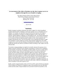
Analysis of water quality data collected from the Doris NorthProject in NunavutCarl James Schwarz (P.Stat. (Can, U.S.))Department of Statistics and Actuarial ScienceSimon Fraser UniversityBurnaby, BC V5A 1S6cschwarz@stat.sfu.ca2011-04-071. IntroductionThis report discusses the analysis of water quality data collected for the Doris NorthProject in Nunavut. The data for this analysis was provided by Rescan EnvironmentalServices Ltd.There are three aspects to the water quality monitoring: streams, lakes, and marineenvironments. Monitoring was conducted sporadically in the 1990s, more intensely inthe 2000’s, and construction started in 2010.Water quality samples were collected at various times in the year and at variouslocations. Within a year, sampling was often (not always) available monthly from Juneto September. In some cases, duplicate samples from the same date and location onthe body of water were taken. Many water quality parameters were measured, and asubset of 18 parameters (e.g. metals, pH, alkalinity, etc) were selected for analysis.Some of the measured values were below the detection limit (which changes overtime) and only the fact that the measurement is below the detection limit is recordedin these cases.The objective of this report is to examine if there is evidence of a change in the meanlevels of the water quality parameters in 2010 (when construction started) comparedto the pre-construction period in bodies of water close to Project constructionactivities (the Project or exposure waterbodies) relative to bodies of water notimpacted by the construction (the reference waterbodies).1.1 Streams:Five streams were monitored, two of which are treated as reference streams(Reference B Outflow and Reference D Outflow) and three as Project streams (DorisOutflow, Roberts Outflow, and Little Roberts Outflow). Monitoring of the Projectstreams started with a few measurements in 1996, 1997 and 2000, but moresystematic monitoring in all years since 2003. The Reference B Outflow stream hasmeasurements in 2009 and 2010, but the Reference D Outflow stream only has1

measurements in 2010. The within-year timing of the samples was divided into early(June or earlier) or late (July or later) sampling seasons.1.2 MarineThree locations were monitored, one of which is treated as the reference site. Oneof the Project sites (RBE) has been monitored since 2004; the second Project site(RBW) has been monitored since 2009; the reference site (REF-AEMP) has also beenmonitored since 2009.Historical samples were usually collected in surface layer or mid-column.Occasionally, historical marine samples were collected from the lower layer of thewater column or just above the sediment, but these samples were excluded from theanalysis because 2010 samples were only collected from the surface layer.The within-year timing of the sample was divided into early (June or earlier) or late(July or later) sampling seasons. The reference site was only sampled in the lateseason in all years.Many of the detection limits in 2010 were higher than in past years with most readingsfor several parameters now below detection limits. This will make it difficult todetect any Project impacts in 2010.1.3 LakesLakes were divided into large and small lakes and a separate analysis is done for eachsize category.1.3.1 Small LakesOnly two lakes were monitored in the small lake category with the Project lake (LittleRoberts Lake) being monitored since 1995, but the reference lake (Reference Lake D)only monitored in 2010. Unfortunately, this will severely limit the analyses that canbe done for this size category. All historical and 2010 samples collected in the smalllakes were collected from either the surface or middle of the water column.The within-year timing of the sample was divided into early (June or earlier) or late(July or later) sampling seasons.1.3.2 Large LakesThe large lake category included two Project lakes and one reference lake. OneProject lake (Doris Lake North) was monitored in 1995 and then from 2003 onwards;the second Project lake (Doris Lake South) was only monitored in 1995 and then in2009 and 2010; the reference lake (Reference Lake B) was monitored only in 2009 and2010.2

Historical data were collected from two depth strata: Surface and Deep. Somesamples from 1995 had an unknown depth zone and these were classified also ascoming from the surface. Both zones were sampled in 2009 and 2010 in all lakes, butonly surface water was sampled in 1995 and 2003 in the Project lakes. Because therewas little evidence of vertical chemical stratification, samples from all depths wereincluded in the analysis, and no depth effect was introduced in the analysis.The within-year timing of the sample was divided into early (June or earlier) or late(July or later) sampling seasons.2. Analysis Methods2.1 AssumptionsThere are several assumptions made for the analyses in this section. The keyassumption is that the samples taken are a random sample of the body’s water qualityfor that monitoring period (e.g., for that month in that year when measured) and ofthe sampling location. There is no way to assess this assumption other than by acareful consideration of the landscape and sampling protocol.Another necessary assumption is that missing data (e.g., a stream was not measuredin a month in a particular year) is missing completely at random (MCAR) so that thereis no information about the water quality from the “missingness”. This assumptioncould be violated if, for example, samples were not taken because it was known thatwater quality was compromised on the selected sampling date. There is no way toassess this assumption except by carefully considering why data was not collected ona particular date. If, for example, data were not collected because the sampling vialbroke in transit, this is likely a case of MCAR.It is further assumed that the water columns of all sampled waterbodies arecompletely mixed so that depth effects can be ignored. This assumption was verifiedby examining the raw sample means at various depths, and fitting statistical modelsto examine the effects of depth, and few depth effects were seen.2.2 Replicate samplesReplicate samples collected within the same day and at the same depth are treatedas pseudo-replicates (Hurlbert, 1984) and values are averaged before furtheranalyses. This will be an approximate analysis (compared to actually modellingreplicated values as nested within a particular day), but given the high variabilityseen for most of the readings, the reported results should be insensitive to thisaveraging.3

2.3 Dealing with censoring (values below detection limits)The proportion of data with readings below the detection limit varies by waterbodyand by chemical parameter. The analyses below follow the advice of McBride (2005,Section 11.4.3).• When the dataset has a small number of below detection values, we replacethese values by the detection limit or by ½ of the detection limit andconducted the analyses under both substitutions and note if the results differmaterially in either case. In this report, only the results from substituting ½ ofdetection limit for censored values are presented as analyses using thedetection limit as the substituted value did not differ in any great way.• When the dataset has mostly values below the detection limit (e.g., more thanabout 70% below detection limit), there is very little that can be done as thereis essentially no information (other than the values are below the detectionlimit). The analyses will be performed as above, but interpreting the resultsshould be done carefully. Helsel (2005) has other suggestions for analysis (e.g.,comparing the proportions below the detection limits) but these tests willrequire much larger sample sizes than available here.• When there are intermediate amount of censoring, a more complex analysiscan be conducted that fully integrates the information from the censoredvalues with the known values. This is most easily done using Bayesian methodsusing MCMC methods as likelihood methods would require integration of thelikelihood for each censored value over and above dealing with the otherrandom effects in the model. There is currently, no readily available softwareavailable for the latter. Fortunately, most chemical parameters fall into one ofthe two previous categories.It should be noted that for data collected in the late 1990’s, the detection limits wereconsiderably larger than the detection limits available for more modern sampling(often 5x or 6x larger). Consequently, there is little to be gained from using this veryearly data and it will often be removed prior to analysis and treated as outliers asnoted in the sections below.2.4 TransformationsFor all water quality parameters, the values were fairly homogeneous and no obvioustransformation was suggested, i.e., metals analyzed on the ppm scale and pHmeasured on the log-scale.2.5 Dealing with sparse data in some classifications such as seasonIn models with season effects, samples were not always collected during all seasons ofall years or periods. In these cases, interaction effects involving season cannot be fitbut additive models can still be fit.4

presented in this report because of the very small number of statistically significantdifferences found, but are available if needed.The key disadvantage of this model is that changes over time may be unrelated to theeffects of the Project, e.g., the water quality readings in 2010 could be worse thanexpected because of long term climate change that is unrelated to the Project.Consequently, if a statistically significant effect is detected, it will require furtherinvestigation.2.6.2 BACI analysisThe standard method to assess an environmental impact is through a Before-After-Control-Impact (BACI) analysis (Smith, 2002). The analysis of these designs looks fornon-parallelism in response over time between the Project and reference streams. ABACI analysis was performed for each Project waterbody versus the correspondingreference waterbody.The formal statistical model (in standard shorthand notation) is:WQ = Period Season Period*Season Class Period*Class Year(Period)-Rwhere WQ is the mean water quality reading on a date; Period is the effect of period(before or after construction); Season is the effect of season (early or late);Period*Season is the interaction between the period and season effects (i.e., is thechange in the mean over the two periods the same for both seasons); Class is theeffect of water body classification (Project or reference); Period*Class is the BACIeffect of interest (i.e., is the effect of Period the same (parallel) for both classes ofwater body); and Year(Period) is the random year effect for multiple years withineach period. If there were multiple reference bodies, a term Body(Class)-R will alsobe added to the model and so the change in the mean for the Project stream iscompared to the average change in the mean for the reference bodies.The key parameter of interest is the Period*Class effect as this measures the amountof non-parallelism between the changes in the mean (After-Before) over the twoclasses of water bodies (Project or reference).In some cases, not all bodies are measured in every year. This information doesprovide information about the year-to-year variation when compared with otheryears.The BACI estimate is computed as the “difference in the differences”, i.e.,BACI = ( µ PA− µ PB ) − ( µ RA− µ RB )where µ PBis the mean water quality reading in the Project class after Projectconstruction with a similar definition for the other population means. The BACIcontrast is estimated by replacing the population means above by the model-basedestimates. Estimated differences close to 0 would indicate no evidence of nonparallelism.6

Note that the hypothesis that the BACI contrast has the value of zero is identical tothe hypothesis that the Period*Class interaction is zero with identical p-values.Consequently, only the results for the BACI contrast are reported in the tables.This model was fit using a mixed-model ANOVA using Proc Mixed in SAS 9.2.Note that as in any BACI analysis without replicated sites in the two classes, theresults are specific to those sites used and cannot be extrapolated to other sites. Theresults may be specific to these particular sites for some site-specific factor such asgeomorphology.2.6.3 Multivariate approachesAll of the approaches above analyze each chemical parameter independently of eachother. However, the chemical constituents do not occur independently of each other,and presumably higher power would result if a multivariate approach were used.However, because of the censoring and missing data, no simple multivariate approachis possible and such an analysis would likely require the use of a full Bayesian MCMCapproach. This has not been attempted in this report.3. Results3.1 Stream DataA summary of the amount of censoring (below detection limit) for the stream data isfound in Table Stream-1. High levels of censoring in all streams were found for theCd, Hg, Nitrate, and Ra parameters and the results of the analyses for theseparameters will be non-informative and should be discarded.High level of censoring for TSS, Ammonia, Mo, Pb, and Zn was found in one or all ofthe reference streams but a lower proportion of censored values were found inProject streams. In these cases, the results will require further investigation to ensurethat the censoring is not causing an artifact in the results.Preliminary plots of the data showed some outliers, primarily from readings in thelate 1990’s where the detection limit was much higher than in recent times (TableStream-2). These were discarded as such a large detection limit compared to morerecent data provides little information on the actual value. Some other outliers thatwere not related to high detection limits were also discarded.The results from the analysis that compared the means before and after Projectconstruction are presented in Table Stream-3. There was evidence of a change in themean between the before and after periods for CN (intermediate amounts of7

censoring) in all streams where data were present, Al in Doris OF stream, and Fe inRoberts OF stream.The results of the BACI comparison of each Project stream against the referencestreams (Table Stream-4) failed to find evidence of a differential response in themean between Project and reference streams over the before and after periods.Unfortunately, CN was not measured in reference streams prior to Project impact,and so a BACI comparison cannot be performed for this parameter.3.2 Marine DataA summary of the amount of censoring (below detection limit) for the site data isfound in Table Marine-1. High levels of censoring in all sites were found for the Hg,Nitrate, and Ra parameters and the results of the analyses for these parameters willbe non-informative and should be discarded. As noted earlier, many of the 2010readings were also censored at a higher detection limit than in previous years.Preliminary plots of the data showed some outliers as shown in Table Marine-2 whichwere removed prior to analysis. Of particular concerns are As readings at the RBE sitewhich were substantially elevated prior to 2007 but then fall to near or belowdetection limits post 2007. This may indicate a change in sampling methodology orphysical processes within this marine site.The results from the analysis that compared the means before and after Projectconstruction are presented in Table Marine-3. There was evidence of a change in themean between the before and after periods for Pb in RBE (intermediate amount ofcensoring).The results of the BACI comparison (Table Marine-4) failed to find evidence of adifferential response in the mean between any marine Project site and the referencesite over the before and after periods. As the increased detection limit occurred in allstreams in 2010, this common “effect” may have masked any changes.3.3 Small lakesA summary of the amount of censoring (below detection limit) for the small lake datais found in Table Slake-1. High levels of censoring in all streams were found for Cd,Hg, Nitrate, and Ra parameters and the results of the analyses for these parameterswill be non-informative and should be discarded.Preliminary plots of the data showed some outliers that were primarily censored datafrom the early 1990s. The observations listed in Table Slake-2 were discarded prior toanalysis to ensure that these observations don’t artificially inflate the varianceestimates leading to a reduced power to detect effects.8

There was evidence of a change in the mean of the CN parameter between thebefore and after period in the Project lakes (Table Slake-3). In this case, all of thereadings prior to Project construction were at or below detection limit and none ofthe readings post-construction are below the detection limit.Because only the Project lake was measured before and after construction started, noBACI analysis is possible.3.5 Large lakesA summary of the amount of censoring (below detection limit) for the large lake datais found in Table Llake-1. High levels of censoring in all streams were found for Cd,Nitrate, and Ra parameters and the results of the analyses for these parameters willbe non-informative and should be discarded. High levels of censoring were also foundfor the reference lake only in Mo, TSS, and Zn. This will make the BACI comparisondifficult to interpret.Preliminary plots of the data showed some potential outliers (Table Llake-2) thatwere excluded from the analysis.There was evidence of a difference in the means between the before and afterperiods for As in Doris North (the mean As appears to have decreased in 2010), and CNin Doris North and Doris South (Table Llake-3).The BACI comparison (Table Llake-4) failed to find evidence of a differential responsein the mean between any Project site and the reference site over the before andafter periods. Unfortunately, CN was not measured in reference lakes prior to Projectimpact, and so a BACI comparison cannot be performed for this parameter.4. ReferencesHelsel, D.R. (2005). Nondetects and data analysis. Wiley:New York.Hurlbert S.H. (1984) Pseudoreplication and the design of ecological field experiments.Ecological Monographs, 54, 187-211.McBride, G.B. (2005). Using statistical methods for water quality management. Wiley:New York.Smith, E. P. (2002). BACI Design. Encyclopedia of Environmetrics, Wiley: New York.9

Table Stream-1. Summary of the proportion censored (beforeoutliers removed) in each stream for each chemicalparameter.ParameterDoris OFPropcensoredLittleRobertsOFPropcensoredStreamRef. BOFPropcensoredRef. DOFPropcensoredRobertsOFPropcensored10Al 0.00 0.00 0.00 0.00 0.00Alk 0.00 0.00 0.00 0.00 0.00Ammonia 0.32 0.31 0.64 0.50 0.24As 0.05 0.03 0.00 0.00 0.00CN 0.75 0.52 0.00 0.13 0.62Cd 0.79 0.69 1.00 1.00 0.69Cu 0.00 0.00 0.00 0.00 0.00Fe 0.00 0.00 0.00 0.00 0.00Hardness 0.00 0.00 0.00 0.00 0.00Hg 0.86 0.89 1.00 1.00 0.76Mo 0.05 0.00 0.86 0.00 0.00Ni 0.05 0.00 0.14 0.13 0.00Nitrate 0.86 0.95 0.50 0.75 0.83Pb 0.19 0.21 1.00 0.25 0.07Ra 0.82 0.88 0.88 0.75 0.93TSS 0.14 0.08 0.93 0.88 0.07

Table Stream-1. Summary of the proportion censored (beforeoutliers removed) in each stream for each chemicalparameter.11ParameterDoris OFPropcensoredLittleRobertsOFPropcensoredStreamRef. BOFPropcensoredRef. DOFPropcensoredRobertsOFPropcensoredZn 0.29 0.33 1.00 1.00 0.21pH 0.00 0.00 0.00 0.00 0.00

Table Stream-2. Summary of potential outliers from the stream data. Censored values were replaced by ½ of the detection limit.Stream Parameter Year Date Rep Reading Censored*Doris OF Ammonia 1997 19JUL97 1 1.359800 0Doris OF Ammonia 1997 19JUL97 2 1.402400 0Doris OF Ammonia 1997 20AUG97 1 1.353300 0Doris OF As 1996 22AUG96 1 0.003000 0Doris OF Cd 1996 22AUG96 1 0.000025 1Doris OF Cd 1997 19JUN97 1 0.000100 1Doris OF Cd 1997 19JUL97 1 0.000100 1Doris OF Cd 1997 19JUL97 2 0.000100 1Doris OF Cd 1997 20AUG97 1 0.000100 1Doris OF Cd 2000 20JUN00 1 0.000025 1Doris OF Cd 2000 20JUN00 2 0.000025 1Doris OF Cd 2000 14SEP00 1 0.000025 1Doris OF Cd 2000 14SEP00 2 0.000025 1Doris OF Cd 2004 24JUN04 1 0.000025 1Doris OF Hg 1997 20AUG97 1 0.000025 1Doris OF Hg 2000 20JUN00 1 0.000025 1Doris OF Hg 2000 20JUN00 2 0.000025 1Doris OF Hg 2000 14SEP00 1 0.000025 1Doris OF Hg 2000 14SEP00 2 0.000025 1Doris OF Hg 2003 28JUL03 1 0.000025 1Doris OF Mo 1997 19JUN97 1 0.000500 1Doris OF Mo 1997 19JUL97 1 0.000500 1Doris OF Mo 1997 19JUL97 2 0.000500 112

Table Stream-2. Summary of potential outliers from the stream data. Censored values were replaced by ½ of the detection limit.13Stream Parameter Year Date Rep Reading Censored*Doris OF Mo 1997 20AUG97 1 0.000500 1Little Roberts OF Hg 2003 28JUL03 1 0.000025 1Ref. B OF Hg 2010 19JUN10 1 0.000025 1Ref. B OF Hg 2010 19JUN10 2 0.000025 1Ref. D OF Hg 2010 18JUN10 1 0.000025 1Ref. D OF Hg 2010 18JUN10 2 0.000025 1Roberts OF Hg 2010 18JUN10 1 0.000025 1Roberts OF Hg 2010 18JUN10 2 0.000025 1* 1 = yes (censored, i.e. below the detection limit); 0 = not censored.

Table Steam-3. Summary of test for no difference in mean between before and after periods for chemical parameters measured on streams.To reduce the number of false positives, a smaller alpha level ( .01) was used to screen for effects and p-values < .01 are bolded.Seasonal effects are not of interest. In some cases, no analysis can be done because of the high degree of censoring, no variation in results withinseasons or years, or high levels of censoring.ParameterEffectperiod period*season seasonAvg Propstream stream streamcensoredLittleLittleLittleafterDoris Roberts Ref. B Ref. D Roberts Doris Roberts Ref. B Ref. D Roberts Doris Roberts Ref. B Ref. D RobertsremovalOF OF OF OF OF OF OF OF OF OF OF OF OF OF OFofoutliers Pr > F Pr > F Pr > F Pr > F Pr > F Pr > F Pr > F Pr > F Pr > F Pr > F Pr > F Pr > F Pr > F Pr > F Pr > FAl 0.00 0.006 0.458 0.316 . 0.254 0.368 0.850 0.545 . 0.309 0.204

Table Steam-3. Summary of test for no difference in mean between before and after periods for chemical parameters measured on streams.To reduce the number of false positives, a smaller alpha level ( .01) was used to screen for effects and p-values < .01 are bolded.Seasonal effects are not of interest. In some cases, no analysis can be done because of the high degree of censoring, no variation in results withinseasons or years, or high levels of censoring.Effectperiod period*season seasonAvg Propstream stream streamcensoredLittleLittleLittleafterDoris Roberts Ref. B Ref. D Roberts Doris Roberts Ref. B Ref. D Roberts Doris Roberts Ref. B Ref. D RobertsremovalOF OF OF OF OF OF OF OF OF OF OF OF OF OF OFofoutliers Pr > F Pr > F Pr > F Pr > F Pr > F Pr > F Pr > F Pr > F Pr > F Pr > F Pr > F Pr > F Pr > F Pr > F Pr > FRa 0.85 0.950 0.961 . . 0.209 0.742 0.961 . . 0.209 0.280 0.530 0.667 0.184 0.209TSS 0.42 0.169 0.567 0.703 . 0.087 0.341 0.384 0.703 . 0.649 0.206 0.065 0.703 0.667 0.112Zn 0.28 0.589 0.339 . . 0.562 0.813 0.094 . . 0.694 0.813 0.094 . . 0.155pH 0.00 0.317 0.207 0.587 . 0.308 0.840 0.123 0.584 . 0.427 0.451 0.042 0.917 0.573 0.11515

Table Stream-4. Summary of BACI comparisons for individual Project sites in the stream study. Some comparisons were not possiblebecause data were missing or data were all constant over time.ParameterProject StreamDoris Little Robert RobertBACI est BACI SE p-value BACI est BACI SE p-value BACI est BACI SE p-valueAl 0.1347 0.1195 0.264 -0.0101 0.0943 0.916 0.0140 0.1542 0.928Alk -1.0661 2.1971 0.629 -0.8278 1.9361 0.672 -0.2872 2.0530 0.891Ammonia 0.0039 0.0082 0.639 -0.0002 0.0073 0.975 -0.0013 0.0065 0.848As -0.0001 0.0001 0.542 -0.0001 0.0001 0.295 -0.0002 0.0001 0.075CN . . . . . . . . .Cd 0.0000 0.0000 0.334 0.0000 0.0000 0.928 0.0000 0.0000 0.873Cu 0.0003 0.0004 0.403 0.0002 0.0003 0.506 -0.0001 0.0003 0.752Fe 0.1618 0.1527 0.294 0.0155 0.1073 0.886 0.1232 0.1289 0.346Hardness 2.2984 4.6012 0.619 1.3562 4.3081 0.755 1.2482 3.1708 0.697Hg . . . 0.0000 0.0000 0.634 . . .Mo 0.0000 0.0000 0.892 -0.0000 0.0000 0.988 -0.0000 0.0000 0.559Ni 0.0002 0.0002 0.426 -0.0000 0.0001 0.836 0.0000 0.0001 0.757Nitrate 0.0024 0.0031 0.434 0.0028 0.0018 0.133 -0.0018 0.0087 0.842Pb 0.0000 0.0001 0.523 -0.0000 0.0001 0.546 -0.0000 0.0001 0.856Ra . . . . . . . . .TSS 3.9496 3.1976 0.221 -3.6050 2.0385 0.085 1.9481 1.6903 0.265Zn -0.0012 0.0021 0.549 -0.0010 0.0013 0.445 -0.0018 0.0018 0.340pH 0.1386 0.2650 0.603 0.1319 0.1799 0.468 0.2217 0.3746 0.57216

Table Marine-1. Summary of proportion ofmeasurements below detection limit (beforeoutliers removed) for marine sampling.17SiteParameterRBE RBW REF-AEMPPropcensoredPropcensoredPropcensoredAl 0.07 0.33 0.00Alk 0.00 0.00 0.00Ammonia 0.50 1.00 0.40As 0.24 0.56 0.60CN 0.55 0.17 0.00Cd 0.48 0.56 0.60Cu 0.17 0.33 0.40Fe 0.17 0.44 0.20Hardness 0.00 0.00 0.00Hg 0.78 1.00 1.00Mo 0.11 0.11 0.00Ni 0.21 0.11 0.40Nitrate 0.78 0.67 1.00Pb 0.48 0.78 1.00Ra 0.86 1.00 1.00TSS 0.04 0.11 0.00Zn 0.28 0.67 0.80pH 0.00 0.00 0.00

Table Marine-2. Summary of potential outliers from the marine data. Censored values have been replaced by ½ of detection limit.Site Parameter Year Date Rep Reading Censored*RBE Al 2005 21JUL05 1 0.989000 0RBE Ammonia 2007 23JUL07 1 0.214000 0RBE As 2004 19JUL04 1 0.008020 0RBE As 2004 14AUG04 1 0.015200 0RBE As 2004 16AUG04 1 0.013100 0RBE As 2004 09SEP04 1 0.022300 0RBE As 2005 21JUL05 1 0.004730 0RBE As 2005 18AUG05 1 0.022100 0RBE As 2005 14SEP05 1 0.021200 0RBE As 2006 31MAY06 1 0.015200 0RBE As 2006 20JUL06 1 0.013300 0RBE As 2006 12AUG06 1 0.025600 0RBE As 2006 11SEP06 1 0.023680 0RBE CN 2007 23JUL07 1 2.500000 1RBE Ni 2006 11SEP06 1 0.006500 0RBE Ra 2004 14AUG04 1 0.020000 0REF-AEMP Nitrate 2010 13JUL10 1 1.250000 1*1 = yes (censored, i.e. below the detection limit); 0 = not censored.18

19Table Marine-3. Summary of test for no difference in mean between before and after periods for chemicalparameters measured on marine areas. To reduce the number of false positives, a smaller alpha level ( .01)was used to screen for effects with statistically significant differences bolded. Seasonal effects are not ofinterest.ParameterEffectAvg Propcensoredperiod period*season seasonafterSite Site SiteremovalofRBE RBW REF-AEMP RBE RBW REF-AEMP RBE RBW REF-AEMPoutliers Pr > F Pr > F Pr > F Pr > F Pr > F Pr > F Pr > F Pr > F Pr > FAl 0.14 0.649 0.750 0.362 0.308 0.761 . 0.214 0.747 .Alk 0.00 0.090 . . 0.993 . . 0.034 0.277 .Ammonia 0.46 0.305 . 0.492 0.653 . . 0.653 . .As 0.51 0.728 0.059 0.037 0.612 0.089 . 0.456 0.130 .CN 0.23 0.193 . . 0.116 . . 0.116 0.030 .Cd 0.55 0.320 0.166 0.105 0.891 0.307 . 0.878 0.185 .Cu 0.30 0.617 0.643 0.657 0.867 0.654 . 0.337 0.754 .Fe 0.27 0.968 0.696 0.478 0.712 0.775 . 0.207 0.750 .Hardness 0.00 0.392 0.929 . 0.847 . . 0.172 0.176 .Hg 0.78 0.258 . . 0.487 . . 0.487 . .Mo 0.07 0.369 0.137 0.516 0.794 0.040 . 0.110 0.017 .Ni 0.24 0.812 0.829 0.596 0.787 0.224 . 0.370 0.434 .Nitrate 0.81 0.702 0.827 0.667 0.726 0.738 . 0.404 0.981 .Pb 0.75 0.003 0.294 0.423 0.394 0.899 . 0.831 0.673 .Ra 0.92 0.220 . . . . . 0.420 . .

Table Marine-3. Summary of test for no difference in mean between before and after periods for chemicalparameters measured on marine areas. To reduce the number of false positives, a smaller alpha level ( .01)was used to screen for effects with statistically significant differences bolded. Seasonal effects are not ofinterest.20ParameterEffectAvg Propcensoredperiod period*season seasonafterSite Site SiteremovalofRBE RBW REF-AEMP RBE RBW REF-AEMP RBE RBW REF-AEMPoutliers Pr > F Pr > F Pr > F Pr > F Pr > F Pr > F Pr > F Pr > F Pr > FTSS 0.05 0.956 0.853 0.088 0.114 0.439 . 0.453 0.628 .Zn 0.58 0.901 0.127 0.457 0.946 0.671 . 0.450 0.815 .pH 0.00 0.707 0.018 0.092 0.851 0.087 . 0.826 0.008 .

Table Marine-4. Summary of BACI comparisons for individual Project sites in the marine areas.Some comparisons were not possible because data were missing or data were all constant over time.21Marine Project SiteRBERBWBACI est BACI SE p-value BACI est BACI SE p-valueParameterAl 0.1030 0.1439 0.482 0.0903 0.1910 0.661Alk . . . . . .Ammonia 0.0029 0.0090 0.749 0.0030 0.0036 0.452As -0.0004 0.0002 0.037 -0.0002 0.0002 0.356CN . . . . . .Cd -0.0000 0.0000 0.611 -0.0000 0.0000 0.879Cu -0.0004 0.0017 0.841 0.0001 0.0007 0.933Fe 0.0155 0.2548 0.952 0.0636 0.2220 0.789Hardness . . . . . .Hg . . . . . .Mo -0.0001 0.0028 0.969 0.0040 0.0017 0.075Ni -0.0003 0.0009 0.711 -0.0000 0.0006 0.994Nitrate -0.0752 0.1303 0.571 . . .Pb -0.0000 0.0002 0.969 0.0000 0.0004 1.000Ra . . . . . .TSS -1.1290 9.9793 0.911 0.7167 8.7575 0.939Zn 0.0005 0.0027 0.865 0.0017 0.0019 0.411pH -0.0514 0.3195 0.874 -0.0500 0.0478 0.355

Table Slake-1. Summary of theproportion censored (beforeoutliers are removed) in eachsmall lake for each chemicalparameter.22LakeParameterLittleRobertsPropcensoredReferenceDPropcensoredAl 0.00 0.00Alk 0.03 0.00Ammonia 0.27 0.83As 0.09 0.00CN 0.61 0.00Cd 0.73 1.00Cu 0.00 0.00Fe 0.00 0.00Hardness 0.00 0.00Hg 0.70 1.00Mo 0.06 0.00Ni 0.03 0.00Nitrate 0.70 0.67Pb 0.09 0.00Ra 0.80 0.83TSS 0.21 1.00

Table Slake-1. Summary of theproportion censored (beforeoutliers are removed) in eachsmall lake for each chemicalparameter.23LakeParameterLittleRobertsPropcensoredReferenceDPropcensoredZn 0.21 0.83pH 0.00 0.00

Table Slake-2. Summary of potential outliers from the small lake data. Censored values have been replaced by ½ of the detection limit.Lake Parameter Year Date Rep Reading Censored*Little Roberts Ammonia 2007 24MAY07 1 0.240000 0Little Roberts Cd 1995 07JUN95 1 0.000100 1Little Roberts Cd 1996 27AUG96 1 0.000025 1Little Roberts Cd 1996 27AUG96 2 0.000025 1Little Roberts Cd 1997 15JUL97 1 0.000100 1Little Roberts Cd 1997 15JUL97 2 0.000100 1Little Roberts Fe 2007 24MAY07 1 1.700000 0Little Roberts Hg 2003 27JUL03 1 0.000230 0Little Roberts Mo 1997 15JUL97 1 0.000500 1Little Roberts Mo 1997 15JUL97 2 0.000500 1Little Roberts Nitrate 2004 13SEP04 1 5.300000 0Little Roberts Ra 2004 13SEP04 1 0.060000 0* 1 = yes (censored, i.e. below the detection limit); 0 = not censored.24

25Table Slake-3. Summary of test for no difference in mean between before and afterperiods for chemical parameters measured on small lakes. To reduce the number offalse positives, a smaller alpha level ( .01) was used to screen for effects andstatistically significant effects are bolded. Seasonal effects are not of interest.ParameterEffectAvg Propperiod period*season seasoncensored Lake Lake LakeafterLittle Reference Little Reference Little ReferenceremovalRoberts D Roberts D Roberts Dofoutliers Pr > F Pr > F Pr > F Pr > F Pr > F Pr > FAl 0.00 0.593 . 0.565 . 0.477 0.657Alk 0.01 0.882 . 0.903 . 0.003 0.029Ammonia 0.56 0.243 . 0.113 .

Table Slake-3. Summary of test for no difference in mean between before and afterperiods for chemical parameters measured on small lakes. To reduce the number offalse positives, a smaller alpha level ( .01) was used to screen for effects andstatistically significant effects are bolded. Seasonal effects are not of interest.26EffectAvg Propperiod period*season seasoncensored Lake Lake LakeafterLittle Reference Little Reference Little ReferenceremovalRoberts D Roberts D Roberts Dofoutliers Pr > F Pr > F Pr > F Pr > F Pr > F Pr > FRa 0.86 . . . . . .TSS 0.36 0.165 . 0.072 . 0.398 .Zn 0.34 0.457 . 0.633 . 0.235 .pH 0.00 0.012 . 0.234 . 0.287 0.636

Table Llake-1. Summary of the proportioncensored (before outliers removed) ineach large lake for each chemicalparameter.27ParameterDorisNorthPropcensoredLakeDorisSouthPropcensoredReferenceBPropcensoredAl 0.00 0.13 0.00Alk 0.00 0.00 0.00Ammonia 0.28 0.73 0.23As 0.08 0.33 0.15CN 0.66 0.33 0.00Cd 0.74 0.93 0.77Cu 0.01 0.00 0.08Fe 0.05 0.00 0.69Hardness 0.00 0.00 0.00Hg 0.59 1.00 0.92Mo 0.07 0.20 0.85Ni 0.00 0.00 0.38Nitrate 0.68 0.60 0.69Pb 0.17 0.20 0.31Ra 0.89 1.00 0.75TSS 0.12 0.33 1.00

Table Llake-1. Summary of the proportioncensored (before outliers removed) ineach large lake for each chemicalparameter.28ParameterDorisNorthPropcensoredLakeDorisSouthPropcensoredReferenceBPropcensoredZn 0.21 0.47 0.85pH 0.00 0.00 0.00

Table Llake-2. Summary of potential outliers from the large lake data. Censored values have been replaced by ½ of detection limit.Lake Parameter Year Date Rep Reading Censored*Doris North As 1995 20AUG95 - 0.003000 0Doris North Fe 1995 20AUG95 - 0.720000 0Doris North Ni 2005 19JUL05 1 0.028300 0Doris North Pb 2004 05JUN04 1 0.006690 0Doris North Ra 2004 10SEP04 1 0.060000 0Doris North TSS 2004 10SEP04 1 29.000000 0Doris South Al 2009 24APR09 1 0.329000 0Doris South Fe 2009 24APR09 1 0.629000 0* 1 = yes (censored, i.e. below the detection limit); 0 = not censored.29

Table Llake-3. Summary of test for no difference in mean between before and after periods forchemical parameters measured on large lakes. To reduce the number of false positives, a smalleralpha level ( .01) was used to screen for effects and statistically significant effects are bolded.Seasonal effects are not of interest.ParameterEffectAvg Propperiod period*season seasoncensoredlake lake lakeafterDoris Doris Reference Doris Doris Reference Doris Doris ReferenceremovalNorth South B North South B North South Bofoutliers Pr > F Pr > F Pr > F Pr > F Pr > F Pr > F Pr > F Pr > F Pr > F30Al 0.05 0.643 0.240 0.230 0.490 0.173 0.194 0.001 0.004 0.098Alk 0.00 0.520 0.497 0.578 0.523 0.273 0.845 0.042 0.004 0.161Ammonia 0.41 0.127 0.088 0.336 0.395 0.130 0.584 0.620 0.151 0.337As 0.19 0.006 0.625 0.101 0.062 0.135 0.130 0.135 0.108 0.826CN 0.33 0.009 0.001 . 0.890 . . 0.577 0.124 0.318Cd 0.84 0.519 0.802 . 0.590 0.732 . 0.590 0.534 .Cu 0.03 0.922 0.458 0.186 0.875 0.811 0.581 0.095

Table Llake-3. Summary of test for no difference in mean between before and after periods forchemical parameters measured on large lakes. To reduce the number of false positives, a smalleralpha level ( .01) was used to screen for effects and statistically significant effects are bolded.Seasonal effects are not of interest.31ParameterEffectAvg Propperiod period*season seasoncensoredlake lake lakeafterDoris Doris Reference Doris Doris Reference Doris Doris ReferenceremovalNorth South B North South B North South Bofoutliers Pr > F Pr > F Pr > F Pr > F Pr > F Pr > F Pr > F Pr > F Pr > FTSS 0.23 0.644 0.533 . 0.542 0.419 . 0.008 0.014 .Zn 0.34 0.548 0.354 . 0.466 0.376 . 0.466 0.381 .pH 0.00 0.242 0.579 0.389 0.877 0.460 0.959 0.734 0.296 0.550

Table Llake-4. Summary of BACI comparisons for individual Project sites in the large lake areas. Some comparisons were not possiblebecause data were missing or data were all constant over time.Large Project Lake32Doris NorthDoris SouthBACI est BACI SE p-value BACI est BACI SE p-valueParameterAl 0.0026 0.0186 0.890 0.0481 0.0162 0.021Alk 0.3364 3.6799 0.928 -0.0349 2.0004 0.987Ammonia -0.0132 0.0062 0.043 -0.0239 0.0118 0.077As -0.0003 0.0001 0.017 -0.0001 0.0000 0.193CN . . . . . .Cd 0.0000 0.0000 0.950 0.0000 0.0001 0.535Cu -0.0003 0.0006 0.679 -0.0001 0.0003 0.687Fe 0.0275 0.0467 0.561 0.0665 0.0277 0.047Hardness 2.6225 3.1301 0.411 3.7481 2.1379 0.123Hg 0.0000 0.0000 0.039 0.0000 0.0000 0.089Mo 0.0000 0.0000 0.273 0.0000 0.0000 0.789Ni -0.0001 0.0001 0.494 -0.0002 0.0002 0.386Nitrate -0.0047 0.0201 0.816 -0.0237 0.0092 0.033Pb -0.0005 0.0003 0.145 -0.0007 0.0005 0.208Ra . . . . . .TSS 0.2650 1.5617 0.866 2.0250 1.4145 0.190Zn -0.0044 0.0193 0.823 -0.0512 0.0550 0.378pH -0.0347 0.4991 0.945 -0.2826 0.2902 0.362