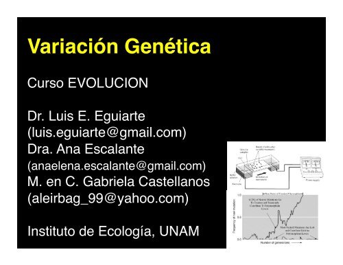
Variación Genética - Instituto de Ecología

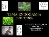
Gen: unidad de herencia que setrasmite de padres a hijosLocus/ loci: lugar en el cromosomadonde se localiza el gen; lo usamoscomo sinónimo de gen.A veces llamamos genes a seccionesno-codificadoras (práctico, útiles...).ALELOS: las diferentes formas de ungen dado (A, a, a1, a2, a´, a*, etc.).

Diploide: organismos con 2 copias de cada gene.Haploides: 1 sola copia (bacterias)Poliploides: varias copias (más de 2);tetraploides: 4, etc. Pueden ser autopoliploides(las 4 copias de un ancestro), o alopoliplodes (2de uno y 2 de otro).Genoma: una de las copias de todos los genes...(se usa a veces para mitocondria, cloroplasto,etc.).Genotipo: constitución genética de losorganismos: Homócigos, las dos copias delgen (loci) iguales AA, aa.Heterócigo: las dos copias distintas.

Gregor MendelX !X !Púrpura!Blanco!Púrpura!Blanco!X !‏!(‏Aa‏)‏ Púrpura‏!(‏Aa‏)‏ Púrpura‏!(‏aa‏)‏ Blanco ‏!(‏Aa‏)‏ Púrpura ‏!(‏Aa‏)‏ Púrpura ‏!(‏AA‏)‏ Púrpura

Genes en autosomas y en cromosomassexuales, X y Y.Organismos haplo-diploides: himenópteros:machos haploides, hembras diploides.Mitocondria y cloroplasto: herencia materna,origen bacteriano.Cromosomas: piezas largas de ADN quesegregan de manera independiente de otroscromosomas. Dentro de un cromosomatenemos genes ligados entre si (se producengametos con igual ligamiento que en lospadres y otros con diferente ligamiento,RECOMBINACION.

Grupo de alelos ligados: haplotipo (se usamucho para mitocondria, cloroplasto).Wildtype: la forma silvestre, en genéticaclásica, la forma más común, el fenotipo“normal” (no mutante).ADN: 4 nucelótidos, codifica en tripletes, 20aminoácidos, 64 combinaciones.Mutaciones silenciosas o sinónimas: si nocambia el a.a.Mutaciones de reemplazo o no-sinónimas: lasque cambian el a.a.

Genetic material at the molecular level:!More complicated than what F, H & W (and even Kimura!)thought...!

Genetic material at the molecular level:!

Genetic material at the molecular level:!Nuclear Genome of de Arabidopsis thaliana !(Arabidopsis genome initiative, Nature (2000) 408:796-815.)!5 chromosomes (2n=10), 125 megabases (Mb)!Inbreeder, t=0 (self-pollinates)!25,498 genes (proteins) in 11,000 families!C. elegans 19,099, Drosophila 13,601 genes!H. sapiens 26,000 to 38,000 genes!4,405 genes in E. coli!Why so many in a plant?: Perhaps correlated to thecomplex biochemistry of the plants, related dosecondary compounds, defense to pathogens andherbivores, etc. !

Mobile elements!(transposable elements)!10% of the total nuclear genome(specially intergenic DNA 20% )!2,109 class I (replicate using aRNA intermediary ): incentromers!2,203 class II ( move directlyusing DNA): pericentric!

17% of Arabidopsis genome is in “tandemarrays”, the repeated genes one afteranother...!Most genes duplicated (not necessarily intandem), but seldom triplicated, etc.!This, coupled with molecular clock analysessuggests a polyploid (tetraployd ancestor, ca.112 Million YA).!Centromers: In chromosome 2, duplicated75% of the mitochondrial genome.!

Duplications in the 5 chromosomes of A. thaliana!

Average length of each gene: 1.9 kb (humans27kb per gene!!!):!Exons: 5.18 exons in average per gene,!Average size of each exon: 250 bp.!Average size of each intron: 170 bp.!ca. 600 bp of introns per gene!4 introns per gene in average.!5 exones, de 250 bp cu!total length 1.9 kb!4 introns, 170 bp each!

Three genomes in A. thalianaDifferent levels of resolution for differentevolutionary problems.

Genomes and genetics are morecomplicated than what the orignalpopulation geneticist (evenKimura!) thought...!But we can adjust our models andanalyses to study this incrediblerich databases!!!!

But to understand theideas and concerns ofKimura, we need first toreview the principles ofPopulation Genetics, both“classic” and “molecular”.!

Material genético: archivo del procesoevolutivo...a partir de este archivo, con la teoríaevolutiva, buenos datos ymuestreo, y buen análisisestadístico, podremos reconstruir elproceso evolutivo y entender lasfuerzas evolutivas que hanmodelado la diversidad yadaptaciones de los organismos...

VARIACIÓN GENÉTICA:1) EL PRIMER PASO EN TODO ESTUDIO EVOLUTIVA2) SI NO HAY VARIACIÓN, NO PUEDEN ACTUAR LASFUERZAS EVOLUTIVAS3) SEGÚN EL TIPO DE VARIACIÓN, SE VA ADETERMINAR LA EVOLUCIÓN ADAPTATIVA Y/OALEATORIA DE LAS POBLACIONES4) A PARTIR DE COMO SE DISTRIBUYEN DENTRO YENTRE LAS POBLACIONES, PODEMOS INFERIRLAS FUERZAS EVOLUTIVA Y LA HISTORIAPASADA (ESTA SERÍA “LA GRAN ILUSIÓN”, PEROA CADA VEZ PARECE MAS SEGURO QUE SI SEPUEDE LOGRAR!!!)

Classic Population Genetics:!Deals with the behavior of“simple” (mendelian) genes ina population...!The basic model considersone locus with only twoforms, two alleles:!A & a"

POBLACION IDEAL!modelo, poblaciones reales complicadas...!(caricatura de la realidad)!Pobl. ideal: no operan las fuerzas evolutivas)!Individuos que se pueden cruzar entre si en un !lugar y a un tiempo!Apareamientos al azar!Población grande.!Generación Discretas (no se sobreponen)!Todo esto forma la poza génica (GENETIC POOL)!

.AaAAAAAAAAAAAAAAAAAAAAAAAAAAAAaaAAAAAAaaAAAAAAAaAaAaAaAaAaAaAaAaAaAaAaAaAaAaAaAaAaAaAaAaaaaaaaaa aaaaaaaaaaaaaaaaaaaaaaaaESPECIEpoblaciones

N individuals!Frequencies de A= p 0 !Time 0!Evolution!Change in the allelefrequencies in time(T. Dobzhansky, 1941)!N individuals!Frequencies de A= p 1!N individuals!Frequencies de A = p t!Time 1!Time t!Hardy-WeinbergEquilibrium:!In a ideal population(large, sexualreproduction, diploid,random mating amongindividuals), the !allelic frequencies doNOT change !

The Evolutionary Forces violate the equilibrium of Hardy-!Weinberg and in consequence change the allelic frequencies !(and then generate Evolution).!!Genetic drift, !!Natural selection, !!Migration, !!Mutation!Other evolutionary process do not change the allelic !frequencies, but are relevant:!!Mating systems/ inbreeding!!Recombination!

Números Frecuencias F. alélicasgenotípicos genotípicasNAA P=NAA/Nt A= p p= P+1/2HNAaH=NAa/Nta= q q= Q+1/2HNaaQ=Naa/Nt______________________________SumasNt 1 1 p+q=1

Iniciales !gametos Sig. Generación !P=AA ! ! ! ! ! !pxp= AA!! ! !A = p!H=Aa ! ! ! ! !pxq y qxp=Aa!! ! !a = q!Q=aa ! ! ! ! ! !qxq= aa!si los gametos se liberan al medio y los !apareamientos son al azar...!erizos de mar, peces...!

Equilibrio de Hardy-Weinberg!1 = p 2 + 2pq + q 2!Supuestos de H-W: !1.- Apareamientos al azar!2.- Poblaciones muy grandes!3.- No lleguen genes nuevos!4.- Individuos con igual !oportunidad de dejar hijos !Fuerzas que violan el !supuesto!!!!1.-Endogamia !2.- Deriva Génica !3.- Migración, Mutación !4.- Selección Natural!

Equilibrio de Hardy-Weinberg!1 = p 2 + 2pq + q 2!

A 1 A 1 =p 2 !A 1 A 2 =2pq!A 2 A 2 = q 2 !La heterocigosis!esperada enHW,= 2pq!o 1-(p 2 +q 2 )!o 1- sum p i2!es unabuena!medida devar. gen!

¿CUÁLES SON LOS NIVELES DE VARIACIÓNGENETICA DE LAS POBLACIONES? !Th. Dobzhansky!D. pseudoobscura:!(Genetics of Natural Populations; 1937): !Cromosomas gigantes/ Inversiones y cruzaspara revelar variación genética!proyecto que inicialmente diseño !junto con Stutervant, con el que !luego se peleo, y en el que !siempre quiso involucrar de !manera más activa a Wright.!

Th. Dobzhansky de sus!experimentos y datos dedrosofilas, propone el !“modelo balanceado de !la estructura genética de las !poblaciones”:!poblaciones e individuosricos en variación genética:cada individuo es rico en lociheterócigos, mantenidos porselección balanceadora(ventaja del heterócigo)!

Th. Dobzhansky!modelo balanceado de !la estructura genética de laspoblaciones”:!individuos ricos en variación genética:cada individuo es rico en lociheterócigos, mantenidos por selecciónbalanceadora (ventaja del heterócigo)!

Lo contrasta con el !“modelo clásico de las estructuragenética de las poblaciones”:!las poblaciones, casi sin variacióngenética, la mayor parte de lasmutaciones deletéreas, que sonconstantemente eliminada por laselección natural purificadora...!Se lo atribuye a H.J. Muller(1890-1967), genetista quedescubrió el efecto de los rayos Xen generar mutaciones, etc. !

“modelo clásico de las estructuragenética de las poblaciones”:!las poblaciones, casi sin variacióngenética, la mayor parte de lasmutaciones deletéreas, que sonconstantemente eliminada por laselección natural purificadora...!H.J. Muller !

Los resultados del programa de investigación en drosofilaambiguos: no necesariamente apoyaban al modelobalanceado, ni la SN como fuerza evolutiva dominante... !1966: Richard Lewontin, (ex-alumnoDobzhanzky). Hubby yHarris: aloenzimas (isoenzimas), geles de almidón:!sugieren MUCHA variación !genética a nivel molecular!Clásico!vs.!Balanceado!o !NEUTRO??!

Motoo Kimura (1924-1994):Teoría Neutra:variación genética dentro de una especie

Datos antes de Lewontin!Variación Morfológica!Bases genéticas sencillas...!Limicolaria, fósiles con 8 a 10 mil años, Oeste de Uganda!Se ha mantenido el polimorfismo mucho tiempo, !selección natural!!

Evidencia biológica tradicional: !Herbarios y museos de historia natural etiquetasexploraciones botánicas, libretas de colectores !Tratamientos sistemáticos!Exploraciones biológicas y agronómicas, recursosgenéticos…: como varian especies en el espacio!Análisis de diferentes materiales:!Morfología en el campo, herbario, colectas. !PROBLEMA: NO TODA LA VARIACIÓN TIENEBASES GENETICA!Análisis en jardines comunes y de genéticacuantitativa.!

Evidencia etnobotánicay botánica “clásica”!Se cultiva en un relativamenteamplio intervalo geográficoaltitudinaly presenta unanotable diversidad morfológicade sus frutos (colores, formas, ygrosores y durabilidad de lacáscara del fruto, etc.) ysemillasVariantes con ciclos de vida dediferente duración, numerososcultivares y razas o varianteslocales en varias partes delmundo con determinadascaracterísticas agronómicassobresalientes ("ButternutSquash“, “Long Island CheesePumpkin“)Variantes regionales interesantes como las de laPenínsula de Yucatán con dos ciclos de vida dediferente duración (Xmejen K’uum de ciclo corto yXnuk K’uum de ciclo largo) y una variedadcomercial (Calabaza Yucateca) muy apreciada entoda la región, y las de Guanajuato y Chiapas conresistencia a enfermedades virales

Evidencia Botánica “clásica”!Infromación taxonómica y biogeográfica disponible endocumentos, bases de datos y materiales de herbario.!

Bases genética sencilla, variación en cada sitioy entre sitios!bosque!ciudad!

Cambios en frecuencia alélica en metros!!3 metros entre cada una! Cambio entre años y sitios...!

Análisis genéticos: !Variación Críptica (se revela con cruzas)!Citogenéticos: número cromosómico, contenidoADN, datos cariotipo, inversiones, nudos,sintenia (orden de los genes).!Isoenzimas /Alozimas!Marcadores derivados del PCR: AFLPs, ISSRs,RAPDs!Microsatélites!RFLPs, cloroplasto.!Mitocondria. !Secuencias nucleares de bajo número de copias. !SNPs!Análisis genómicos, !

Cruzasexperimentales!entre especies yotros taxa!cultivados ysilvestre!Cucurbita!

Volume10 × 10 8d40Citogenéticos: número cromosómico,DMRH50contenido ADN, datos 60 cariotipo,Centromere70PS in DM onlyinversiones, nudos, sintenia (orden de80los genes).!5 × 10 8 0 100 200 300 0 100 200 300B C D E31-mer frequencyRH Chr5haplotype 0203090MbT U V1Homozygous PS in RHHeterozygous PS in RH, shared by DMHeterozygous PS in RH, not shared by DMHomozygous FS in RHHeterozygous FS in RHC1C2D E FGH IDE F GH I J2DM Chr5RH Chr5haplotype 1Figure 3 | Haplotype diversity and inbreeding depression. a,Plantsandtubers of DM and RH showing that RH has greater vigour. b,IlluminaK-mervolume histograms of DM and RH. The volume of K-mers (y-axis) is plottedagainst the frequency at which they occur (x-axis). The leftmost truncated peaks atlow frequency and high volume represent K-mers containing essentially randomsequencing errors, whereas the distribution to the right represents proper(putatively error-free) data. In contrast to the single modality of DM, RH exhibitsclear bi-modality caused by heterozygosity. c,Genomicdistributionofpremature3 4©2011 Macmillan Publishers Limited. All rights reserved5 6 7Matched regionsUnmatched regionsGenesGene with premature stop codonSpecific gene in RHCNVstop, frameshift and presence/absence variation mutations contributing toinbreeding depression. The hypothetical RH pseudomolecules were solely inferredfrom the corresponding DM ones. Owing to the inability to assign heterozygousPS and FS of RH to a definite haplotype, all heterozygous PS and FS were arbitrarilymapped to the left haplotype of RH. d,Azoom-incomparativeviewoftheDMand RH genomes. The left and right alignments are derived from the euchromaticand heterochromatic regions of chromosome 5, respectively. Most of the geneannotations, including PS and RH-specific genes, are supported by transcript data.Genome sequence and analysis of thetuber crop potato!Nature (2011) 475: 189 doi:10.1038/nature10158!The Potato Genome Sequencing Consortium*!14 JULY 2011 | VOL 475 | NATURE | 191

Genoma y herramientas genéticas!Los números cromosómicos haploides en laCucurbitaceae va de 7 a 24 cromosomas, siendo n= 12 elnúmero prevalente (Beevy y Kuriachan, 1996).!La tribu Cucurbiteae tiene una poliploidíafija, con n = 20 (Sicana; Mercado y Lira,1994; Cucurbita; Samuel et al., 1995). !Para el clado LST, Luffa tiene una n =13, Hodgsonia n = 9,Trichosanthes n = 11, Gymnopetalum n = 12, y en Sicyeaen = 12, Echinopepon o n = 16 Cyclanthera, Echinocystis. !El chayote, Sechium spp., existen reportes de 2n de 22 a28 cromosomas!

El genoma en la familia Cucurbitaceae es relativamentepequeño, lo cual las hace atractivas para estudiosgenómicos.!Cucumis sativus 367 Mbp/C , Cucumis melo 487Mpb/C, !Lagenaria siceraria, 311 a 380 Mbp/C!Cucurbita pepo: 383Mbp/C- 422.5 Mpb/C,!C. moschata, 337.41 Mpb/C.!Contenido de ADN en diferentes variedades yespecies de Cucurbita spp. varía hasta en un 16%. !Alrededor del doble del genoma del Arabidopsis thaliana(115 a 211 Mbp/C) y alrededor del genoma secuenciadodel arroz (390 Mbp/C).!

695 loci !Gong et al.(2008) !

Gong y Lelley (2008) reportan el mapa genéticode C. moschata y lo comparan con el queacabamos de mencionar de C. pepo.!Este comparación revela una gran sinteniaentre ambos (se comparte el orden demuchos genes en los cromosomas):71 marcadores homólogos se mantiene ensu lugar, aunque cuatro aparecen en grupos deligamiento no-homólogos, y seguramenterepresentan familias multigénicas, rearregloscromosómicos y parálogos (duplicaciones) !

dif. en w genes recesivos!Variación Críptica!

Así podemos ver los genes recesivosdeletéreos que se mantiene en laspoblaciones naturales!

de las propiedades de la dist.!de Poisson, de la categoría sin letales!se despeja la media de letales...!

Si el 2o. cromosoma es el 40% del genoma, elnúmero esperado de letales por genoma va de 0.30en Corea a 2.37 en Florida. !

Pruebas más finas, para comparar !cada cromosoma!como heterócigo en dos “backgrounds”!

letales, 37%!letales, 55%!Variación genética considerable !que modifican la viabilidad!

University of !Illinois,!100!generaciones!si se responde!a la!selección, !hayvariación!genética!Variación Cuantitativa!n-genes, expresión !afectada por el ambiente!

h 2 heredabilidad sentido restringido, 0 a 1,!1 todo es variación genética aditiva, se hereda lo que se selecciona, !0: no hay variación genética, se regresa a la media poblacional!Teorema fundamentalde la!Selección Natural deFisher:!(la tasa de evoluciónproporcional a la varianzagenética aditiva en laadecuación del caracter)!Si ha operado laselección, se pierde la!variación...!(caracteres más“importantes”, menosheredabilidad!

QTLs!Dopa decarboxilasaen !el Cromosoma 2!

Ajolote vs salamandra (A. mexicanum nocambia, A.tigrinum llega a forma terrestre)!Gene recesivo hace que no cambien...!AFLP 32.17, proporción más alta,candidato: buscar genes de adaptaciones!!

Isoenzimas /Alozimas!Marcadores derivados del PCR: AFLPs, Amplifiedfragment length polymorphism!ISSRs inter-simple sequence repeat!RAPDsrandom amplification of polymorphic DNA!Microsatélites!RFLPs, cloroplasto.!Mitocondria. !Secuencias nucleares de bajo número de copias. !SNPs!Análisis genómicos, !

H esperada en !HW!0 a 1...!

arefacción y !efectos del tamaño!de muestra!

La variación en poblaciones!naturales: 1966 Harris y Hubby y Lewontin!isoenzimas/alozimas... se ajustan a los modelos dela Genética de Poblaciones Clásica!Promedio H= 0.12 y P 30% en 18 loci en D. pseudoobscura... !

Los datos electroforéticos!de las alozimas se!ajustan a la teoría de !la G. de P. de F.H. W.!

Medidas de variación genética.!Datos mendelianos!P: proporción de loci polimórficos, 0 a 100%!H: heterocigosis esperada en HW, 2pq!

Agave lechuguilla"Population Genetics!13 loci, isozymes !High levels of geneticvariation, slightly morein the South!InbreedingMore homozygotes!in the North!more heterozygotes inthe South!Expected Heterozygosity!Observed Heterozygosity!

UPGMAAgavelechuguillaD= -ln(I)!I= Jxy/ (JxJy) 1/2!0.080.70.0230.77 0.0070.930.0190.0640.530.0350.410.280.0420.070.0510.271234658MSouthCentral0.130.0380.359North0.8970.321.0010AgaveA. victoriae - reginaevictoriae - reginae.30.20.10.00Nei´s Genetic Distance!a clear correlation between pollinators, !floral traits and genetic structure!

Isoenzimas:!J. L. HAMRICK AND M.J. W. GODT!Phil. Trans. R. Soc. Lond. B (1996) 351,1291-1298!Effects of life history traits on genetic diversity inplant species!Life form, geographic range, breeding system andtaxonomic status had significant effects on thepartitioning of genetic diversity within and among plantpopulations.!

More than 2,200 studies have reportedallozyme variation for seed plants.!735 entries (species/ studies) supplied usefuldata.!Five traits that had the greatest influence on thelevels and distribution of genetic diversity. (1) breedingsystem, (2) seed dispersal mechanism, (3) life form, (4)geographic range and (5) taxonomic status!

Montes-Hernández yEguiarte (2002) 16poblaciones en el estadode Jalisco, 12 lociisoenzimáticos. !C. pepo es una especiemuy diferente,!C. moschata forma unclado independiente.!C. argyrosperma subsp.argyrosperma y C.argyrosperma subsp.sororia aparecenmezcladas, usualmenteaparecen en el dendrogramajuntas o cercanos los dostaxa sí crecen en unalocalidad, clara indicaciónde extenso flujo génicoentre la silvestre y lacultiva en una localidad. !

Marcadoresderivados del PCR:!AFLPs, ISSRs,RAPDs!DOMINANTES, !PERO SE PUEDEN TENERCIENTOS DEMARCADORESFACILMENTE!

Marcadores derivados delPCR: AFLPs, ISSRs, RAPDs!Laura Trejo Master´sstudies.!Dominant Markers.ISSRʼs!Primer Sequence5’ ! 3’811 GAG AGA GAG AGA GAG AC (GA) 8 -C841 GAG AGA GAG AGA GAG AYC (GA) 8 -YC846 CAC ACA CAC ACA CAC ART (CA) 8 -RT857 ACA CAC ACA CAC ACA CYG (AC) 8 -YGY=C+T; R=A+G

Agave striata ssp. striata!6 populations!

Agave striata ssp. falcata!6 populations!

Genetic variation (47 loci, 12 populations). More in the North!Taxa!A. striata ssp. falcata!A. striata ssp. falcata!A. striata ssp. falcata!A. striata ssp. falcata!A. striata ssp. falcata!A. striata ssp. falcata!A. striata ssp. striata!A. striata ssp. striata!A. striata ssp. striata!A. striata ssp. striata!A. striata ssp. striata!A. striata ssp. striata!Population!F10 Coahuila!F8 Coahuila!F9 Coahuila!F12 Nuevo Le!ó!n!F11 Coahuila!F13 Nuevo Le!ó!n!F4 Quer!é!taro!F3 Hidalgo!F15 San Luis Potos!í!F14 Nuevo Le!ó!n!F5 Hidalgo!F16 San Luis Potos!í!H e!0.2898!0.2812!0.2778!0.2620!0.2533!0.2231!0.2161!0.2071!0.2033!0.1902!0.1698!0.1573!LSD!a!a!a!a!a!a!b!b!b!b!b!b!b!

Distancia Genética de Nei!F11 Coahuila, S-Matehuala!F12 Nuevo León, S-M!F13 Nuevo León, Matehuala!F15 S.L.P, Guadalcazar!F8 Coahuila, S-Monclova!F9 Coahuila, S-M2!F10 Coahuila, Ramos A!F16 S.L.P., M-M!F14 Nuevo León, Dr. Arroyo!F3 Hidalgo, Venados!striata!falcata!Agave striata"F4 Querétaro, Bucareli!F5 Hidalgo, Zimapán!D= -ln(I)!I= Jxy/ (JxJy) 1/2!

More geneticvariation in theNorth!moredifferentiation inthe South!active speciationin particular inthe south?!

active speciation?!SOUTH:!MORE GEOGRAPHIC!DIFFERENTATION!North!D= -ln(I)!I= Jxy/ (JxJy) 1/2!Agave striata striata & A.s.falcata"

Dos especies mezcaleras muycercanasAgave potatorum y A.cupreata:“Papalometl” (ancho) y “Tobalá”A. potatorumENRIQUE SCHEINVAR, XITLALIAGUIRREA. cupreta

Mezcal papalote /tobalá: 90 loci,ISSRsXitlali Aguirre yEnrique ScheinvarOaxaca A. potatorumGuerrero yMichoacánA. cupreata

Mapa

Variación Genética en AGAVE CUPRETA y A.POTAROUM"ligeramente más alta en cupreata !Población Ubicación N He (V (He) ) P (95%) (V (P) )C1 Vivero “Ayahualco” Chilapa, Gro. 25 0.2689 (0.0008) 74.44 (0.192)C4 Vivero “La Esperanza” Chilapa, Gro. 34 0.3043 (0.0010) 84.44 (0.133)C5 Vivero “Trapiche Viejo” Chilapa, Gro. 41 0.3225 (0.0012) 76.67 (0.181)C2 “Ayahualco” Chilapa, Gro. 32 0.2969 (0.0010) 74.44 (0.192)C10 “Mesones” Tlapa, Gro. 41 0.3723 (0.0015) 91.11 (0.082)C13 “La Laguna” Xochipala, Gro. 28 0.3445 (0.0013) 87.78 (0.108)C14 “Etucuaro” V. Madera, Mich. 33 0.3096 (0.0011) 81.11 (0.155)Viveros Chilapa, Gro. 100 0.3219 (0.0012) 84.44 (0.133)Silvestres Chilapa, Tlapa, Villa Madera 134 0.3566 (0.0014) 94.44 (0.053)A. cupreata Gro-Mich. 234 0.3452 (0.0013) 93.33 (0.063)P4 “San Dionisio” Sn. Dionisio Ocotepec, Oax. 22 0.2605 (0.0007) 73.33 (0.198)P6 “Albarradas” Sn. Lorenzo Albarradas, Oax. 31 0.3374 (0.0013) 85.56 (0.125)P7 “Miahatlán” Sto. Tomás Tamazulapa, Oax. 49 0.2909 (0.0009) 83.33 (0.140)P9 “Sta. Catarina” Sta. Catarina, Oax. 48 0.2813 (0.0009) 76.67 (0.180)P10 “Yanhutitlan” Sto. Domingo Yanhuitlan, Oax. 31 0.2794 (0.0009) 82.44 (0.133)P11 “Zapotitlán” Zapotitlán Palmas, Oax. 46 0.3183 (0.0011) 87.78 (0.108)P12 “Tequistepec” Sn. Pedro yPablo Tequixtepec, Oax. 46 0.2837 (0.0009) 78.98 (0.168)P13 “Azumbilla” Chapulco, Puebla 38 0.306 (0.0010) 88.89 (0.100)A. potatorum Oax.-Pue 311 0.3122 (0.0011) 93.33 (0.063)Total todas Gro-Oax-Mich-Pue 545 0.331 (0.0012) 96.67 (0.032)

Variación Genética en Agave, especialmente A. cupreata y A. potarorumHe, heterocigosis esperada!P, proporción de loci polimórficos!** * * *** * * *

A pesar de manejo, no se ha perdidovariación genética, ni siquiera en losviveros de Chilapa, Guerreropero parece estar promoviendo lahibridización entre las dos especies...

Structure: Análsis Bayesiano para asignar grupos!Agave cupreata verde ! !Agave potatorum rojo!

Agave cupreata y !Agave potatorum!juntas.!Hay aislamiento pordistancia!¿una sola especie,variacióngeográfica?!

Dendograma UPGMA basando en las distancias genéticas de Nei (1972)!P!C!

Dos !especies!incipientes?!una especie !variación!geográfica?!Mapa

VARIACIÓN GENÉTICA EN AGAVE"He, heterocigosis esperada en HWP, porciento de loci polimórficos** * * *** * * *pero...

130 RAPDs!loci 40 plants!10 per site!No genetic variation in Tequila plants!, !just one genotype of A. angustifolia H=0, P=0!

HILDE NYBOM!Comparison of different nuclear DNA markers forestimating intraspecific genetic diversity in plants!Molecular Ecology (2004) 13, 1143–1155!The grand mean for RAPD-derived within-population gene diversity H was 0.214,which is close to the allozyme-derived H S= 0.230 (Hamrick & Godt (1989)). !

1146 HILDE NYBOMTable 1 Database of the review on life history traits and diversity obtained with RAPD, AFLP and ISSR markers. Number of studies, meanand standard deviation are given for each of four sampling strategy parameters: number of populations, number of plants per population,maximum geographical distance between sampled populations and number of polymorphic markers, and for three genetic parameters: amovaderivedF ST, Nei’s G ST, and mean within-population diversity, H popParameterRAPDNMean ± SDAFLPNMean ± SDISSRNMean ± SDPopulations 158 7.9 ± 6.4 27 14.0 ± 14.8 13 10.3 ± 7.7Plants 156 18.5 ± 14.6 27 14.5 ± 9.0 12 17.5 ± 8.0Distance (km) 152 956 ± 1880 26 1547 ± 2664 12 1315 ± 2335Markers 157 72.3 ± 59.5 27 238.1 ± 277.9 13 54.9 ± 19.7Φ ST116 0.34 ± 0.24 21 0.35 ± 0.18 9 0.35 ± 0.25G ST46 0.27 ± 0.21 12 0.21 ± 0.14 6 0.34 ± 0.29H pop60 0.22 ± 0.12 13 0.23 ± 0.08 4 0.22 ± 0.08is equivalent to the weighted average of F STfor all alleles(Nei 1973). In most cases, the Hamrick & Godt approachwith calculations carried out separately for each locusappears to have been used, but occasionally the parameterswere first averaged across loci instead. For SMM-basedcalculations, R STwas introduced as a replacement for theconventional la isoenzimas!F ST(Slatkin 1995). The R STestimator is eitherunstandardized, i.e. calculated from the raw variancesof allele lengths (Michalalakis & Excoffier 1996) orstandardized for each locus by division through the overallstandard deviation in repeat lengths (Goodman 1997).These diversity parameters, F STand R ST, were treatedseparately in the data compilation since they often differconsiderably when calculated on the same data set(Raybould et al. 1998; Reusch et al. 2000).Life history traits and sampling strategiesanalyses were performed mostly for studies based onRAPD, AFLP and STMS while those based on ISSR weretoo few. Pearson correlation coefficients were used to estimaterelationships among the population genetics parameters.Regression analyses were carried out using the populationgenetics parameters as dependent variables and the samplingstrategy parameters as independent variables. Effects of lifehistory traits were investigated using these as group variablesin single-factor analyses of variance for RAPD and STMS,with H pop, H E, H O, Φ ST, G STand F STas dependent variables.se comportan de manera parecida entre ellos y conpero son dominantes, y solo tienen dos“alelos” presencia y ausencia!ResultsSampling strategiesMean number of populations, plants per population,maximum geographical distance between sampled populationsand number of polymorphic markers are given

Ferriol et al. ( 2004) C.moschata, morfologías defrutos encontrados en España ylas Islas Canarias, usandoAFLPs y SRAPs (sequencerelatedamplifiedpolymorphism), y morfológicas,47 accesiones :12 accesiones deCentro y Sudamérica, 2 deMarruecos y una variedadcomercial (Butternut, EUA). !SRAPs 148 (loci), 98 (66.2%)polimórficos. !AFLPs 156 bandas (loci), 134(85.9%) polimórficos.!Se separaron según su origenen dos grupos: Sudamérica yAmérica Central + España ,sugiriendo dos domesticacionesindependientes.!

Microsatélites!SSR: short sequence !repeats!STMS: sequence tagged !microsatellite sites!

of populations, number of plants per population, maximumgeographical distance between sampled populations, number ofpolymorphic loci and number of polymorphic alleles, and forfour genetic parameters: population differentiation measuredwith F STand R ST, and mean within-population diversity measuredas H Eand H OTable 2 Database of the review on life history traits and STMSmarker-based methods, diversity. indicating Number that of type studies, of marker mean isand standard deviationof are relatively given for little each importance of five sampling (Table 1). strategy A sur-parameters: numberprobablyprisingly of large populations, discrepancy number between of Φ plants per population, maximumSTand G STis notedfor RAPD- geographical and AFLP-based distance studies. between However, sampled analysis populations, number ofof onlypolymorphicthose 15 RAPD-basedloci andstudiesnumberthatofreportpolymorphicbothalleles, and forfour genetic parameters: population differentiation measuredparameters, results in 0.24 (Φwith F STand R ST, and ST) and 0.21 (Gmean within-population ST), while thediversity measuredeight AFLP studies that similarly report both parameters,as H Eand Hyield 0.23 and 0.24. OValues for H popare almost identicalfor the Parameter three marker methods, again suggesting N that marker Mean ± SDpopSTThe ISSR data set was too small for these calculations.For STMS-based studies, F STwas negatively correlawith both H E(r = −0.782, d.f. = 31, P < 0.01) and H O−0.853, d.f. = 22, P < 0.01), whereas the associations inving R STwere considerably weaker (H E, r = −0.459, d.f. =ns; H O, r = −0.584, d.f. = 14, P < 0.05).Microsatélites, Nybom, 2004!Parameter N Mean ± SDPopulations 106 4.1 ± 6.1Plants 104 51.5 ± 55.4Distance (km) 37 1103 ± 2694Loci 105 8.4 ± 6.7Alleles 90 83.2 ± 63.0F ST33 0.26 ± 0.17R ST18 0.24 ± 0.21H E104 0.61 ± 0.21H O80 0.58 ± 0.22Effects of sampling strategies on genetic parametersWhen the RAPD-derived population genetics pameters were evaluated for their association with sampstrategies, only three significant regression equations wobtained. Somewhat surprisingly, number of plantspopulation had a significant, positive effect on G ST12.43, DNA-MARKERS d.f. = 1/41, P = 0.001) although AND not PLANT on Φ STor HMore expected was the strong positive effect of maximcollection distance on hand. both Φ ST Corresponding(F = 9.10, d.f. = 1/P = 0.003) and G ST(F = 14.68, yielded d.f. = similar 1/41, P < results, 0.001). For foAFLP data, the only significant P < 0.05) regression and for was H obtai popandfor maximum collection The distance ISSR and data H pop set , however, was tobecame nonsignificant when For a single STMS-based outlier was stud remofrom the analysis.with both H E(r = −0.78For the STMS data, number of investigated populati−0.853, d.f. = 22, P < 0.01showed no effect on any of the population genetics ping R STwere considerablmeters. Number of plants per population did, however, hns; H O, r = −0.584, d.f. =a positive effect on H E-values (F = 10.12, d.f. = 1/100,

1150 1150 HILDE HILDE NYBOMTable Table 5 5 Estimates of of within-population variation and/or among-population variation obtained obtained with with at least at two least different two different marker marker methods methodsfor for the the same same set set of of samples (sometimes instead two overlapping but but not not totally totally identical subsets subsets of samples). of samples). All of All these of studies these studies except exceptthose those concerning Camellia sinensis (one set of cultivated accessions), Glycine max max + G. + soja G. soja (12 genotypes), (12 Oryza Oryza sativa sativa (three (three groups groups of ofcultivated accessions) and and the the apomictic Limonium dufourii were also also included in the in the main main data data compilation compilationSpecies Species Within-population variation Among-population variation variation Reference ReferenceAvicennia marina 0.19 (AFLP, HAvicennia marina 0.19 (AFLP, E) 0.20 (AFLP, ΦE 0.20 (AFLP, ST) Maguire et al. (2002)Φ ST) Maguire et al. (2002)0.78 (STMS, H0.78 (STMS, E) 0.54 (STMS, ΦE) 0.54 (STMS, ) Maguire et al. (2002)Φ ST) Maguire et al. (2002)Camellia sinensis 0.36 (AFLP, H) – Wachira et al. (2001)Camellia sinensis 0.36 (AFLP, H) – Wachira et al. (2001)0.31 (RAPD, H) – Wachira et al. (2001)Elymus fibrosus0.310.10(RAPD,(RAPD, HH) – Wachira et al. (2001)E) 0.65 (RAPD, G ST) Diaz et al. (2000)Elymus fibrosus 0.10 0.25 (RAPD, (STMS, H E) 0.65 (RAPD, G ST) Diaz et al. (2000)E) 0.54 (STMS, G ST) Sun et al. (1998)Glyine max + G. soja 0.25 0.32 (STMS, (AFLP, H 0.54 (STMS, G ST) Sun et al. (1998)E) – Powell et al. (1996)Glyine max + G. soja 0.32 0.31 (AFLP, (RAPD, H E ) – – Powell Powell et al. (1996) et al. (1996)0.31 0.60 (RAPD, (STMS, H E E )) – – Powell Powell et al. (1996) et al. (1996)Hordeum spontaneum 0.60 0.16 (STMS, (AFLP, H E ) 0.31 – (AFLP, G ST) Turpeinen Powell et al. et (2003) al. (1996)Hordeum spontaneum 0.16 0.47 (AFLP, (STMS, H E ) 0.36 0.31 (STMS, (AFLP, G ST) G ST) Turpeinen Turpeinen et al. (2001) et al. (2003)Leucopogon obtectus 0.47 – (STMS, H E) 0.10 0.36 (AFLP, (STMS, Φ ) G ST) Zawko Turpeinen et al. (2001) et al. (2001)Leucopogon obtectus – 0.13 0.10 (RAPD, (AFLP, Φ ST Φ) ST) Zawko Zawko et al. (2001) et al. (2001)Limonium dufourii – 0.530.13(AFLP,(RAPD,Φ ST)Φ ST) similar PalaciosZawkoet al. en (1999)et al. (2001) los!0.52 (RAPD, ΦLimonium dufourii – 0.53 (AFLP, ST) Palacios et al. (1999)Φ ST) Palacios et al. (1999)Oryza granulata – 0.84 (ISSR, Φ0.52 (RAPD, ST) Qian et al. (2001)Φ ST) Palacios et al. (1999)0.90 (RAPD, ΦOryza granulata – 0.84 (ISSR, STdiferentes) Qian et al. (2001)Φ ST) Qian et al. (2001)Oryza sativa – 0.63 (AFLP, Φ ST) Virk et al. (2000)0.340.90(ISSR,(RAPD,ΦΦ ST) Qian et al. (2001)ST) marcadores!Virk et al. (2000)Oryza sativa – 0.42 0.63 (RAPD, (AFLP, Φ Φ ST) Virk et al. (2000)ST) Virk et al. (2000)Pinus contorta 0.43 (RAPD, H 0.34 (ISSR, Φ ST) Virk et al. (2000)E) 0.94 (RAPD, F ST) Thomas et al. (1999)0.73 (STMS, H E) 0.97 0.42 (STMS, (RAPD, F ST) Φ ST) Thomas Virk et al. et (1999) al. (2000)Pinus Pinus contorta oocarpa 0.43 0.34 (RAPD, (AFLP, H pop E)) 0.07 0.94 (AFLP, (RAPD, G ST) F ST) Diaz et Thomas al. (2001) et al. (1999)0.73 0.36 (STMS, (RAPD, H E pop ) ) 0.10.97 L (RAPD, (STMS, G ST F) ST) Diaz et Thomas al. (2001) et al. (1999)Pinus Pinus oocarpa pinaster 0.34 0.160 (AFLP, H pop S) ) 0.10.07 (AFLP, (AFLP, G ST) G ST) Mariette Diaz et al. et (2001) al. (2001)0.36 0.734 (RAPD, (STMS, H pop S) ) 0.11 0.1 (STMS, L (RAPD, G ST) G ST) Mariette Diaz et al. et (2001) al. (2001)Pinus Senecio pinaster layneae 0.160 – (AFLP, H S) 0.38 0.10 (ISSR, (AFLP, Φ ST) G ST) Marsh Mariette & Ayres (2002) et al. (2001)0.734 (STMS, H S) 0.26 0.11 (RAPD, (STMS, Φ ST G) ST) Marsh Mariette & Ayres (2002) et al. (2001)Swietenia macrophylla – 0.38 (AFLP, ΦSenecio layneae – 0.38 (ISSR, ST) Lowe et al. (2003)Φ ST) Marsh & Ayres (2002)0.24 (STMS, F0.26 (RAPD, ST) Lowe et al. (2003)Φ ST) Marsh & Ayres (2002)Swietenia macrophylla – 0.38 (AFLP, Φ ST) Lowe et al. (2003)0.24 (STMS, F ST) Lowe et al. (2003)micros más H!todo lo demás!

237 plants, 172 accession, 93 microsatellite loci!154 accessions, 214 plants and 3202 alleles for Z. mays!

More genetic variation in total in parviglumis!variable at the race level, but very differentaccession and plant samples sizes!!!!...!but I think we would need information at “true”population level...!Large F... !

each subspecies seems to be!well differentiated...!parviglumis!mexicana!

Boostrap values suggest!that mexicana + parviglumis!is a a monophyletic group !612/1000!mexicana forms a well supported!group 961/1000!but parviglumis is a paraphyletic“grade”!Z.m. spp.parviglumis!Z.m. spp.mexicana!

Balsas=*!

... but not so well supported...!

Domesticated from parviglumis!More primitive races in Highland!Mexico!

A. parryi Cultivated IA. angustifolia LandracesAGAVE!$ %& !"#!' %&#I I I! I V!A.s.striataA. murpheyi IA. victoriae-reginae IA. striataA. angustifolia WildA. angustifolia Sonora AA. deserti RA. celsiiA. parryi Wild IA.s. falcataA. delamateri IA. difformisA. cupreataA. garciae-mendozaeA. subsimplex R A. cerulata RA. potatorum A. lechuguilla IA. xylonacantha Agave sp.A. cocui II! I I!! "#

Proportion of Polymorphic Loci P!1!0.9!0.8!0.7!0.6!0.5!0.4!0.3!0.2!0.1!r 2 = 0.682P =

Expected Heterozygosity H s!0.45!0.4!0.35!0.3!0.25!0.2!0.15!0.1!0.05!Agaves!r² = 0.52527!P = 0.000139!0!0! 5! 10! 15! 20! 25! 30! 35! 40!Mean Latitude Species in degrees North!excluding cultivated species!

Agaves!Expected Heterozygosity H s!!#'"!#&$"!#&"!#%$"!#%"!#!$"!"= Wild Agave!= Cultivated Agave!!"#A reduction in genetic variation of the 58.81 % in H s !t test P= 2.08393E-05 !Error bars= 95% CI!

Cloroplasto y mitocondria:!Uniparentales, !un solo “gen” cada una, ya que no hayrecombinición!poca variación en plantas…!Mitocondria mucha variación enanimales!!

Variación Genética a NivelMolecular!RFLPs !restriction fragment !lenght polymorphism!FILOGEOGRAFIA!Geomys pinetis!

Filogenia deCucurbita:!Sanjur et al.(2002) !65 individuosde ocho taxasilvestres yseis cultivadosdel género.!Intrón 2 delgene nad1 delamitocondriaca 1.6 kilo-pb.MaximumLikelihood !

Cloroplasto rbcL,matK, trnL, y dosespaciadores (trnL-trnF,rpl20-rps12) 171 especiesde 123 géneros de lasfamilia. Kocyan et al.(2007) !Cucurbita es parte delclado CBC (llamado asíporque contiene a las tribusBenincaseae, Cucurbiteae yConiandreae). !Cucurbita monofilético enla tribu Cucurbiteae con unalto valor de soporte, con C.digitata en la base, y hermanoa Peponopsis y Polyclathra !

mexicana Central Plateau ancestral??? !??!But sample sizes are very small and unequal!Repeat with sequences and larger sample sizes, at a populations!level?!

Cloroplasto, 3 genes!2128 pb!Natalia Martínez!

Phylogeography and breeding system evolution of Oxalis alpinain the Sonora desert “Sky Islands” J. Evol. Biol. in pressPérez-Alquicira J, Piñero D, Martínez-Meyer E , Molina-Freaner F,Weller SG, Domínguez CA J. EVOL. BIOL. 23 (2010) 2163–2175

Variación !Genética a !Nivel Molecular!(Secuencias ADN)!

PROTEOMAS!METAGENOMAS !!!!!

Two basic measure of genetic variation atthe sequence level (DNA)Nucleotide diversity (Nei and Li, 1979)!"=(n/n-1) (# p i p j " ij)!n=number of sequences examined!p i =proportion of the i th sequence in the sample!p j =proportion of the j th sequence in the sample!" ij = proportion of different nucleotides betweenthe ith and jth sequences.!

pi= 0.006!pi S= 0.0056!pi F= 0.0029!

Another measure is Watterson (1975): $=s/as=total segregating sitesa=1 +1/2+1/3+1/4....+1 /(n1)!n= number of sequences!

Indirect estimates of NaturalSelection using DNA sequences!t!or!

Example E. coli analysis Amanda Castillo PNAS 2005!D Tajima y diversidad piPi Non SynTajima D2.521.510.50-0.5rORF1-1ORF1ORF3ORF5escSescUORF10cesDrORF6rORF8ORF12escNORF16ORF18ORF19ORFUescDespAespBescFespF *-1.5LEE genes

Tajima´s D (1983) has some problems: !Low sensitivity, needs very large sample todetect significant differences...!Could be due to demographic process(population increasing or decreasing in size)and is affected by other evolutionary forces.!Does not distinguishes between purifying(Kimura) and directional (Darwinian) selections!

Alcohol dehydrogenase, Adh!Cummings y Clegg (1998, PNAS 95: 5637-5642)!

pi en !diferentes!organismos!

7 populations 6- 18individuals perpopulation, 84 intotal.!5 nuclear, 2chlorplast loci!

pi highest values in red!pi lower values in blue!less variation in S and T in Jalisco!more variation in Balsas in general!

Fst=!0.244!Fst=!0.021!Fst=!0.153!

SNPs de muchos genes!(single nucleotidepolymorphisms), a nivelADN:!next-generation!nex-gen!454, Solexa/ Illumina Solid!diferentes chips yplataformas!

Allendorf!et al. 2010!NATURE REVIEWS!GENETICS 11:!697- 709!

SNP!20cromosomas!cromo. 21!

2 marinas!marinas vs. !c/u agua dulce!azul p

Molecular Ecology (2010) 19, 1162–1173doi: 10.1111/j.1365-294X.2010.04559.xFine scale genetic structure in the wild ancestor of maize(Zea mays ssp. parviglumis)JOOST VAN HEERWAARDEN,* JEFFREY ROSS-IBARRA,* JOHN DOEBLEY,†JEFFREY C. GLAUBITZ,† JOSE DE JESÚSSÁNCHEZ GONZÁLEZ,‡ BRANDON S. GAUT§and LUIS E. EGUIARTE–*Department of Plant Sciences, University of California, Davis, CA 95616, USA, †Department of Genetics, University ofWisconsin, Madison, WI 53706, USA, ‡Centro Universitario de Ciencias Biológicas y Agropecuarias, Universidad deGuadalajara, Zapopan, Jalisco CP45110, Mexico, §Department of Ecology and Evolutionary Biology, University of California,Irvine, CA 92697, USA, –Departamento de Ecología Evolutiva, Instituto de Ecología, Universidad Nacional Autónoma deMéxico, CU, AP 70-275 Coyoacán, 04510 México, DF, México955 individuals genotyped for 468 SNPs.!AbstractAnalysis of fine scale genetic structure in continuous populations of outcrossing plantspecies has traditionally been limited by the availability of sufficient markers. We used aset of 468 SNPs to characterize fine-scale genetic structure within and between two densestands of the wild ancestor of maize, teosinte (Zea mays ssp. parviglumis). Our analysesconfirmed that teosinte is highly outcrossing and showed little population structure overshort distances. We found that the two populations were clearly genetically differentiated,although the actual level of differentiation was low. Spatial autocorrelation ofrelatedness was observed within both sites but was somewhat stronger in one of thepopulations. Using principal component analysis, we found evidence for significantlocal differentiation in the population with stronger spatial autocorrelation. Thisdifferentiation was associated with pronounced shifts in the first two principalcomponents along the field. These shifts corresponded to changes in allele frequencies,potentially due to local topographical features. There was little evidence for selection atindividual loci as a contributing factor to differentiation. Our results demonstrate that

FINE SCALE GENETIC STRUCTURE INTHEWILDANCESTOROFMAIZE 1169Fig. 4 Voronoi mosaics of individual assignment to each of three groups based on the first three PCs in Hill and Mound.clusters in the Mound population: changes in slope oneither side of the central, flat region corresponded tothe sharpest transitions in cluster prevalence. No suchrelation was evident in the Hill population.SelectionWe compared the per-gene averages of eigenSNP loadingsbetween candidate and random loci for the mainsignificant PCs. Mixed model analysis of median loadingsdid not provide evidence for selection at candidateDiscussionCon estos números de SNPs se puede encontrar diferenciaciónlocal estructura genética (¿selección?) dentro de una solapoblación aún en una maleza con fecundación cruzada!= SNPs herramiento muy poderosa!!!!We have presented results on fine-scale spatial geneticstructure in two continuous populations of a highlyoutcrossing species. By using dense, uniform sampling,and a large number of markers, we were ableto observe extremely subtle patterns of structurewithin individual populations. Our study representsone of the first to provide explicit descriptions of differentiationat such a high spatial resolution. We alsopresent one of the first applications of PCA to the

Genetic signals of origin, spread, and introgression ina large sample of maize landracesJoost van Heerwaarden a,1 , John Doebley b , William H. Briggs c , Jeffrey C. Glaubitz d , Major M. Goodman e , Jose de JesusSanchez Gonzalez f , and Jeffrey Ross-Ibarra a,1a Department of Plant Sciences, University of California, Davis, CA 95616; b Department of Genetics, University of Wisconsin, Madison, WI 53706; c SyngentaSeeds, 1601 BK, Enkhuizen, The Netherlands; d Institute for Genomic Diversity, Cornell University, Ithaca, NY 14853; e Department of Crop Science, NorthCarolina State University, Raleigh, NC 27695; and f Centro Universitario de Ciencias Biológicas y Agropecuarias, Universidad de Guadalajara, Zapopan, JaliscoCP45110, MexicoPNAS January 18, 2011, vol. 108| no. 3: 1088–1092!Edited by Dolores R. Piperno, Smithsonian National Museum of Natural History and Smithsonian Tropical Research Institute, Fairfax, VA, and approvedDecember 9, 2010 (received for review August 31, 2010)They genotyped a single plant from each of1,127 accessions of maize landraces, 100accessions of parviglumis, and 96 accessionsThe last two decades have seen important advances in ourknowledge of maize domestication, thanks in part to the contributionsof genetic data. Genetic studies have provided firmevidence that maize was domesticated from Balsas teosinte (Zeamays subspecies parviglumis), a wild relative that is endemic tothe mid- to lowland regions of southwestern Mexico. An interestingparadox remains, however: Maize cultivars that are mostclosely related to Balsas teosinte are found mainly in the Mexicanhighlands where subspecies parviglumis does not grow. Geneticdata thus point to primary diffusion of domesticated maize fromthe of highlands mexicana.!rather than from the region of initial domestication.Recent archeological evidence for early lowland cultivation hasbeen consistent with the genetics of domestication, leaving theissue of the ancestral position of highland maize unresolved. Weused a new SNP dataset scored in a large number of accessions ofboth teosinte and maize to take a second look at the geography ofthe earliest cultivated maize. We found that gene flow betweenmaize and its wild relatives meaningfully impacts our inference ofgeographic origins. By analyzing differentiation from inferred ancestralgene frequencies, we obtained results that are fully consistentwith current ecological, archeological, and genetic dataconcerning the geography of early maize cultivation.The geography of origins and diversification of agriculturalspecies has important implications for unraveling the ecomaize’swild ancestor and the most ancestral maize population isparadoxical (5) and raises questions about how to reconcile thegenetic ancestry of modern maize with the genetic and archeologicalevidence supporting domestication at lower altitudes.Two explanations have been proposed for the ancestral positionof highland maize. First, parviglumis may have grown in thehighlands at the time of domestication (5, 11). Second, the earlydomesticate may have spread from the lowlands to the highlands,with a subsequent diffusion of highland maize replacing lowlandpopulations (11). Neither resolution is particularly satisfying:parviglumis probably grew at lower altitudes during the coolerand dryer climatic conditions that likely existed around the timeof maize domestication (7, 12, 13), and the replacement hypothesisseems unlikely given the difference in ecological adaptationbetween highland and lowland maize (14).Some existing evidence suggests a third solution to the paradox.Maize in the Mexican highlands grows sympatrically with a secondsubspecies of annual teosinte, Zea mays subspecies mexicana(hereafter, mexicana). Maize and mexicana are interfertile (15),and there is evidence for gene flow from mexicana into maize(5, 16). Although not directly ancestral to maize, mexicana is moreclosely related to parviglumis than to maize (5), so gene flowfrom mexicana has the potential to affect the genetic similaritybetween highland maize populations and parviglumis.Here we used a large SNP dataset of maize and teosinte (Fig.SNPs were scored in 547 genes, 964 SNPs "

form clearly separated clusters, but evidence of admixture isinferred from domesticated maize alone. Because the geneticEVOLUTIONFig. 1.(A) Mapofsampledmaizeaccessionscoloredbygeneticgroup.(B) FirstthreegeneticPCsofallsampledaccessions.The first PC (10.8% of variance) separates maize from its wild relatives and confirmsthe similarity between maize from the Mexican Highland group and parviglumis. Thesecond PC (4.8% of variance) mainly separates the genetic groups of maize along a north–southaxis, with the Northern United States and Andean Highlands at the extremes. The third PC (2.7%of variance) predominately reflects the difference between parviglumis and mexicana.!van Heerwaarden et al. PNAS | January 18, 2011 | vol. 108 | no. 3 | 1089

ture analysis (21) of all Mexican accessions lends supportis magnitude of introgression (Fig. 2). The three subspeciesclearly separated clusters, but evidence of admixture ismodified approach that excludes bothand calculates genetic drift with respecinferred from domesticated maize alofsampledmaizeaccessionscoloredbygeneticgroup.(B) FirstthreegeneticPCsofallsampledaccessions.

m25002000150010005000mexicana parviglumis Meso-American Lowland West Mexico Mex. HighlandFig. 2. (Lower) Bar plot of assignment values for the sample of Mexican accessions: Mexicana (red), parviglumis (green), and mays (blue). (Upper) The solidblack line indicates the altitude for each sample. The dotted line marks the minimum altitude at which mexicana occurs.similarity of some of our maize groups violates the assumption ofindependent drift, we infer ancestral frequencies by averagingover estimates obtained for pairs of diverged maize groups andcalculate drift of individual populations with respect to thesefrequencies. In contrast to previous results, this comparisonidentifies the West Mexico group as being most similar to thecommon domesticated ancestor, followed by the MexicanHighland and Meso-American Lowland groups (Fig. 3C).Moreover, splitting the West Mexico group into highland(>2,000 m) and lowland (

ping against remainingallele eight clusters frequencies shows further observed that the in parviglumislowland Westww.pnas.org/cgi/doi/10.1073/pnas.1013011108maize are profound (14, 29). In other crops, uncertaintyResolving the origins and spread of domesticated crops is a fas-exico group (light blue) were included. (C) Drift of all 10 genetic groups with respect to inferred ancestral frequencies. Light blue represeMexico group is significantly closer than the Mexican Highland cinating and challenging endeavor that requires the integrationgroup to the inferred ancestor of each triplet (Fig. S4). These of botanical, archeological, and genetic evidence (26, 27, 28).results strongly suggest that maize from the western lowlands of Maize provides an exceptional opportunity for studying theMexico is genetically most similar to the common ancestor of processes of domestication and subsequent diffusion because ofmaize and is more closely related to other A extant populations theBwealth of existing archaeobotanical C data, germplasm accessions,and molecular markers. The contradiction between evi-than is maize from the highlands of central Mexico.TheSouth-West ancestral position USof the lowland West MEXICANA! Mexico group is dencePARVIGLUMIS! supporting the earliest cultivation ANCESTRALES!in the lowlands and theconfirmed Central in a spatially US explicit analysis of current allele frequenciesin modern landraces, in which we mapped the moment therefore of particular interest. The disagreement is important,genetically ancestral position of Mexican Highland maize isestimator S American of F with respect Lowland to inferred ancestral allele frequencies.because the adaptive differences between highland and lowlandMapping Bolivian against Lowland allele frequencies observed in parviglumis maize are profound (14, 29). In other crops, uncertainty aboutMeso-American LowlandWest MexicoCoastal BrazilSouth-West USMexican HighlandCentral USNorth US S American LowlandAndean Highland Bolivian LowlandA B CMeso-American LowlandWest MexicoCoastal Brazil0.1 0.2 0.3 0.4 0.1 0.2 0.3 0.4 0.1 0.2 0.3 0.4Mexican HighlandFFFNorth USsterior densities of the genetic Andean drift Highland parameter F for 10 genetic groups with respect to (A) mexicana and (B) parviglumis. Only lowland acce0.1 0.2 0.3 0.4 0.1 0.2 0.3 0.4 0.1 0.2tted line indicates the division between lowlands (2,000 m).0.3 0.4¿qué tan “cercanas” son los grupos de maíz a los teosintes?!FFig. 3. Posterior densities of the genetic drift parameter F for 10 genetic groups with respect to (A) mexicana and (B) parviglumis. Only lowland accessions ofthe West Mexico group (light blue) were included. (C) Drift of all 10 genetic groups with respect to inferred ancestral frequencies. Light blue represents WestMexico; dotted line indicates the division between lowlands (2,000 m).FFvan Heerwaard1090 | www.pnas.org/cgi/doi/10.1073/pnas.1013011108 van Heerwaarden et al.

AFROM !PARVIGLUMIS!FROM !ANCESTOR!Bdonde están A !los genotipos de!maíz mas parecidos!a parviglumis y !a la reconstrucción del !ancestro!AAps showing the amount of drift, F,awayfrom(A)observedparviglumis allelic frequencies and (B)meanestimatedancestralfrspatialFig. estimation 4. Heat maps of showing current the amount alleleofrequencies. drift, F,awayfrom(A)observedparviglumis The colors of the dots allelic range frequencies fromand red (B)meanestimatedancestralfrequencies.Eachfor low values to white for high valuespoint is based on spatial estimation of current allele frequencies. The colors of the dots range from red for low values to white for high values of F. Black dots0.05 quantile. Upper panels A and B show enlarged sections of the lower panels A and B, respectively.mark the lower 0.05 quantile. Upper panels A and B show enlarged sections of the lower panels A and B, respectively.BBBthe geography of crop origins has been resolved by locating theof crop mostorigins likely wildhas ancestor been(24, resolved 30–33). Inbythelocating case of maize, theild ancestor however, the (24, distribution 30–33). of theInwildthe ancestor casedoes ofnotmaize,coincidewith the distribution of the cultivars most genetically similar to it.Analysis of Admixture. We used the program Structure, version 2.3.2 (21, 38),to estimate admixture between maize and its wild relatives. Analysis wasrestricted to the 241 Mexican maize accessions in addition to parviglumis(n =98)andmexicana (n = 96). We used the admixture model with k =3,Analysis of Admixture. We used the program Structure, versioto estimate admixture between maize and its wild relativerestricted to the 241 Mexican maize accessions in addition

21 millones !de snps!

DNA!fósil: Moas, !Dinornis!machos!hembras!Una especie en cada Isla (mADN), dimorfismo sexual!

Algunos patrones generales!de variación genética!

Helix aspersa introducida en 1930!En poca área, fuertes cambios en las!frecuencias alélicas.. calles barreras!importantes...!

Ciclos de 3 años, cada generación 6 a 8 semanas, !20 generaciones, Lap cambios adaptativos? Otras enzimas !con menos cambios!

Loshumanostenemosbaja!variacióngenética!

Los humanos tenemos baja!variación genética (h = 0.067) !

Humanos:!Mucha!menos !variación!que E. coli!"!promedio !0.000751!(E. coli de !0.08!a 0.21!!!)!

Lasespecies!con pocao nula!variacióngenética!cuellosdebotella!o enpeligro…!

sel. balancedora!sel.!purificadora!A lo largo de un cromosoma, sitios con mucha variación: selecciónbalanceadora o mucha mutación !o muy poca: selección purificadora o poca mutación!

Hobs.!Sitios con mucha variación: ventajas selectivas, selecciónbalanceadora o diversificadora!!!!

Secuencias ADN: !Información relevante, los alelos nos hablan desu historia!, filogeografía y genética depoblaciones molecular: fuerzas evolutivas, linajese historia!selección o !demografía!!

Secuencias ADN: mismatches, comparacionespareada entre todos los alelos en las diferencias desus secuencias (0 = idénticas): demografía o selección !Distributions of pair-wise sequence differences between allelesin populations with different histories ( Avise 2000).!

El tamaño efectivo N e determina la intensidad de la !deriva génica, y es mucho menor que el tamañocensal!media!Diferentes estudios organismos silvestres, Frankham 1995c!

Deriva Génica (Foose 1986).!La variación genética se pierde rápido en!N e menores de 100!

A mayor N e se mantiene más var. génetica!en muchas especies (Frankham 1996)!

A mayor N se mantiene más var. génetica!en las poblaciones de la conífera NeozelandesaHalocharpus bidwilli (Billington 1991)!

A mayor N se mantiene más var. genética!en las poblaciones del carpintero Picoidesborealis en EUA (Meffe & Carroll 1997).!

Para Concluir:!Las poblaciones naturales son muy ricasen variación genética, que se puededetectar con distinto métodos, y que tienediferentes efectos fenotípicos (de neutras aletales o muy ventajosos), pero los nivelesvaría entre organismos, regiones delgenoma, etc. SEÑALES DE SU HISTORIA/!FUERZAS EVOLUTIVAS!SOBRE ESTA VARIACION ACTUAL LA SNY/O LA DERIVA GENICA: ADAPTACION!Y CAMBIO EVOLUTIVO!

Gracias!!Hardy-Weinberg jueves!traer calculadora!!