8 Advection equations and the art of numerical modeling

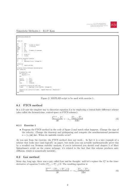
Numerische Methoden 1 – B.J.P. Kaus% advection_central_1D%clear allnx = 201;W = 40; % width of domainVel = -4; % velocitysigma = 1;Ampl = 2;nt = 500; % number of timestepsdt = 1e-2;dx = W/(nx-1);x = 0:dx:W;% Initial gaussian T-profilexc = 20;T = Ampl*exp(-(x-xc).^2/sigma^2);% VelocityVx = ones(1,nx)*Vel;% Central finite difference discretizationfor itime=1:nt% central fin. difffor ix=2:nx-1Tnew(ix) = ??endTnew(1) = T(1);Tnew(nx) = T(nx);T = Tnew;time = itime*dt;% Analytical solution for this caseT_anal = Ampl*exp(-(x-xc-time*Vel).^2/sigma^2);figure(1),clf, plot(x,T,x,T_anal),drawnowendlegend(’Numerical’,’Analytical’)Figure 2: MATLAB script to be used with exercise 1.8.1 FTCS methodIn a 1-D case the simplest way to discretize equation 3 is by employing a central finite difference scheme(also called the forward-time, central space or FTCS scheme):T n+1i− Tin∆t= −v x,iT n i+1 − T n i−12∆x(5)8.1.1 Exercise 1• Program the FTCS method in the code of figure 2 and watch what happens. Change the sign ofthe velocity. Change the timestep and gridspacing and compute the nondimensional parameterα = |v x |∆t/∆x. When do unstable results occur?As you saw from the exercise, the FTCS method does not work... In fact it is a nice example of ascheme that looks nice (and logical!) on paper, but sucks [you can actually mathematically prove thisby a socalled von Neuman stability analysis, if you’re interested you should read chapter 5 of MarcSpiegelman’s script on the course webpage; it’s related to the fact that this scheme produces antidiffusion,which is numerically instable].8.2 Lax methodin the time-Some day, long ago, there was a guy called Lax and he thought: well let’s replace the Tinderivative of equation 5 with (Ti+1 n + T i−1 n )/2. The resulting equation isT n+1i − (Ti+1 n + T i−1 n )/2 Ti+1 n = −v − T i−1nx,i∆t2∆x(6)2