Analytical Advection–Dispersion Model for Transport ... - PC-Progress

is approximately uniform with depth. Previous theoretical analysesof water flow with root uptake have found that the pressurehead depth-profile is generally very uniform during steady flow(Raats, 1974) or quasi-steady flow such as may be achieved withhigh frequency irrigation (Rawlins, 1973). Steady-state watercontent profiles computed by Yuan and Lu (2005, their Fig. 4)similarly showed a high degree of uniformity in the root zone.To further justify the uniform water content approximationinvoked above, we present in this section an analysis of steadyflow that extends the work of Raats (1974).Consider the specific case of a uniform soil where the steadywater flux is specified by the Buckingham-Darcy law, in whichcase Eq. [1] becomesd ⎡ dh⎤− K + K + rw( z) = 0[9]dz⎢ dz⎥⎣ ⎦where h is the pressure head (L) and K is the hydraulic conductivity(L T −1 ). The hydraulic conductivity is assumed to be ofthe form (Gardner, 1958)Kh ( ) Ke αh= s[10]where K s (L T −1 ) is the saturated hydraulic conductivity and α(L −1 ) is the Gardner parameter that ranges approximately from0.1 cm −1 for coarse-textured soils to 0.01 cm −1 for fine-texturedsoils (Raats, 1974). Using the root water uptake term ofRaats (1974), r w (z) is given byw ( ) ( / )e −r z Tz / δ= δ [11]Equation [11] prescribes an exponential uptake distribution,with the distribution parameter δ (L) corresponding to the depthof an equivalent uniform root system having the same uptakeand transpiration rates (Raats, 1974). Although Eq. [11] accommodatesan infinite rooting depth, 99.8% of the uptake occurswithin a depth of 6δ.For the soil surface boundary condition,dhq0= − K(0) (0) + K(0)[12]dzand the lower boundary condition at a depth z = L,⎡αΔ h= − −⎣in whichLFln 1 (1 1/ LF)⎢1q0−T≡q0αδ ⎤+αδ⎥⎦[15][16]is termed the leaching fraction (i.e., the fraction of q 0 that passesbelow the root zone).Figure 1 shows a plot of αΔh versus the dimensionlessparameter αδ for various values of L F . The limit αδ → 0 correspondsto a very fine soil and/or a shallow root distribution,whereas αδ → ∞ implies a coarse-textured soil and/or very deeprooting (Raats, 1974). Figure 1 indicates that the differencebetween the pressure head at the soil surface and at the effectivebase of the root zone is smaller (i.e., the profile becomes moreuniform) when L F is large and/or αδ is small. This means thathigh leaching fractions (large L F ), fine-textured soils (small α),and shallow rooting depths (small δ) promote uniformity in thepressure head profile.To make these generalities more quantitative, consider thatthe maximum rooting depth, R D , for common agricultural cropsranges from about 100 to 300 cm (Borg and Grimes, 1986),with the global-average value being about 210 cm (Canadell etal., 1996). Given that 99.8% of uptake occurs within a depthof 6δ, we may characterize shallow-, average-, and deep-rootedcrops as having δ = R D /6 ≈ 20, 35, and 50 cm, respectively.Among noncrop plant species, comparable global-average valuesare R D = 700 cm for trees (δ ≈ 120 cm), R D = 510 cm for shrubs(δ ≈ 85 cm), and R D = 260 cm for herbaceous plants (δ ≈ 45cm) (Canadell et al., 1996).Figure 2 shows Δh plotted versus R D (= 6δ) for fine-textured(α = 0.01 cm −1 ) and coarse-textured (α = 0.1 cm −1 ) soilsand various values of L F . For α = 0.1 cm −1 (dashed lines), Δhchanges very little as R D increases from 100 (shallow rooted crop)to 700 cm (tree), indicating that rooting depth is of lesser importancein determining pressure head uniformity in the coarse soil.The effect of the leaching fraction is more significant, with Δhincreasing approximately from 7 to 22 cm when L F is decreasedd h ( z = L)= 0dz[13]the solution of Eq. [9] for L → ∞ may be expressed as⎡q0T ⎛ αδ −z/ δ⎞⎤α hz ( ) = ln − 1− e⎢KsK ⎜s⎝1+αδ⎠⎟⎥[14]⎣⎦Raats (1974, Eq. [21]) presented an equivalent resultexpressed in terms of the matric flux potential instead of thepressure head. Equation [14] indicates that the pressure headwill decrease downward, from a high value at the soil surfacedown to some constant value as z → ∞ (or, more practically, asz → ≈6δ). Profile uniformity can be evaluated by calculating thedifference between the pressure head at the soil surface and atdepth, Δh ≡ h(0) − h(∞). From Eq. [14] it follows that this pressurehead difference is given byFIG. 1. Plot of αΔh as a function of αδ for various values of the leachingfraction, L F (α = Gardner conductivity parameter [L −1 ]; δ = Raatsuptake distribution parameter [L]; and Δh = change in pressure headbetween top and bottom of root zone [L]).www.vadosezonejournal.org · Vol. 6, No. 4, November 2007 892

FIG. 2. The change in pressure head between the top and bottom ofthe root zone (Δh) plotted as a function of rooting depth. Plots areshown for two soil types (α = Gardner conductivity parameter [L −1 ])and various values of the leaching fraction (L F ).from 0.5 to 0.1 (across rooting depths of interest, R D > 100cm). For the fine-textured soil (α = 0.01 cm −1 , solid lines), therooting depth is far more important. For example, when L F =0.3, Δh increases from 29 to 81 cm when R D is increased from100 to 700 cm. The leaching fraction is also significant for thefine-textured soil: when R D = 300 cm (deep-rooted crop), Δhincreases from 29 to 139 cm when L F is decreased from 0.5 to0.1.The largest calculated Δh values were approximately 180cm for the fine-textured soil (L F = 0.1, R D = 700 cm) and 22cm for the coarse-textured soil (L F = 0.1, R D > 100 cm). Theseresults correspond to low leaching and deep rooting scenarios,such as might be found in semiarid and arid climates. Even forthese “worst-case” scenarios, however, the variation in the watercontent may not be excessive, depending on the nonlinearity ofthe retention function, θ(h), and the magnitude of dθ/dh. Thenonlinearity in θ(h) means that the change in water content for agiven Δh will depend on the pressure head at the soil surface, h(z= 0). For fine-textured soils where dθ/dh is typically very modestlysized for all h values, a small Δh will correspond to a smallchange in water content, whereas for coarse-textured soils, dθ/dhmay become large such that a small Δh can produce a relativelylarge change in water content if h(z = 0) is in the vicinity of thesteep part of the retention curve.The water content variation can be assessed quantitativelyusing the Russo (1988) model to describe the saturation:−0.5αhSh ( ) = ⎡e (1+ 0.5 α h)⎤⎢⎣⎥⎦2/(2 + m )[17]where S is effective saturation (0 ≤ S ≤ 1) and m is Mualem’s(1976) tortuosity parameter, which we assume has the value m= 0.5. The difference in saturation between the surface and thebase of the root zone is ΔS ≡ S[h(0)] − S[h(∞)] = S[h(0)] − S[h(0)− Δh]. Figure 3 shows plots of ΔS as a function of h(0). Theseplots were made using the leaching fraction and root depth combinationsthat produced the largest and smallest values of Δhobserved in Fig. 2 (where R D ≥ 100 cm). Thus, the water contentvariations shown in Fig. 3 correspond to the greatest- and leastuniformpressure head profiles plotted in Fig. 2. As expected,Fig. 3 demonstrates that in addition to the aforementionedeffects of rooting depth and leaching fraction, the uniformity ofthe soil water content profile is affected by the pressure head (orwater content) at the soil surface. In evaluating Fig. 3, our experiencesuggests that when ΔS is less than about 0.1, the watercontent variability can be safely treated as negligible since thatlevel of variability is similar to the precision that is obtainablewith, for example, electromagnetic methods of measuring watercontents under field conditions. While it is not possible to stateprecisely the general conditions for which an effective, uniformwater content approximation is acceptable, we conclude that theapproximation is reasonable whenever the leaching fraction issufficiently large (e.g., ≥0.25). For coarse-textured soils wheredθ/dh is large near the wet end of the retention curve, there is anadditional requirement that the soil surface be drier than wherethe steep part of the curve is located (for the coarse soil depictedin Fig. 2, h(z = 0) must be less than approximately −75 cm).Thus far, this section has been concerned with the internalconsistency of the proposed transport model. That is, we haveaddressed the question of whether the water content can be reasonablyapproximated as uniform given the model assumptionsof uniform soil properties and steady flow. Once that questionis resolved, a related but separate question that may be asked iswhether a model that specifies a uniform water content can beused to assess transport in fields where the water content is clearlynonuniform (e.g., in layered soil profiles). Evidence exists (e.g.,Wierenga, 1977; Streck and Piehler, 1998) that solute distributionsmodeled using an effective uniform water content are notsignificantly different from those modeled using an explicit representationof the water content variability. Thus, we concludethat Eq. [8] may be useful in the case of nonuniform soil profilesif an appropriate effective water content can be determined.First-Order Plant UptakeThe proposed transport model assumes that solute uptakeis a first-order process (Eq. [7]). The plant uptake of solutes isFIG. 3. Changes in soil water saturation between the top and bottomof the root zone (ΔS) plotted as a function of the soil surface pressurehead for two soil types. Plots are shown for a low-leaching,deep-rooting scenario and a high-leaching, shallow-rooting scenario.(α = Gardner conductivity parameter; L F = leaching fraction; R D =maximum rooting depth; Δh = difference in pressure head betweenthe top and bottom of root zone; h = pressure head; and z = depth.)www.vadosezonejournal.org · Vol. 6, No. 4, November 2007 893

a highly complex process that depends on plant species, solutespecies, and solution composition (e.g., the uptake of cadmiumis affected by the presence of other divalent cations) (Tinkerand Nye, 2000). Detailed, mechanistic descriptions of uptake–absorption processes are possible, but these defy a simple mathematicaldescription. Measurements of uptake kinetics commonlyshow that uptake increases linearly with solution concentrationat low concentrations and then levels off and becomes constantat high concentrations. Consistent with these observations,uptake is often modeled assuming Michaelis-Menten kinetics(Tinker and Nye, 2000):Crs∝[18]K + CMwhere K M is the Michaelis–Menten constant. Alternatively,uptake may be modeled using two intersecting lines (Tinkerand Nye, 2000), one representing a linear increase in uptakebelow some critical or threshold concentration, and one representinga constant maximum uptake rate above the criticalconcentration (Fig. 4).When the concentration remains below the threshold concentration,the first-order uptake model is consistent with thetwo-line model, with the uptake coefficient γ being proportionalto the slope of the first line segment (Fig. 4). A connection withthe Michaelis–Menten representation also exists at low concentrations(K M >> C), where the Michaelis–Menten model maybe approximated as r s ∝ C/K M . In this case, the uptake coefficientis γ ∝ 1/K M . Note that if γ is related to K M in this way,then uptake calculated for a given concentration with Eq. [7]will always be greater than or equal to that specified by the correspondingMichaelis–Menten model (Fig. 4).Analytical SolutionWe define D 0 ≡ D(z = 0) and consider the solution of Eq.[8] subject to the following boundary and initial conditions⎛= ⎜ −∂C⎞⎟vC 0 0 vC 0 D0z ⎝⎜ ∂ ⎠⎟z=0∂C ( Lt , ) = 0∂z[19][20]Cz ( ,0)= C[21]Iwhere C 0 is the concentration of the infiltrating solution and C Iis the initial concentration of the soil water. An analytical solutionmay be obtained using the generalized integral transformtechnique, or GITT (Ozisik and Murray, 1974; Cotta, 1993;Liu et al., 2000). Liu et al. (2000) reported the GITT solutionof a generic transport equation of which Eq. [8] is a special case.For the present problem, the solution given by Liu et al. (2000)may be written as0M1/2∑ n n n[22]n=1Czt ( , ) = C + N ϕ ( zT ) ( t)where the infinite summation required in the formal solutionhas been truncated at M terms and where the eigenfunction ϕ nand its norm N n are, respectively,ϕ n( z) = cos[ βn( L− z)][23]Nn1 ⎛ vD= L+2⎜⎝β +0 02 2 2nD0 v0⎞ ⎠⎟The eigenvalues β n are the first M zeros of the equation0 n 0 n n[24]v cos( β L) −D β sin( β L) = 0[25]Because of the specific form of Eq. [8] and the boundary conditionsimposed, it is possible to simplify the expression presentedby Liu et al. (2000) for T n (t). Letting T(t) be a M-length vectorwith nth element T n (t), values for T n (t) in Eq. [22] can beobtained by computing (cf. Liu et al., 2000, Eq. [13])−1 −1 −1T( t) = exp( −A Bt)[ T(0) − B G]+ B G[26]where elements of the M × M matrices A and B and the M-length vectors G and T(0) are given by− 1/2 −1/2Lnr = n r ϕ0n ϕrA N N ∫ R ( z) ( z)dz[27]−1/2 −1/2⎧⎪ Ld ϕr( z )Bnr = Nn N ⎪r ⎨ [ v00 −vT B( z)] ϕn( z) dz⎪∫⎪⎩dzL d ϕr( z)d ϕn( z)+ ∫ Dz ( ) dz0 dzdz∫− (1 −γ) v b( z) ϕ ( z) ϕ ( z)d z+ v ϕ (0) ϕ (0)0LT n r 0 r n}[28]−1/2Ln = 0 n −γ0T ϕnG C N ∫ (1 ) v b( z) ( z)dz[29]−1/2n(0) ( I 0) n sin( n)/nT = C −C N Lβ β [30]FIG. 4. Illustration of the Michaelis–Menten and two-line uptakemodels. Also shown is a dilute solution approximation of the Michaelis–Mentenmodel.A computer program implementing the presented solution isavailable from the senior author. For simplicity we consideredin this study a constant inlet concentration, C 0 (t) = C 0 , and aconstant initial concentration, C I (z) = C I . A solution for the caseof a time-varying inlet and depth-varying initial concentrationcan also be obtained, although in that case the computation ofT n is more complicated due to the time dependence of G n (seeLiu et al., 2000).www.vadosezonejournal.org · Vol. 6, No. 4, November 2007 894

It is also of interest to consider the steady-state (∂C/∂t = 0)solution of the transport equation (Eq. [8]) for the special caseof no dispersion (D = 0). In this case, a solution can be obtainedby separation-of-variables, with the result being1−γ⎡ 1 ⎤Cz ( )/ C0= ⎢ 1 −(1 −LF) B( z)⎥[31]⎣⎦where the leaching fraction is defined as before, that is, L F = (v 0− v T )/v 0 = (q 0 − T)/q 0 .Results and DiscussionGeneral Model CharacteristicsFigures 5 and 6 contain plots that illustrate general characteristicsof the advection–dispersion model with uptake of waterand solute. The scenarios depicted in these figures involve, beginningat time t = 0 d, the application of water with solute concentrationC 0 to a soil that has an initially uniform concentration ofC I = 0.25 C 0 . The solid lines in the plots are concentration vs.depth profiles computed with the analytical solution presentedin the previous section (Eq. [22]). The dashed lines are steadystateprofiles computed with Eq. [31] for D = 0. The simulationsassume an exponential water uptake distribution (Eq. [11]) anda dispersion coefficient that was specified asFigure 5 shows concentration profiles computed for successivetimes. At very early times (5 d, in this example), the soluteprofile is qualitatively similar to that predicted with standardadvection–dispersion models. The similarity ends quickly,however, as the concentration behind the front becomes largerthan C 0 while the leading edge retains the familiar dispersiveshape. This solute build-up is due to the concentrating effects ofa water flux that decreases with depth. At later times the soluteprofile reaches a steady state, with solute concentrations increasingfrom a minimal value at the soil surface to a maximal valueat and below the base of the root zone. The maximum concentrationthat will be achieved is a function of the amount ofwater and solute being taken up, as determined by the leachingfraction (L F ) and the solute uptake coefficient (γ). When γ ≠ 0,the maximum concentration is also affected by the value of thedispersion coefficient.Figure 6 illustrates the effects of the uptake coefficient (γ)and dispersivity (α L ) on the solute profile. The profiles shown assolid lines are for a large time value such that solute concentrationswithin the root zone (z ≤ 6δ) have obtained approximatelyDz ( ) = α vz ( ) = α [ v − v Bz ( )][32]L L 0 Twhere α L is the dispersivity (L). Model and algorithm parametervalues are given in the figure captions. Note that the computationaldomain length L was much larger than the plotted depthsuch that the plotted results are for an effectively semi-infiniteprofile. Also, for simplicity we assumed a value of R = 1 for theretardation factor; using a larger R value merely shifts the plotsto later times.FIG. 5. Plots of solute concentration vs. depth computed for successivetimes with the advection–dispersion transport model. Theconcentration profi les were computed using the following parametervalues: R = 1, δ = 20 cm, v 0 = 1 cm d −1 , v T = 0.75 cm d −1 , γ = 0.1,α L = 10 cm, C I = 0.25 C 0 , L = 1000 cm, and M = 80. Dashed lines aresteady-state results computed for D = 0. (R = retardation factor; δ =root distribution parameter; q 0 = water fl ux at soil surface; T = transpirationrate; θ = volumetric water content; v 0 ≡ q 0 /θ; v T ≡ T/θ; γ =fi rst-order solute uptake coeffi cient; α L = dispersivity; D = dispersioncoeffi cient; C I = initial soil solution concentration; C 0 = infi ltrating solutionconcentration; L = depth of computational domain; M = numberof terms summed in analytical solution.)FIG. 6. Plots of solute concentration vs. depth computed for variousvalues of the transport parameters γ and α L . Except where indicatedotherwise, the concentration profi les were computed using the followingparameter values: t = 1000 d, R = 1, δ = 20 cm, v 0 = 1 cm d −1 ,v T = 0.75 cm d −1 , γ = 0.1, α L = 10 cm, C I = 0.25 C 0 , L = 1000 cm,and M = 80. Dashed lines are steady-state results computed for D= 0. (t = time; R = retardation factor; δ = root distribution parameter;q 0 = water fl ux at soil surface; T = transpiration rate; θ = volumetricwater content; v 0 ≡ q 0 /θ; v T ≡ T/θ; γ = fi rst-order solute uptake coefficient; α L = dispersivity; D = dispersion coeffi cient; C I = initial soilsolution concentration; C 0 = infi ltrating solution concentration; L =depth of computational domain; M = number of terms summed inanalytical solution.)www.vadosezonejournal.org · Vol. 6, No. 4, November 2007 895

their steady values, whereas concentrations a short distancebelow the root zone are still increasing. Figure 6a shows thatwhen no solute is excluded from the uptake process (γ = 1), rootzone solute concentrations do not increase above C 0 ; the steadystateprofile is simply C(z) = C 0 . For γ = 0, no solute is takenup by the roots and the build-up of solute is maximized. Alsoshown is the result for the intermediate case γ = 0.5. For γ = 1.5,active uptake of solute occurs. In this particular case the steadysolute concentration profile decreases with depth, approaching aconstant value that is less than C 0 but greater than C I .Figure 6b illustrates the effects of dispersion on solute profiledevelopment. The profiles were computed for three valuesof the dispersivity: 2, 10, and 30 cm. As expected, the resultsshow that increasing the value of the dispersivity produces moresolute spreading at the front, which increases the time requiredfor the profile to reach steady state: the α L = 2 cm profile at t =1000 d has very nearly reached steady state, whereas the α L = 30cm profile is still increasing in the bottom of the root zone. Alsoas expected, the computed solute profile approaches the steadystate,D = 0 solution (dashed line, Eq. [31]) as the dispersivityapproaches zero.The computed profiles in Fig. 6b also illustrate a possiblelimitation of the advection–dispersion model as applied to transportwith simultaneous water and solute uptake. The problem isthat when solute builds up in the root zone, a positive concentrationgradient develops (i.e., directed back toward the soil surface),which, according to the advection–dispersion model, producesan accompanying diffusive–dispersive flux back toward the soilsurface. The magnitude of this flux in reality should reflect onlydiffusive processes rather than field-scale dispersion processes.The use of a diffusion–dispersion coefficient value that reflectsfield-scale dispersion processes hence causes an excessively largeupward component of the solute flux, leading to near-surfaceroot zone concentrations that are too large. The higher the dispersivity,the more the surface concentration will exceed C 0 . Thefield-scale dispersivity typically has a value in the range of 5 to20 cm (Jury et al., 1991), although this parameter often carriesa high degree of uncertainty. Given this uncertainty and thepossible limitations of the advection–dispersion model, it wouldseem prudent to err on the side of choosing a relatively smallvalue of α L (or D) when using this model. This limitation is notexclusive to the model developed here; the same considerationsshould apply to any advection–dispersion model that featuresroot uptake, such as the comprehensive numerical models notedin the introduction.Example ApplicationCadmium is one of the most mobile and bioavailable tracemetals and constitutes a potential human health risk throughdietary intake (Buchet et al., 1990). In many locations the cadmiumcontent of arable soils has significantly increased overthe years, primarily from application of cadmium-containingphosphorous fertilizers and from atmospheric deposition. Thecadmium content in Swedish arable soils, for example, hasapparently increased by about 30% since the beginning of thetwentieth century (Andersson, 1992). The current soil contentof cadmium can result in concentrations in harvested plant partsthat are close to acceptable limits set for human consumption inmany countries (e.g., Eriksson et al., 2000).Legislative standards for allowable or critical metal loadingsto arable land vary by country. One emerging method for riskassessment involves simple mass balance calculations whereinthe soil is treated as a single compartment subject to first-orderuptake into harvested plant parts, linear sorption partitioningin the soil, and advective leaching below the root zone (Pačes,1998; Tiktak et al., 1998; Blombäck et al., 2000; Bergkvist et al.,2005). Such an approach implicitly assumes uniform well-mixedconditions within the soil compartment and ignores depth variationsof transport and uptake of both water and trace metalsin the root zone. Given these assumptions, and using the samenotation as above, the change in stored amount A (M L −2 ) isgiven bydA = qC 0 0− qC z −γ TC[33]dtwhere q z is the water flow at the base of the root zone and A = (θ+ ρ b K d )R d C. Noting that q z = q 0 – T leads todC= I− kC[34]dtwhere I = (v 0 C 0 )/(RR D ) and k = [v 0 + v T (γ − 1)]/(RR D ). WhenC(0) = C I , integrating Eq. [34] from t = 0 to t gives⎛I⎞ −ktCt () = ⎜ ( 1− e ) + CIe⎜⎝k⎠⎟−kt[35]In the one-compartment model, the concentration of harvestedparts of annual plants C p (M m −1 ) is given byγTCCp()t = [36]Bpwhere B p is the harvested biomass yield (M L −2 T −1 ). Thisexpression is appropriate only for plants whose growth cycle isshort relative to the timescale of solute transport in the root zone(e.g., annual crops). Setting dC/dt = 0 in the one-compartmentmodel gives the steady-state soil solution concentration asC0C = [37]1 + ( γ− 1 )(1 − LF)and the steady-state plant concentration asγTC0C P =[38]Bp[1+ ( γ−1 )(1 −LF)]In our example application, we compare the analyticaladvection–dispersion and one-compartment models for the caseof cadmium uptake into wheat grain, an important staple foodin many parts of the world. The advection–dispersion model inthis example was implemented using a constant dispersion coefficient,D(z) = D, and a linear uptake distribution,bz ( )⎧⎪ 0.8 1.6⎪− z z ≤R2= ⎨RDR ⎪⎪D0 z >⎪⎩RDD[39]This uptake distribution conforms to the “40:30:20:10 rule”(e.g., Raats, 1974; Hoffman and van Genuchten, 1983), suchthat 40% of the uptake is in the top quarter of the root zone,30% in the second quarter, 20% in the third quarter, and 10%in the bottom quarter. Omitting details, an expression equiva-www.vadosezonejournal.org · Vol. 6, No. 4, November 2007 896

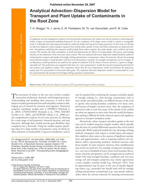
lent to Eq. [36] may be developed for the advection–dispersionmodel to compute the harvested plant part concentration:1 1CP() t = r d z = γTb( z) C(,)dz t zBPRDRD0sBP0∫ ∫ [40]The uptake coefficient γ is an important parameter since itdetermines the extent to which cadmium in the soil solution isexcluded from the plant. Measurements of cadmium uptake haveindicated that uptake is linear over a range of concentrationsrelevant for sludge applications (Hamon et al., 1999; McGrathet al., 2000). Measurements of cadmium concentrations in soilsolutions and wheat grain (Bergkvist et al., 2005), together withtypical values of the water use efficiency T/B p for wheat (see Eq.[36]), suggest a value for γ of approximately 0.05, which we usedin the calculations presented below. The remaining parametervalues are shown in the caption of Fig. 7, which compares predictionsof the two models. The assumed cadmium loading rate(1.6 mg m −2 yr −1 ) reflects all sources of cadmium. In the wheatgrowingareas of Europe, diffuse aerial deposition, together withimpurities in lime, commercial fertilizer, and feeds, would notsupply more than approximately 0.3 to 0.5 mg Cd m −2 yr −1 .Thus, for the scenario depicted in Fig. 7, we implicitly assumea significant additional local cadmium source such as industrialemissions or sludge applications. The assumed loading rate isnot unrealistic in that the current allowable limit in the EU forcadmium supplied with sludge is set at 15 mg m −2 yr −1 (EUdirective, 86/278/EEC).Figure 7 shows that for the above parameterization, theanalytical advection–dispersion model predicts a final steadystateCd concentration in wheat grain of approximately 0.2 mgkg −1 , reached after about 500 yr, which equals the allowableconcentration under EU directives. The root depth in the onecompartmentmodel is usually set to the plow depth (?0.25 m)since this best approximates the assumption of uniform mixing(e.g., Tiktak et al., 1998). This assumption ignores subsoiluptake of cadmium, which can be considerable (Johnsson et al.,2002). Figure 7 shows that with R D = 0.25 m, the one-compartmentmodel substantially overestimates the grain cadmiumconcentration, although the pattern of increase is similar to theanalytical advection–dispersion model, with a steady-state valueapproached after approximately 500 yr. Increasing R D to 1 m, tomatch the maximum depth of roots in the advection–dispersionmodel, produces good agreement with the advection–dispersionmodel at early times (up to 300 yr). However, the final steadystatevalue of the one-compartment model is independent of R D(see Eq. [38]), being about 75% larger than the value predictedby the advection–dispersion model. In terms of risk assessment,such a difference in model results is highly significant. We concludethat the simplifications in the one-compartment modelcan lead to erroneous decisions, although the predicted deviationsin the present example would become significant only aftera few hundred years depending on the value of R D used in theone-compartment model. Finally, we note that the analyticaladvection–dispersion model requires only a few extra parameters,which are easily estimated. The advection–dispersion modeltherefore should be recommended as the preferred tool for environmentalrisk assessment of persistent contaminants.ConclusionsAlthough a variety of comprehensive numerical simulationmodels exist for analyzing solute transport processes in the rootzone, regulatory and risk management analyses often requiresimpler modeling tools with fewer input parameters. Simpleranalytical models may be especially useful for assessing environmentalimpacts of strongly sorbing and persistent solutes suchas trace metals. This is because the relevant timescales for suchassessments are measured in decades or centuries, in which casetransport and plant uptake can be modeled effectively usingannual and root-zone average parameters.In this work we developed an analytical advection–dispersionmodel that includes plant uptake of water and solute.Although considerably simpler than many popular comprehensivenumerical models, the analytical advection–dispersionmodel—with its explicit accounting of advection, dispersion,and uptake processes within the root zone—is much more realisticthan one-compartment, well-mixed models that are currentlybeing used or considered for use in risk assessments. As an example,we compared predictions made with the advection–dispersionand one-compartment models for the uptake of cadmiumby wheat. The comparison showed that the one-compartmentmodel significantly overestimated the long-term, steady-stateCd concentration in harvested wheat grain. For this reason, werecommend the analytical advection–dispersion model as a preferredtool for environmental risk assessment of strongly sorbing,persistent solutes.Possible limitations of the presented model arise due toassumptions of linear solute sorption and first-order plantuptake. We thus suggest that model applications be restrictedto cases of slight to moderate soil contamination where theseassumptions are likely to be reasonable. Additionally, the modelFIG. 7. A comparison of predictions of the analytical advection-dispersionand one-compartment models for cadmium uptake into wheatgrain using the following parameter values: q 0 = 0.7 m yr −1 , T = 0.5m yr −1 , γ = 0.05, B p = 0.5 kg m −2 yr −1 , θ = 0.4 m 3 m −3 , R = 376, D= 0.015 m 2 yr −1 , C I = 1 mg m −3 and C 0 = 2.286 mg m −3 , equivalentto a cadmium loading of 1.6 mg m −2 yr −1 . The root depth, R D , in theadvection–dispersion equation model was set to 1 m, and two valuesof R D are shown for the one-compartment model (0.25 and 1 m). (q 0= water fl ux at soil surface; T = transpiration rate; γ = first-order soluteuptake coeffi cient; B p = harvested biomass yield; θ = volumetricwater content; R = retardation factor; D = dispersion coeffi cient; C I =initial soil solution concentration; C 0 = infi ltrating solution concentration;R D = maximum rooting depth.)www.vadosezonejournal.org · Vol. 6, No. 4, November 2007 897

was derived based on an assumption of uniform soil water content.Among other factors, water content uniformity is affectedby soil texture, rooting depth, and leaching fraction, with finetexture, shallow rooting, and high leaching all promoting uniformity.In general, a leaching fraction of greater than about 0.25corresponds to a fairly uniform profile when steady-state waterflow occurs, except perhaps in very coarse-textured soils wheresubstantial nonuniformity could arise if the surface soil were tobe maintained at a high degree of saturation. Where nonuniformsoil conditions prevail, the model may be used if an appropriate,effective water content can be identified.ACKNOWLEDGMENTSThis research was supported in part by the Swedish EnvironmentalProtection Agency funded project “Cadmium leaching from arable landand uptake into crops: calculation of critical loads and developmentof a simulation tool for dynamic long-term predictions”; a fellowshipfrom CNPq (Brazil) to E. M. Pontedeiro; and the SAHRA Science andTechnology Center as part of NSF grant EAR-9876800.ReferencesAhuja, L.R., K.W. Rojas, J.D. Hanson, M.J. Shaffer, and L. Ma (ed.). 2000. Rootzone water quality model: Modeling management effects on water qualityand crop production. Water Resources Publications, LLC, HighlandsRanch, CO.Andersson, A. 1992. Trace elements in agricultural soils: Fluxes, balances, andbackground values. Report 4077. Swedish Environmental ProtectionAgency, Solna.Bergkvist, P., N.J. Jarvis, J. Eriksson, and L. Rapp. 2005. Critical load of cadmiumon arable soils in Sweden. Emergo no. 4, Studies in the BiogeophysicalEnvironment. Dep. of Soil Sci., Swedish Univ. of Agricultural Sciences,Uppsala.Blombäck, K., M. Kalvi, J. Eriksson, and I. Öborn. 2000. Cadmium accumulationin agricultural soils and uptake by plants as an effect of cadmium inphosphate fertilizers: Model estimations. p. 11–31. In Assessment of risksto health and the environment in Sweden from cadmium in fertilizers.Report 4/00. National Chemicals Inspectorate, Stockholm.Borg, H., and D.W. Grimes. 1986. Depth development of roots with time: Anempirical description. Trans. ASAE 29:194–197.Buchet, J.P., R. Lauwerys, H. Roels, A. Bernard, P. Bruaux, F. Claeys, G.Ducoffre, P. de Plaen, J. Staessen, A. Amery, P. Lijnen, L. Thijs, D. Rondia,F. Sartor, A. Saint Remy, and L. Nick. 1990. Renal effects of cadmiumbody burden of the general population. Lancet 336:699–702.Canadell, J., R.B. Jackson, J.R. Ehleringer, H.A. Mooney, O.E. Sala, and E.-D.Schulze. 1996. Maximum rooting depth of vegetation types at the globalscale. Oecologia 108:583–595.Cotta, R.M. 1993. Integral transforms in computational heat and fluid flow.CRC Press, Boca Raton, FL.Dalton, F.N., P.A.C. Raats, and W.R. Gardner. 1975. Simultaneous uptake ofwater and solutes by plant roots. Agron. J. 67:334–339.Destouni, G. 1991. Applicability of the steady state flow assumption for soluteadvection in field soils. Water Resour. Res. 27:2129–2140.Eriksson, J., A. Andersson, B. Stenberg, and R. Andersson. 2000. Current statusof Swedish arable soils and cereals. Report 5062. (Summary in English.)Swedish Environmental Protection Agency, Stockholm.Feddes, R.A., P.J. Kowalik, and H. Zaradny. 1978. Simulation of field water useand crop yield. PUDOC, Wageningen, the Netherlands.Gardner, W.R. 1958. Some steady-state solutions of the unsaturated moistureflow equation with application to evaporation from a water table. Soil Sci.85:228–232.Ginn, T.R., and E.M. Murphy. 1997. A transient flux model for convectiveinfiltration: Forward and inverse solutions for chloride mass balancestudies. Water Resour. Res. 33:2065–2079.Hamon, R.E., P.E. Holm, S.E. Lorenz, S.P. McGrath, and T.H. Christensen.1999. Metal uptake by plants from sludge-amended soils: Caution isrequired in the plateau interpretation. Plant Soil 216:53–64.Hoffman, G.J., and M.Th. van Genuchten. 1983. Soil properties and efficientwater use: Water management for salinity control. p. 73–85. In H.M.Taylor, W.R. Jordan, and T.R. Sinclair (ed.) Limitations to efficient wateruse in crop production. ASA, CSSA, and SSSA, Madison, WI.Johnsson, L., I. Öborn, G. Jansson, and D. Berggren. 2002. Evidence for springwheat (Triticum aestivum) uptake from subsurface soils. In Y. Zhu and Y.Tong (ed.) Proc. of the Int. Workshop of Soil-Plant Interactions, Beijing,China. 27–30 Oct. 2002. Kluwer Academic, Dordrecht, the Netherlands.Jury, W.A., W.R. Gardner, and W.H. Gardner. 1991. Soil physics. John Wiley& Sons, New York.Larsbo, M., S. Roulier, F. Stenemo, R. Kasteel, and N.J. Jarvis. 2005. Animproved dual-permeability model of water flow and solute transport inthe vadose zone. Vadose Zone J. 4:398–406.Liu, C., J.E. Szecsody, J.M. Zachara, and W.P. Ball. 2000. Use of the generalizedintegral transform method for solving equations of solute transport inporous media. Adv. Water Resour. 23:483–492.McGrath, S.P., F.J. Zhao, S.J. Dunham, A.R. Crosland, and K. Coleman. 2000.Long-term changes in the extractability and bioavailability of zinc andcadmium after sludge application. J. Environ. Qual. 29:875–882.Mualem, Y. 1976. A new model for predicting the hydraulic conductivity ofunsaturated porous media. Water Resour. Res. 12:513–522.Ozisik, M.N., and R.L. Murray. 1974. On the solution of linear diffusionproblems with variable boundary condition parameters. J. Heat Transfer96:48–51.Pačes, T. 1998. Critical loads of trace metals in soils: A method of calculation.Water Air Soil Pollut. 105:451–458.Raats, P.A.C. 1974. Steady flows of water and salt in uniform soil profiles withplant roots. Soil Sci. Soc. Am. Proc. 38:717–722.Raats, P.A.C. 1975. Distributions of salts in the root zone. J. Hydrol. 27:237–248.Raats, P.A.C. 1981. Residence times of water and solutes within and below theroot zone. Agric. Water Manage. 4:63–82.Rawlins, S.L. 1973. Principles of managing high frequency irrigation. Soil Sci.Soc. Am. Proc. 37:626–629.Russo, D. 1988. Determining soil hydraulic properties by parameter estimation:On the selection of a model for the hydraulic properties. Water Resour.Res. 24:453–459.Schoups, G., and J.W. Hopmans. 2002. Analytical model for vadose zone solutetransport with root water and solute uptake. Vadose Zone J. 1:158–171.Šimůnek, J., D.L. Suarez, and M. Šejna. 1996. The UNSATCHEM softwarepackage for simulating one-dimensional variably saturated water flow, heattransport, carbon dioxide production and transport, and multicomponentsolute transport with major ion equilibrium and kinetic chemistry, Version2.0. Res. Rep. no. 141. U.S. Salinity Lab., Riverside, CA.Šimůnek, J., M.Th. van Genuchten, and M. Šejna. 2005. The HYDRUS-1D software package for simulating the one-dimensional movementof water, heat and multiple solutes in variably-saturated media, Version3.0. HYDRUS Software Ser. no. 1. Dep. of Environ. Sci., Univ. of Calif.,Riverside.Skaggs, T.H., and F.J. Leij. 2002. Solute transport: Theoretical background. p.1353–1380. In J. Dane and C. Topp (ed.) Methods of soil analysis. Part 4.ASA and SSSA, Madison, WI.Skaggs, T.H., M.Th. van Genuchten, P.J. Shouse, and J.A. Poss. 2006.Macroscopic approaches to root water uptake as a function of water andsalinity stress. Agric. Water Manage. 86:140–149.Streck, T., and H. Piehler. 1998. On field-scale dispersion of strongly sorbingsolutes in soils. Water Resour. Res. 34:2769–2773.Tiktak, A., R. Alkemade, H. van Grinsven, and K. Makaske. 1998. Modelingcadmium accumulation at a regional scale in the Netherlands. Nutr.Cycling Agroecosyst. 50:209–222.Tinker, P.B., and P.H. Nye. 2000. Solute movement in the rhizosphere. OxfordUniv. Press, New York.van Genuchten, M.Th., and W.J. Alves. 1982. Analytical solutions of the onedimensionalconvective-dispersive solute transport equation. USDA Tech.Bull. 1661. U.S. Gov. Print. Office, Washington, DC.Wierenga, P.J. 1977. Solute distribution profiles computed with steady-state andtransient water movement models. Soil Sci. Soc. Am. J. 41:1050–1055.Yuan, F., and Z. Lu. 2005. Analytical solutions for vertical flow in unsaturated,rooted soils with variable surface fluxes. Vadose Zone J. 4:1210–1218.www.vadosezonejournal.org · Vol. 6, No. 4, November 2007 898