Lec-6 Optsim(Fawad)(5-04-2007).pdf - Dr. SMH Zaidi - Home Page

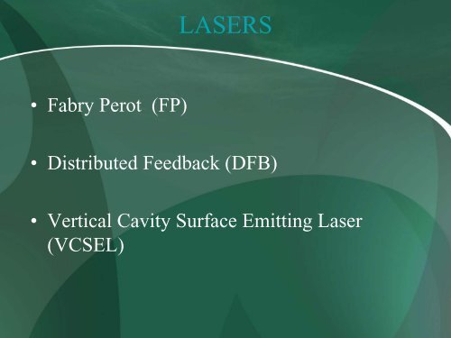
Peak Freq.• Peak Frequency = 229.644 THz [1310nm]• It can be inferred from the spectrum that spectralwidth of a FP is quite broad [~1.7 THz]

DFBSourceOpticalProbe

Peak Freq.• Peak Frequency = 228.879 THz [1310 nm]• Line width of a DFB Laser is narrower[~0.07THz]as compared to FP Laser which makes itsuitable for long haul communications

VCSELSourceOpticalProbe

Peak Freq.• Peak Frequency = 370.114 THz• Line width of a VCSEL is better than the two.[~0.04 THz] Because of low power it is suitable forshort haul communications

OptsimPresented by: Fawad Khan

What is Optsim?

Optsim Simulation SoftwareUsed to design and optimize:- DWDM and CWDM amplifiedsystems- FTTX/PON systems- OTDM systems- CATV digital/analog systems- Optical LANs- Ultra long-haul terrestrial andsubmarine systems

Motivation• Since mid-90’s, computer simulations have beenused to realistically model optical communicationsystems• Computer-aided design techniques if usedappropriately1. optimize entire system2. provide optimum values of system parameters3. Design goals are met with minimal time and cost• Commercially available design software packages- Optiwave, VPITransmission Maker, Optnet,ZeMax

Optsim Methodology• Optsim uses block-orientatedsimulation methodology in whicheach block models a component orsubsystem• Each block model is presentedgraphically as an icon, has own set ofparameters which can be modified byuser

Simulation ApproachesOptsim supports two simulationengines:1. Block mode simulation engine: signaldata is represented as one block ofdata and is passed between block toblock2. Sample mode simulation engine:signal data is represented as singlesample that is passed between blockto block

2 Simulation Modes

Simulation StepsFive steps to setting up a simulation ofa communication system:1. Create Optsim project and setsimulation parameters (Block modeVs Sample mode)2. Draw the schematic diagram3. Set parameter values of blockmodels4. Run simulation5. View results with data display tools

Modeling Stages• Stage 1: General Model (Modelingpreliminaries)• Stage 2: Select optimum parameters(Performance Evaluation)• Stage 3: See results after simulation(Optsim Validation)

Stage 1 - General Model• Design of optical communicationsystems involves optimizing a largenumber of parameters such as:• Transmitters, optical fibers,amplifiers, receivers• MUX/DEMUX, optical filters,• Optical cross connects, optical adddrop multiplexers etc

Stage 2 - Select Optimum Parameters• We need to know what type of noise is present andhow to eliminate or reduce its impact• BetterSNR (BER) should be accomplished• Attenuation minima at 1550nm• Transmitter noise could be handled by using filters• Quantum noise in case of photodiodes

Running the Simulation

Stage 3 - Optsim Validation• OptSim features performance analysis:• For example Q value• BER (Bit error rate)• Eye opening/closure• Spectrum Analyzer• Signal Analyzer• MultimeterAnalysis Tools

Case Study

Optsim View Layouts

Case Study• Take the example of a simpletransmission system with followingspecs:– Tx (Laser)– Modulator– Transmission Media (Fiber)– Rx (Photodiode)– Performance Analyzer Tool (BER Tester)

Step 1:Create Project in Block Mode

Step 2: Design Model/Schematic

Components• PRBS Generator• Electrical Generator• CW Laser• External Modulator• Fiber• ReceiverPlotting Components• BER Tester

Step 3: Select Parameters• Laser– Output Power = 4.7 dBm (Approx)– Wavelength = 1480 nm– Linewidth = 0.1nm• Fiber– Length = 10Km– Loss / km = 0.25 dB• Receiver– Quantum Efficiency = 0.85

Step 4: Run the Simulation

Step 5: View Results/ValidateRUN# BER BER_lo BER_hi1 8.8266e-055 1.2298e-059 3.8846e-050After viewing the output using BER Tester we found out that8.826e-55 is very good result

Thank You!