Scheller and Mladenoff (PDF) - Forest Landscape Ecology Lab ...

More documents

Recommendations

Info

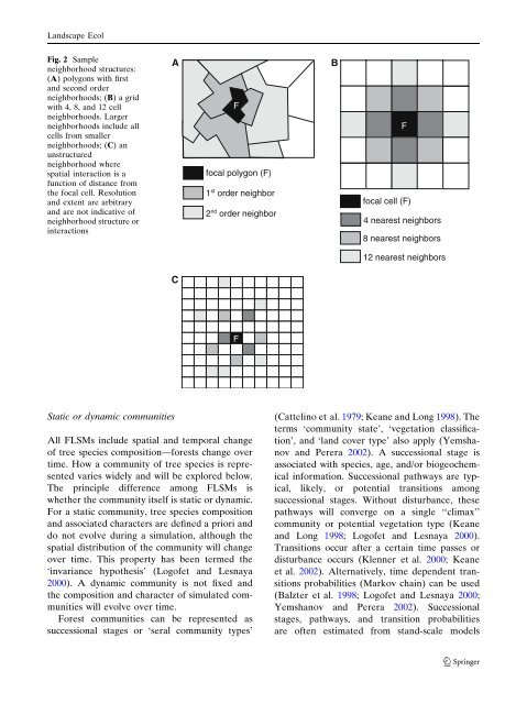
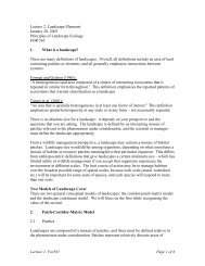
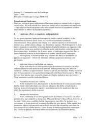
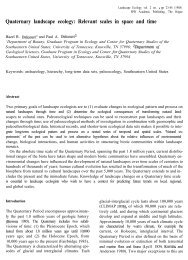
Landscape EcolForest Landscape Simulation Modelsexcluding spatialinteractionsincluding spatialinteractionsstaticcommunitiesdynamiccommunitiesstaticcommunitiesdynamiccommunitiesexcludingecosystemprocessesincludingecosystemprocessesexcludingecosystemprocessesGroup 1 Group 2 Group 3DOLY 2 TEM-LPJ 5MAPSS 1,2 IBIS 3 NoneBIOME2 2 MC1 4includingecosystemprocessesexcludingecosystemprocessesincludingecosystemprocessesexcludingecosystemprocessesincludingecosystemprocessesGroup 4 Group 5 Group 6 Group 7 Group 8ForClim 7 TELSA 8 MC1 4 LANDIS 13 FIRE-BGC 16EMBYR 10HARVEST 9MetaFor 14 LANDIS-II 17LINKAGES 6 VDDT/ SEM-LAND 11 LANDSIM 12 FACET 15Fig. 1 An example decision tree based on three ecologicalcriteria: inclusion of spatial interactions, static or dynamiccommunities, and inclusion of ecosystem processes. Theorder of the decision tree can be reconfigured, dependentupon the individual’s ranking of the three criteria. Groupnumbers correspond to the group labels in the text. Two orthree exemplar models are provided for each group.Subscripts.1 Neilson (1995);2 VEMAP Members (1995);3 Foley et al. (1996); 4 Bachelet et al. (2001a, b); 5 Pan et al.(2002);6 Pastor and Post (1986a);7 Bugmann (1996);8 Klenner et al. (2000);9 Gustafson and Crow (1998);10 Hargrove et al. (2000); 11 Li (2000); 12 Roberts (1996b);13 Mladenoff et al. (1996); 14 Urban et al. (1999); 15 Urbanand Shugart (1992); 16 Keane et al. (1996); 17 Scheller et al.(in review)patterning at multiple scales and thereforecontribute to the evolution of landscape patternand changes in spatial heterogeneity. Examplesof spatial interactions include the dispersalof seeds, a fire spreading, the movement ofherbivores, and neighboring trees competing forlight.Essential to the simulation of spatial interactionsis the representation of spatial informationand the neighborhood structure. Vector polygonsare contiguous areas that can have any size orshape within the maximum extent of the landscape(Fig. 2A). Vector polygons assume withinpolygonhomogeneity. Spatial interactions amongvector polygons are often limited to first-orderneighbors, defined by a shared edge betweenpolygons (Fig. 2A). A landscape can also bebroken into a grid of equal sized, typically squareor hexagonal, cells. Spatial interactions amongcells can be defined by either neighborhoods (e.g.,the 4, 8, or 12 nearest neighbors; Fig. 2B) and/orcan be a function of the distance between cellcenter points (Fig. 2C), thereby allowing moreflexibility in spatial interactions than vector polygons(Mladenoff and He 1999; Mladenoff andBaker 1999b).Every representation of spatial interactionsincurs a computational penalty. Finer resolutionspatial interactions (e.g., neighborhood shading)will incur a larger computational penalty thancoarse-scale interactions (e.g., the dispersion oflarge clear-cut patches). The computational costof a spatial interaction is sensitive to landscaperesolution and increases non-linearly withdecreasing cell size.Finally, the simulation of a particular spatialinteraction may not be appropriate for a givenhypothesis or scale (Peters et al. 2004). Forexample, at continental scales, most landscapevariation will be explained by patterns of temperatureand precipitation. Conversely, shorttermprojections may not require estimates ofcontinental tree species migrations. If spatialinteractions provide only a marginal increase inpredictive power, the additional complexity,computational overhead, and parameterizationrequired may not warrant their inclusion (Peterset al. 2004).123
Landscape EcolFig. 2 Sampleneighborhood structures:(A) polygons with firstand second orderneighborhoods; (B) a gridwith 4, 8, and 12 cellneighborhoods. Largerneighborhoods include allcells from smallerneighborhoods; (C) anunstructuredneighborhood wherespatial interaction is afunction of distance fromthe focal cell. Resolutionand extent are arbitraryand are not indicative ofneighborhood structure orinteractionsAFfocal polygon (F)1 st order neighbor2 nd order neighborBFfocal cell (F)4 nearest neighbors8 nearest neighbors12 nearest neighborsCFStatic or dynamic communitiesAll FLSMs include spatial and temporal changeof tree species composition—forests change overtime. How a community of tree species is representedvaries widely and will be explored below.The principle difference among FLSMs iswhether the community itself is static or dynamic.For a static community, tree species compositionand associated characters are defined a priori anddo not evolve during a simulation, although thespatial distribution of the community will changeover time. This property has been termed the‘invariance hypothesis’ (Logofet and Lesnaya2000). A dynamic community is not fixed andthe composition and character of simulated communitieswill evolve over time.Forest communities can be represented assuccessional stages or ‘seral community types’(Cattelino et al. 1979; Keane and Long 1998). Theterms ‘community state’, ‘vegetation classification’,and ‘land cover type’ also apply (Yemshanovand Perera 2002). A successional stage isassociated with species, age, and/or biogeochemicalinformation. Successional pathways are typical,likely, or potential transitions amongsuccessional stages. Without disturbance, thesepathways will converge on a single ‘‘climax’’community or potential vegetation type (Keaneand Long 1998; Logofet and Lesnaya 2000).Transitions occur after a certain time passes ordisturbance occurs (Klenner et al. 2000; Keaneet al. 2002). Alternatively, time dependent transitionsprobabilities (Markov chain) can be used(Balzter et al. 1998; Logofet and Lesnaya 2000;Yemshanov and Perera 2002). Successionalstages, pathways, and transition probabilitiesare often estimated from stand-scale models123
Page 1 and 2: Landscape EcolDOI 10.1007/s10980-00
Page 6 and 7: Landscape Ecol(Acevedo et al. 2001)
Page 8 and 9: Landscape Ecolapplication of linked
Page 10 and 11: Landscape Ecolgenerated. Often, the
Page 12 and 13: Landscape EcolBaker WL, Egbert SL,
Page 14 and 15: Landscape Ecolof a northeastern for

Scheller and Mladenoff (PDF) - Forest Landscape Ecology Lab ...

Create successful ePaper yourself

Delete template?

Save as template?