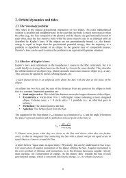
Hydromagnetic waves in Earth's core and their influence on ...

iAbstractIn this thesis east-west motions of Earth’s magnetic field on time scales of centuriesto millennia <strong>and</strong> associated patterns of field evolution at the <strong>core</strong> surface are studied.The hypothesis that hydromagnetic <strong>waves</strong> <strong>in</strong> Earth’s <strong>core</strong> contribute to such changes is<strong>in</strong>vestigated by compar<strong>in</strong>g analysis of historical <strong>and</strong> archeomagnetic observations withpredictions from analytical <strong>and</strong> numerical wave models.Geomagnetic field models are analysed <strong>in</strong> order to quantify the characteristics of radialmagnetic field (B r ) evolution at the <strong>core</strong> surface. In the historical model gufm1, spatially<strong>and</strong> temporally coherent (wave-like) patterns are identified <strong>in</strong> B r . Particularly strik<strong>in</strong>gis a low latitude signal with azimuthal wavenumber m=5 that travels westwards at∼17 km yr −1 . Study<strong>in</strong>g the archeomagnetic model CALS7K.1, episodes of both eastward<strong>and</strong> westward motion of wave-like patterns <strong>in</strong> B r are observed. Analysis of the evolutionof fields <strong>and</strong> underly<strong>in</strong>g flows from geodynamo simulations is used to illustrate that<strong>in</strong>ability to resolve the smallest length scales of the field makes quantitative <strong>in</strong>ferencesconcern<strong>in</strong>g the flow difficult, unless the flow is large scale. Furthermore, it is foundazimuthal motions of patterns <strong>in</strong> B r can be produced by hydromagnetic <strong>waves</strong> <strong>in</strong> thesimulations. The rema<strong>in</strong>der of the thesis addresses whether hydromagnetic <strong>waves</strong> <strong>in</strong> the<strong>core</strong> could be the orig<strong>in</strong> of azimuthal geomagnetic secular variation.Magneto-Rossby <strong>waves</strong> driven by convection (with a dynamical balance between magneticforces, latitude-dependent Coriolis forces, <strong>and</strong> buoyancy forces) are proposed as asuitable c<strong>and</strong>idate for hydromagnetic <strong>waves</strong> <strong>in</strong> the <strong>core</strong>. When driven by thermal convection,such <strong>waves</strong> propagate on the thermal diffusion time scale. Convection-drivenmagneto-Rossby <strong>waves</strong> are found to exhibit dispersive behaviour <strong>and</strong> a dependence ofpropagation speed on latitude. It is shown that such hydromagnetic <strong>waves</strong> <strong>in</strong> the <strong>core</strong>could produce wave-like patterns <strong>in</strong> B r <strong>in</strong> two ways. One mechanism <strong>in</strong>volves the distortionof toroidal magnetic field with<strong>in</strong> the <strong>core</strong> by wave flows produc<strong>in</strong>g new, spatiallyperiodic <strong>and</strong> azimuthally drift<strong>in</strong>g, concentrations of B r . This mechanism is <strong>in</strong>vestigatedus<strong>in</strong>g a 3D, l<strong>in</strong>ear, dynamical model with spherical geometry <strong>and</strong> an imposed toroidalmagnetic field. When this toroidal magnetic field is equatorially symmetric, wave-likepatterns <strong>in</strong> B r centred on the equator are obta<strong>in</strong>ed. Wave flows are found to consist ofalternat<strong>in</strong>g regions of flow convergence <strong>and</strong> divergence close to the outer boundary. Asecond mechanism whereby hydromagnetic <strong>waves</strong> can produce spatially <strong>and</strong> temporallycoherent patterns <strong>in</strong> B r <strong>in</strong>volves advection of exist<strong>in</strong>g B r by the wave flows. This mechanismis studied us<strong>in</strong>g a 1D, diffusionless, analytical model <strong>and</strong> a 2D numerical modelon a spherical surface <strong>in</strong>clud<strong>in</strong>g limited magnetic diffusion. It is found that propagat<strong>in</strong>gconcentrations <strong>in</strong> B r are produced that pulsate <strong>in</strong> amplitude if the wave propagationspeed is faster than the fluid motions with<strong>in</strong> the wave. Both mechanisms could feasiblybe <strong>in</strong>volved <strong>in</strong> produc<strong>in</strong>g the wave-like patterns <strong>in</strong> B r identified at the <strong>core</strong> surface.

iiiContents1 Introduction 11.1 Overview . . . . . . . . . . . . . . . . . . . . . . . . . . . . . . . . . . . . 11.2 Earth’s magnetic field . . . . . . . . . . . . . . . . . . . . . . . . . . . . . 11.2.1 Observations of the geomagnetic field . . . . . . . . . . . . . . . . 11.2.2 Geomagnetic secular variation . . . . . . . . . . . . . . . . . . . . . 31.3 Orig<strong>in</strong> of the geomagnetic field <strong>in</strong> Earth’s outer <strong>core</strong> . . . . . . . . . . . . 51.3.1 Internal source of the geomagnetic field . . . . . . . . . . . . . . . 51.3.2 Physical properties of the outer <strong>core</strong> . . . . . . . . . . . . . . . . . 71.3.3 Energy sources <strong>and</strong> <strong>core</strong> motions . . . . . . . . . . . . . . . . . . . 81.3.4 The geodynamo mechanism . . . . . . . . . . . . . . . . . . . . . . 81.3.5 Causes of geomagnetic secular variation, flow at the <strong>core</strong> surface<strong>and</strong> changes <strong>in</strong> the length of day . . . . . . . . . . . . . . . . . . . 101.4 <strong>Hydromagnetic</strong> <strong>waves</strong> <strong>in</strong> the <strong>core</strong> <strong>and</strong> geomagnetic secular variation . . . 121.4.1 An example of a hydromagnetic wave <strong>in</strong> the <strong>core</strong> <strong>and</strong> its possibleeffects . . . . . . . . . . . . . . . . . . . . . . . . . . . . . . . . . . 121.4.2 Previous studies l<strong>in</strong>k<strong>in</strong>g hydromagnetic <strong>waves</strong> <strong>and</strong> geomagneticsecular variation . . . . . . . . . . . . . . . . . . . . . . . . . . . . 131.5 Thesis aims <strong>and</strong> structure . . . . . . . . . . . . . . . . . . . . . . . . . . . 142 A space-time process<strong>in</strong>g <strong>and</strong> spectral analysis methodology 162.1 Overview . . . . . . . . . . . . . . . . . . . . . . . . . . . . . . . . . . . . 162.2 Visualisation <strong>and</strong> analysis techniques . . . . . . . . . . . . . . . . . . . . . 172.2.1 Grid<strong>in</strong>g models <strong>in</strong> space <strong>and</strong> time . . . . . . . . . . . . . . . . . . . 172.2.2 Construction <strong>and</strong> <strong>in</strong>terpretation of time-longitude (TL) plots . . . 172.2.3 Construction <strong>and</strong> <strong>in</strong>terpretation of frequency-wavenumber (FK)power spectra . . . . . . . . . . . . . . . . . . . . . . . . . . . . . . 202.2.4 Construction <strong>and</strong> <strong>in</strong>terpretation of latitude-azimuthal speed (LAS)power plots, us<strong>in</strong>g a Radon transform technique . . . . . . . . . . 232.3 Synthetic field models used for methodology test<strong>in</strong>g . . . . . . . . . . . . 272.4 Removal of the time-averaged axisymmetric field . . . . . . . . . . . . . . 302.5 High-pass filter<strong>in</strong>g . . . . . . . . . . . . . . . . . . . . . . . . . . . . . . . 342.5.1 Motivation for high-pass temporal filter<strong>in</strong>g of field models . . . . . 342.5.2 Filter specification <strong>and</strong> implementation . . . . . . . . . . . . . . . 34

iv2.5.3 Filter warm-up effects <strong>and</strong> choice of filter order. . . . . . . . . . . 352.5.4 Influence of filter type on processed field . . . . . . . . . . . . . . . 362.5.5 Criteria for choice of filter cut-off period t c . . . . . . . . . . . . . 372.5.6 Measur<strong>in</strong>g field variations captured as a function of t c . . . . . . . 372.5.7 Discussion of properties of form of processed field for a range offilter cut-off periods . . . . . . . . . . . . . . . . . . . . . . . . . . 392.6 Geographical distribution of azimuthal speeds of field features . . . . . . . 432.7 Temporal variations <strong>in</strong> latitude-azimuthal speed (LAS) power plots . . . . 442.8 Analysis of hemispherically conf<strong>in</strong>ed signals . . . . . . . . . . . . . . . . . 452.9 Frequency-wavenumber filter<strong>in</strong>g techniques . . . . . . . . . . . . . . . . . 492.10 Discussion . . . . . . . . . . . . . . . . . . . . . . . . . . . . . . . . . . . . 502.11 Summary . . . . . . . . . . . . . . . . . . . . . . . . . . . . . . . . . . . . 533 Application of the space-time spectral analysis technique to the historicalgeomagnetic field model gufm1 543.1 Introduction . . . . . . . . . . . . . . . . . . . . . . . . . . . . . . . . . . . 543.2 Description of field evolution processes <strong>in</strong> the azimuthal direction . . . . . 553.2.1 Unprocessed radial magnetic field (B r ) . . . . . . . . . . . . . . . . 553.2.2 Radial magnetic field without time-averaged axisymmetric part(B r − ¯B r ) . . . . . . . . . . . . . . . . . . . . . . . . . . . . . . . . 583.2.3 Radial magnetic field with time averaged axisymmetric componentremoved <strong>and</strong> high pass filtered (˜B r ) . . . . . . . . . . . . . . . . . 613.2.4 Comparison of ˜B r when filter<strong>in</strong>g threshold is 400 years <strong>and</strong> 600 years 653.2.5 Spherical harmonic power spectrum for ˜B r . . . . . . . . . . . . . 673.3 Isolation <strong>and</strong> description of field evolution modes <strong>in</strong> ˜B r . . . . . . . . . . 683.4 Geographical trends <strong>in</strong> azimuthal speeds of field features . . . . . . . . . . 703.5 Hemispherical differences <strong>in</strong> field evolution processes . . . . . . . . . . . . 713.6 Temporal variations <strong>in</strong> field evolution processes . . . . . . . . . . . . . . . 723.7 Determ<strong>in</strong>ation of dispersion by wavenumber filter<strong>in</strong>g ˜B r from gufm1 . . . 753.8 Summary . . . . . . . . . . . . . . . . . . . . . . . . . . . . . . . . . . . . 774 Application of the space-time spectral analysis technique to the archeomagneticfield model CALS7K.1 804.1 Introduction . . . . . . . . . . . . . . . . . . . . . . . . . . . . . . . . . . . 804.2 Comparison of CALS7K.1h to gufm1d . . . . . . . . . . . . . . . . . . . . 814.2.1 Creation of gufm1d <strong>and</strong> spherical harmonic power spectra . . . . . 814.2.2 Comparison of unprocessed radial magnetic field (B r ) . . . . . . . 814.2.3 High pass filter<strong>in</strong>g <strong>and</strong> the variability captured by gufm1d <strong>and</strong>CALS7K.1h . . . . . . . . . . . . . . . . . . . . . . . . . . . . . . . 844.3 Space-time analysis of CALS7K.1 . . . . . . . . . . . . . . . . . . . . . . . 88

v4.3.1 Analysis of unprocessed radial magnetic field (B r ) for full span ofCALS7K.1 . . . . . . . . . . . . . . . . . . . . . . . . . . . . . . . 884.3.2 Analysis of ˜B r from 2000 B.C. to 1700 A.D. . . . . . . . . . . . . . 914.3.3 Hemispherical differences <strong>in</strong> field evolution processes . . . . . . . . 954.3.4 Discussion . . . . . . . . . . . . . . . . . . . . . . . . . . . . . . . . 954.4 Summary of application of space-time spectral analysis to CALS7K.1 . . . 985 Application of the space-time spectral analysis technique to outputfrom a convection-driven geodynamo model 995.1 Introduction . . . . . . . . . . . . . . . . . . . . . . . . . . . . . . . . . . . 995.2 DYN1: (E=2×10 −2 , P r=1, P r m =10, Ra/Ra c ∼ 3, R m ∼ 100) . . . . . . 1005.2.1 Radial magnetic field (B r ) from DYN1 . . . . . . . . . . . . . . . . 1015.2.2 Velocity field from DYN1 . . . . . . . . . . . . . . . . . . . . . . . 1085.2.3 Discussion of results from DYN1 . . . . . . . . . . . . . . . . . . . 1155.3 DYN2: (E=3×10 −4 , P r=1, P r m =3, Ra/Ra c ∼ 32, R m ∼ 500) . . . . . . 1165.3.1 Undamped radial magnetic field (B r ) from DYN2 . . . . . . . . . 1175.3.2 Radial magnetic field from DYN2 (B r ) with l > 10 damped . . . . 1225.3.3 Velocity field from DYN2 . . . . . . . . . . . . . . . . . . . . . . . 1255.3.4 Discussion of results from DYN2 <strong>and</strong> DYN2d . . . . . . . . . . . . 1285.4 Summary . . . . . . . . . . . . . . . . . . . . . . . . . . . . . . . . . . . . 1326 Theory of hydromagnetic <strong>waves</strong> <strong>in</strong> rapidly rotat<strong>in</strong>g fluids 1346.1 Introduction . . . . . . . . . . . . . . . . . . . . . . . . . . . . . . . . . . . 1346.2 Survey of hydromagnetic wave literature . . . . . . . . . . . . . . . . . . . 1356.3 Lead<strong>in</strong>g order force balance associated with hydromagnetic <strong>waves</strong> <strong>in</strong> rapidlyrotat<strong>in</strong>g fluids . . . . . . . . . . . . . . . . . . . . . . . . . . . . . . . . . . 1366.4 <strong>Hydromagnetic</strong> <strong>waves</strong> driven by convection, <strong>in</strong> a rotat<strong>in</strong>g plane layer . . . 1396.4.1 Effect of diffusion on hydromagnetic <strong>waves</strong> . . . . . . . . . . . . . 1416.5 Influence of spherical geometry on hydromagnetic <strong>waves</strong> . . . . . . . . . . 1436.5.1 Variation of Coriolis force with latitude: Hide’s β-plane model . . 1436.5.2 Full spherical geometry: the special case of the Malkus field . . . . 1476.6 Instability mechanisms for hydromagnetic <strong>waves</strong> . . . . . . . . . . . . . . 1506.6.1 Magnetically-driven <strong>in</strong>stabilities <strong>in</strong> a rapidly rotat<strong>in</strong>g fluid . . . . . 1516.6.2 Convection-driven <strong>in</strong>stabilities <strong>in</strong> the presence of a magnetic field<strong>and</strong> rapid rotation . . . . . . . . . . . . . . . . . . . . . . . . . . . 1536.7 Nonl<strong>in</strong>ear <strong>in</strong>fluences on hydromagnetic <strong>waves</strong> . . . . . . . . . . . . . . . . 1656.8 Influence of stratification on hydromagnetic <strong>waves</strong> . . . . . . . . . . . . . 1686.9 Summary . . . . . . . . . . . . . . . . . . . . . . . . . . . . . . . . . . . . 1687 Convection-driven, l<strong>in</strong>ear hydromagnetic <strong>waves</strong> <strong>in</strong> a sphere 1707.1 Introduction . . . . . . . . . . . . . . . . . . . . . . . . . . . . . . . . . . . 1707.2 Manipulation of govern<strong>in</strong>g equations <strong>in</strong>to eigenvalue form . . . . . . . . . 171

vi7.2.1 Govern<strong>in</strong>g equations . . . . . . . . . . . . . . . . . . . . . . . . . . 1717.2.2 Toroidal-poloidal expansion <strong>and</strong> equations govern<strong>in</strong>g the evolutionof the scalar fields . . . . . . . . . . . . . . . . . . . . . . . . . . . 1727.2.3 Assumptions regard<strong>in</strong>g equatorial symmetry of <strong>waves</strong> . . . . . . . 1737.2.4 Expansion of scalars <strong>in</strong>to spherical harmonics <strong>and</strong> Chebyshev polynomials. . . . . . . . . . . . . . . . . . . . . . . . . . . . . . . . . 1737.2.5 Boundary conditions . . . . . . . . . . . . . . . . . . . . . . . . . . 1747.2.6 Formulation of the eigenvalue problem . . . . . . . . . . . . . . . . 1767.3 Numerical solution of eigenvalue problem . . . . . . . . . . . . . . . . . . 1777.3.1 Criteria for except<strong>in</strong>g <strong>and</strong> rejected eigenvalues . . . . . . . . . . . 1787.3.2 Benchmark<strong>in</strong>g the eigenvalue solver code . . . . . . . . . . . . . . 1787.4 Results . . . . . . . . . . . . . . . . . . . . . . . . . . . . . . . . . . . . . . 1797.4.1 Wave types <strong>and</strong> <strong>their</strong> structure . . . . . . . . . . . . . . . . . . . . 1807.4.2 Dependence on E . . . . . . . . . . . . . . . . . . . . . . . . . . . . 1877.4.3 Dependence on Λ . . . . . . . . . . . . . . . . . . . . . . . . . . . . 1887.4.4 Dependence on P r . . . . . . . . . . . . . . . . . . . . . . . . . . . 1907.4.5 Dependence on P r m . . . . . . . . . . . . . . . . . . . . . . . . . . 1917.5 Discussion of implications for <strong>waves</strong> <strong>in</strong> Earth’s <strong>core</strong> . . . . . . . . . . . . . 1927.6 Summary . . . . . . . . . . . . . . . . . . . . . . . . . . . . . . . . . . . . 1938 Patterns of magnetic field evolution caused by wave flows 1948.1 Introduction . . . . . . . . . . . . . . . . . . . . . . . . . . . . . . . . . . . 1948.2 1D model of a wave flow act<strong>in</strong>g on a magnetic field . . . . . . . . . . . . . 1958.2.1 Frozen-flux equation for field evolution . . . . . . . . . . . . . . . . 1958.2.2 Chang<strong>in</strong>g reference frame to move along with wave flow . . . . . . 1978.2.3 Solution us<strong>in</strong>g the method of characteristics . . . . . . . . . . . . . 1988.2.4 Discussion of solutions to 1D frozen flux wave flow problem . . . . 2028.2.5 Steady state balance between advection <strong>and</strong> diffusion . . . . . . . 2088.3 2D wave flow act<strong>in</strong>g on a radial magnetic field at a spherical surface . . . 2128.3.1 2D model equations <strong>and</strong> imposed flow . . . . . . . . . . . . . . . . 2128.3.2 Numerical solution of 2D wave flow model . . . . . . . . . . . . . . 2148.3.3 A parameter survey of results from the 2D wave flow model . . . . 2188.3.4 Spatial characteristics of field evolution <strong>in</strong> the 2D wave flow model 2228.3.5 Evolution of realistic magnetic fields produced by wave flows . . . 2308.3.6 Impact of crustal filter<strong>in</strong>g <strong>and</strong> sources of hemispherical asymmetry 2348.3.7 Discussion of implications for mechanisms of geomagnetic secularvariation <strong>and</strong> <strong>core</strong> flow <strong>in</strong>version techniques . . . . . . . . . . . . . 2378.3.8 Summary . . . . . . . . . . . . . . . . . . . . . . . . . . . . . . . . 2409 Conclusions <strong>and</strong> suggestions for further research 2419.1 A synthesis of results . . . . . . . . . . . . . . . . . . . . . . . . . . . . . . 2419.2 Summary of work carried out <strong>and</strong> ma<strong>in</strong> conclusions . . . . . . . . . . . . . 245

vii9.3 Suggestions of extensions <strong>and</strong> directions for future research . . . . . . . . 246A Historical geomagnetic field model gufm1 249A.1 Historical observations of Earth’s magnetic field . . . . . . . . . . . . . . . 249A.2 Field modell<strong>in</strong>g methodology . . . . . . . . . . . . . . . . . . . . . . . . . 249A.3 Comparison to observatory data . . . . . . . . . . . . . . . . . . . . . . . 254A.4 Limitations of gufm1 . . . . . . . . . . . . . . . . . . . . . . . . . . . . . . 257A.5 Grid<strong>in</strong>g of gufm1 for analysis on <strong>core</strong> surface . . . . . . . . . . . . . . . . 258B The archeomagnetic field model CALS7K.1 259B.1 Introduction . . . . . . . . . . . . . . . . . . . . . . . . . . . . . . . . . . . 259B.2 Data sources . . . . . . . . . . . . . . . . . . . . . . . . . . . . . . . . . . 259B.3 Spatial <strong>and</strong> temporal distribution of data . . . . . . . . . . . . . . . . . . 260B.4 Uncerta<strong>in</strong>ty estimates . . . . . . . . . . . . . . . . . . . . . . . . . . . . . 262B.5 Field modell<strong>in</strong>g methodology . . . . . . . . . . . . . . . . . . . . . . . . . 263B.6 Characteristics <strong>and</strong> evaluation of the model CALS7K.1 . . . . . . . . . . . 264B.7 Grid<strong>in</strong>g of CALS7K.1 for analysis on <strong>core</strong> surface . . . . . . . . . . . . . . 264C A 3D, convection-driven, spherical shell dynamo model (MAGIC) 265C.1 Introduction . . . . . . . . . . . . . . . . . . . . . . . . . . . . . . . . . . . 265C.2 Model equations <strong>and</strong> boundary conditions . . . . . . . . . . . . . . . . . . 265C.3 Numerical solution . . . . . . . . . . . . . . . . . . . . . . . . . . . . . . . 266C.4 Parameters of models studied . . . . . . . . . . . . . . . . . . . . . . . . . 267C.5 Relat<strong>in</strong>g geodynamo model output to the Earth: problems with time scales268D Equations govern<strong>in</strong>g hydromagnetic <strong>waves</strong> <strong>in</strong> Earth’s outer <strong>core</strong> 270D.1 Bouss<strong>in</strong>esq hydromagnetic equations for convection <strong>in</strong> a rotat<strong>in</strong>g fluid . . 270D.2 L<strong>in</strong>earised govern<strong>in</strong>g equations . . . . . . . . . . . . . . . . . . . . . . . . 271D.3 Non-dimensionalisation us<strong>in</strong>g the viscous time scale . . . . . . . . . . . . 272E Equatorial symmetry considerations <strong>in</strong> spherical geometry 274E.1 Overview . . . . . . . . . . . . . . . . . . . . . . . . . . . . . . . . . . . . 274E.2 Equatorial symmetry operations . . . . . . . . . . . . . . . . . . . . . . . 274E.3 Symmetry <strong>in</strong> l<strong>in</strong>ear models of thermally-driven hydromagnetic <strong>waves</strong> . . . 276E.4 Equatorial symmetry of B r at the <strong>core</strong> surface <strong>and</strong> its relation to equatorialsymmetry of flows at the <strong>core</strong> surface . . . . . . . . . . . . . . . . . . 277F Animations 278F.1 Animations as a visualisation tool . . . . . . . . . . . . . . . . . . . . . . 278F.2 Construction of animations . . . . . . . . . . . . . . . . . . . . . . . . . . 278F.3 Locations of animations . . . . . . . . . . . . . . . . . . . . . . . . . . . . 278References 283

viiiList of Figures1.1 The geomagnetic field at Earth’s surface <strong>in</strong> 2000 A.D. . . . . . . . . . . . 21.2 Westward drift of the geomagnetic field from 1600 to 1950 A.D. . . . . . . 41.3 Structure of Earth’s <strong>in</strong>terior <strong>in</strong>ferred from seismology . . . . . . . . . . . . 51.4 Radial magnetic field B r at the <strong>core</strong> surface <strong>in</strong> 2000 A.D. . . . . . . . . . 61.5 Flow at the <strong>core</strong> surface from 1840 to 1990 A.D. . . . . . . . . . . . . . . 111.6 A possible hydromagnetic wave <strong>in</strong> Earth’s <strong>core</strong> . . . . . . . . . . . . . . . 132.1 Relation of latitude-longitude maps to time-longitude (TL) plots . . . . . 182.2 Time-longitude (TL) plots from meteorology <strong>and</strong> oceanography . . . . . . 192.3 Example of frequency-wavenumber (FK) power spectra . . . . . . . . . . . 212.4 Radon transform of a time-longitude plot. . . . . . . . . . . . . . . . . . . 242.5 Construction of latitude-azimuthal speed (LAS) power plots . . . . . . . . 262.6 Analysis of H from SPOTNB <strong>and</strong> WAVENB field models . . . . . . . . . 282.7 Analysis of background field evolution model (BACK) . . . . . . . . . . . 292.8 Properties of field H from synthetic models SPOT <strong>and</strong> WAVE . . . . . . 312.9 Time-averaged, axisymmetric fields ¯H from SPOT <strong>and</strong> WAVE . . . . . . 322.10 SPOT <strong>and</strong> WAVE (H- ¯H) field models. . . . . . . . . . . . . . . . . . . . . 332.11 Amplitude response of filter |F H | 2 <strong>in</strong> the frequency doma<strong>in</strong>. . . . . . . . . 352.12 Trials with 2nd, 3rd <strong>and</strong> 4th order Butterworth filters. . . . . . . . . . . . 352.13 Trials with Butterworth, Chebyshev <strong>and</strong> Elliptic types of filters . . . . . . 362.14 Field variations captured as a function of filter cut-off period . . . . . . . 382.15 SPOT <strong>and</strong> WAVE ˜H, high pass filtered with t c = 200yrs. . . . . . . . . . 402.16 SPOT <strong>and</strong> WAVE ˜H, high pass filtered with t c = 400yrs. . . . . . . . . . 412.17 SPOT <strong>and</strong> WAVE ˜H, high pass filtered with t c = 600yrs. . . . . . . . . . 422.18 Geographical distribution <strong>and</strong> speeds of field features. . . . . . . . . . . . 442.19 Temporal changes <strong>in</strong> latitude-azimuthal speed power plots . . . . . . . . . 452.20 Analysis of a hemispherically conf<strong>in</strong>ed wave. . . . . . . . . . . . . . . . . . 472.21 Analysis of hemispherically conf<strong>in</strong>ed wave <strong>and</strong> background field. . . . . . . 482.22 FK-filtered, reconstructed SPOTNB <strong>and</strong> WAVENB field models. . . . . . 512.23 FK-filtered, reconstructed SPOT <strong>and</strong> WAVE field models. . . . . . . . . . 52

ix3.1 Snapshots of B r from gufm1 at the <strong>core</strong> surface . . . . . . . . . . . . . . . 563.2 TL plots <strong>and</strong> FK power spectra of B r from gufm1 . . . . . . . . . . . . . 573.3 Latitude-aziumuthal speed (LAS) power plot of B r from gufm1 . . . . . . 583.4 Snapshots of (B r − ¯B r ) from gufm1 at the <strong>core</strong> surface . . . . . . . . . . . 593.5 TL plots <strong>and</strong> FK power spectra of (B r − ¯B r ) from gufm1 . . . . . . . . . 603.6 Latitude-azimuthal speed power plot of (B r - ¯B r ) from gufm1 . . . . . . . . 613.7 B r variations captured by ˜B r . . . . . . . . . . . . . . . . . . . . . . . . . . 623.8 Snapshots of ˜B r from gufm1 at the <strong>core</strong> surface . . . . . . . . . . . . . . . 633.9 TL plots <strong>and</strong> FK power spectra of ˜B r . . . . . . . . . . . . . . . . . . . . 643.10 Latitude-azimuthal speed (LAS) power plot of ˜B r from gufm1 . . . . . . . 653.11 ˜B r from gufm1, for filter cut-offs of t c =400yrs <strong>and</strong> 600 yrs . . . . . . . . . 663.12 Spherical harmonic power spectra of B r , (B r - ¯B r ), <strong>and</strong> ˜B r from gufm1 . . 673.13 Snapshots <strong>and</strong> LAS plots of˜Brecr from gufm1; m= 7, 5 <strong>and</strong> 3 . . . . . . . 693.14 Geographical variations <strong>in</strong> azimuthal speeds of ˜B r from gufm1 . . . . . . 703.15 Hemispherical differences <strong>in</strong> field evolution <strong>in</strong> gufm1. . . . . . . . . . . . . 733.16 Temporal evolution of LAS plots of ˜B r from gufm1 . . . . . . . . . . . . . 743.17 LAS plots from gufm1 of (B r − ¯B r ) filtered by wavenumber . . . . . . . . 763.18 Wavenumber versus azimuthal speed of (B r − ¯B r ) at 0 ◦ N. . . . . . . . . . 784.1 Spectra from gufm1 compared to CALSK7.1h <strong>and</strong> gufm1d . . . . . . . . . 824.2 Comparison of snapshots of B r from CALS7K.1h <strong>and</strong> gufm1d . . . . . . . 834.3 TL plots of B r from CALS7K.1h <strong>and</strong> gufm1d . . . . . . . . . . . . . . . . 854.4 Variation <strong>in</strong> CALS7K.1h compared to gufm1d <strong>and</strong> gufm1. . . . . . . . . . 864.5 LAS power plots of ˜B r from CALS7K.1h <strong>and</strong> gufm1d . . . . . . . . . . . 874.6 Snapshots of B r from CALS7K.1 from 5000B.C. to 1750A.D. . . . . . . . 894.7 TL plots of B r from CALS7K.1. . . . . . . . . . . . . . . . . . . . . . . . 904.8 Variation <strong>in</strong> CALS7K.1 as a function of filter threshold period. . . . . . . 924.9 TL <strong>and</strong> FK plots of ˜B r from CALS7K.1 2000B.C to 1700A.D. . . . . . . . 934.10 LAS plots of ˜B r of CALS7K.1 from 2000B.C to 1700A.D. . . . . . . . . . 944.11 Hemispherical differences <strong>in</strong> field evolution <strong>in</strong> CALS7K.1. . . . . . . . . . 964.12 TL, FK <strong>and</strong> LAS plots from CALS7K.1 <strong>and</strong> gufm1. . . . . . . . . . . . . . 975.1 Snapshots of B r from DYN1 at r = r 0 . . . . . . . . . . . . . . . . . . . . 1025.2 TL plots <strong>and</strong> FK power spectra of B r from DYN1 . . . . . . . . . . . . . 1035.3 B r variation captured by ˜B r <strong>in</strong> DYN1 as function of filter cut-off. . . . . . 1045.4 LAS plots of ˜B r from DYN1 for a range of filter thresholds . . . . . . . . 105

x5.5 Snapshots of ˜B r from DYN1 at r = r 0 . . . . . . . . . . . . . . . . . . . . 1065.6 TL plots <strong>and</strong> FK power spectra of ˜B r from DYN1 . . . . . . . . . . . . . 1075.7 Snapshots of u r from DYN1 at 0.96r 0 . . . . . . . . . . . . . . . . . . . . 1095.8 TL plots, FK power spectra <strong>and</strong> LAS plot of u r from DYN1 . . . . . . . . 1105.9 Snapshots of u φ from DYN1 at 0.96r 0 . . . . . . . . . . . . . . . . . . . . 1135.10 TL plots, FK plot <strong>and</strong> LAS plot of u φ from DYN1 . . . . . . . . . . . . . 1145.11 Snapshots of B r from DYN2 at r = r 0 . . . . . . . . . . . . . . . . . . . . 1185.12 TL plots <strong>and</strong> FK power spectra of B r from DYN2 . . . . . . . . . . . . . 1195.13 B r variation captured by ˜B r <strong>in</strong> DYN2. . . . . . . . . . . . . . . . . . . . 1205.14 TL plots <strong>and</strong> FK power spectra of ˜B r from DYN2 . . . . . . . . . . . . . 1215.15 Snapshots of B r from DYN2d at r = r 0 . . . . . . . . . . . . . . . . . . . 1235.16 TL plots <strong>and</strong> FK power spectra of B r from DYN2d . . . . . . . . . . . . . 1245.17 B r variation captured by ˜B r <strong>in</strong> DYN2d chang<strong>in</strong>g filter cut-off. . . . . . . . 1255.18 TL plots <strong>and</strong> FK power spectra of ˜B r from DYN2d . . . . . . . . . . . . . 1265.19 Snapshots of U r from DYN2 at r = 0.975r 0 . . . . . . . . . . . . . . . . . 1275.20 TL plots <strong>and</strong> FK power spectra of u r from DYN2 . . . . . . . . . . . . . . 1295.21 Snapshots of u φ from DYN2 at r = 0.975r 0 . . . . . . . . . . . . . . . . . 1305.22 TL plots <strong>and</strong> FK power spectra of u φ from DYN2 . . . . . . . . . . . . . 1316.1 <strong>Hydromagnetic</strong> wave mechanisms <strong>in</strong> a rapidly rotat<strong>in</strong>g fluid . . . . . . . . 1386.2 Geometry of plane layer model of diffusionless MAC <strong>waves</strong>. . . . . . . . . 1396.3 The β-plane geometry employed by Hide (1966). . . . . . . . . . . . . . . 1446.4 Movement of fluid columns <strong>in</strong> th<strong>in</strong> <strong>and</strong> thick spherical shells. . . . . . . . 1466.5 Quasi-geostrophic (QG) annulus model geometry . . . . . . . . . . . . . . 1546.6 Stability diagram from Fearn (1979b) . . . . . . . . . . . . . . . . . . . . 1627.1 Benchmark<strong>in</strong>g of l<strong>in</strong>ear Magnetoconvection code . . . . . . . . . . . . . . 1797.2 Marg<strong>in</strong>al wave with m = 8, Λ=0.1, Λ=0.1, P r=1, P r m =1, E=10 −6 . . . 1817.3 Marg<strong>in</strong>al wave for Λ=1, m=5, P r = 10 −3 , P r m = 1, E = 10 −6 . . . . . . 1827.4 Marg<strong>in</strong>al wave with Λ=1, m=5, P r=0.1, P r m =10 −6 , E = 10 −6 . . . . . 1837.5 Marg<strong>in</strong>al wave with Λ=1, m=8, P r=1, P r m = 10 3 , E = 10 −6 . . . . . . . . 1847.6 Marg<strong>in</strong>al wave for m=3, Λ=10, P r=1, P r m =1, E=10 −6 . . . . . . . . . 1857.7 Dependence of Ra <strong>and</strong> ω on E for m=5, 8 . . . . . . . . . . . . . . . . . . 1877.8 Dependence of Ra <strong>and</strong> ω on Λ for m=2 to 9 . . . . . . . . . . . . . . . . . 1897.9 Dependence of Ra <strong>and</strong> ω on m for Λ=0.1 to 10 . . . . . . . . . . . . . . . 1907.10 Dependence of Ra <strong>and</strong> ω on P r for m=5, 8 . . . . . . . . . . . . . . . . . 1917.11 Dependence of Ra <strong>and</strong> ω on P r m for m=5, 8 . . . . . . . . . . . . . . . . 1928.1 Incompressible wave flow used <strong>in</strong> simple k<strong>in</strong>ematic model. . . . . . . . . . 196

xi8.2 Solution for evolution of B <strong>in</strong> the 1D problem, when |U| > |c ph |. . . . . . 2038.3 Solutions for B <strong>in</strong> the 1D problem, when |U| = |c ph |. . . . . . . . . . . . . 2058.4 Solutions for B <strong>in</strong> the 1D problem, when |U| < |c ph |. . . . . . . . . . . . . 2068.5 1D advection-diffusion balance: Field amplitude as a function of R clm. . . . 2118.6 2D wave flows on a spherical surface at an impenetrable boundary. . . . . 2138.7 Action of 2D wave flow on a axial dipole <strong>in</strong>itial magnetic field. . . . . . . 2198.8 Time series of evolution of maximum amplitude of B NADr . . . . . . . . . . 2218.9 Axial dipole evolution for flow with m=8, E S , c ph =0.05, U=5. . . . . . . 2238.10 Axial dipole evolution for flow with m=8, E A , c ph =0.05, U=5. . . . . . . 2248.11 Axial dipole evolution for flow with m=8, E S , c ph =5, U=5. . . . . . . . . 2258.12 Axial dipole evolution for flow with m=8, E A , c ph =5, U=5. . . . . . . . . 2268.13 Axial dipole evolution for flow with m=8, E S , c ph =50, U=5. . . . . . . . 2278.14 Axial dipole evolution for flow with m=8, E A , c ph =50, U=5. . . . . . . . 2288.15 Evolution of <strong>in</strong>itial B r with m = 1, 4. . . . . . . . . . . . . . . . . . . . . . 2308.16 B r from gufm1 at <strong>core</strong> surface <strong>in</strong> 1590 <strong>and</strong> 1790. . . . . . . . . . . . . . . 2318.17 Action of E S , m=8 flow on 1590 <strong>in</strong>itial field after 200yrs. . . . . . . . . . 2328.18 Action of E A , m=8 flow on 1590 <strong>in</strong>itial field after 200yrs. . . . . . . . . . 2338.19 B D r due to E S , m=8 flows act<strong>in</strong>g on 1590 B r for 150, 400 yrs. . . . . . . . 2369.1 B r perturbation caused by a m=5 hydromagnetic wave . . . . . . . . . . 2439.2 m=5 spatially coherent pattern <strong>in</strong>˜Brecr from gufm1 <strong>in</strong> 1830. . . . . . . . . 244A.1 Changes <strong>in</strong> spatial distribution of observations <strong>in</strong> gufm1. . . . . . . . . . . 250A.2 Temporal distribution of gufm1 observations. . . . . . . . . . . . . . . . . 251A.3 Comparison of gufm1 <strong>and</strong> observatory annual means (ma<strong>in</strong> field) . . . . . 255A.4 Comparison of gufm1 <strong>and</strong> observatory annual means (SV) . . . . . . . . . 256A.5 Spherical harmonic power spectra from gufm1. . . . . . . . . . . . . . . . 258B.1 Spatial locations <strong>and</strong> concentration of data <strong>in</strong> CALS7K.1 . . . . . . . . . 260B.2 Temporal distribution of decl<strong>in</strong>ation, <strong>in</strong>cl<strong>in</strong>ation <strong>in</strong> CALS7K.1 . . . . . . . 261

xiiList of Tables6.1 <strong>Hydromagnetic</strong> <strong>waves</strong> <strong>in</strong> a rotat<strong>in</strong>g, thermally convect<strong>in</strong>g fluid. . . . . . . 1697.1 Comparison of results from eigenvalue <strong>and</strong> time-stepp<strong>in</strong>g codes . . . . . . 180C.1 Parameters of dynamo models <strong>and</strong> estimates for Earth’s <strong>core</strong> . . . . . . . 268F.1 Animations from chapter 3 . . . . . . . . . . . . . . . . . . . . . . . . . . 279F.2 Animations from chapter 4 . . . . . . . . . . . . . . . . . . . . . . . . . . 279F.3 Animations from chapter 5 . . . . . . . . . . . . . . . . . . . . . . . . . . 280F.4 Animations from chapter 8 (Part i) . . . . . . . . . . . . . . . . . . . . . . 281F.5 Animations from chapter 8 (Part ii) . . . . . . . . . . . . . . . . . . . . . 282

xiiiNotation, physical constants, abbreviations<strong>and</strong> conventionsNotation for symbolsα Coefficient of volume expansionβ L<strong>in</strong>ear rate of change of Coriolis force <strong>in</strong> northward directionβ’ Magntitude of the background temperature gradientβ ∗ Upper boundary slope <strong>in</strong> QG model (see non-dimensional control parameters)γ Magnitude of gravitational accelerationSecular variation coefficients∆ Differential operator that is the angular part of r 2 ∇ 2∆T Temperature difference across spherical shell <strong>in</strong> dynamo model∆θ Grid spac<strong>in</strong>g <strong>in</strong> latitude∆φ Grid spac<strong>in</strong>g <strong>in</strong> longitude∆t Grid spac<strong>in</strong>g <strong>in</strong> timeδλ Difference between eigenvalues at two choices of trunctationɛ Heat per unit mass <strong>in</strong> the Bouss<strong>in</strong>esq thermal equationΘ Perturbation temperature field̂θ Unit vector <strong>in</strong> the meridional (north-south) directionθ Spherical polar co-latitude (angle south from North pole for Earth)η Magnetic diffusivity (1/µσ)κ Thermal diffusivity of the fluidΛ Elsasser number (see non-dimensional control parameters)Λ c Critical Elasser number for the onset of magnetic <strong>in</strong>stabilityλ Complex eigenvalue <strong>in</strong> magnetoconvection problemλ lat Latitudeλ ∗ latFixed latitude studied <strong>in</strong> β-plane modelλ <strong>in</strong> Eigenvalue of the <strong>in</strong>ertial wave problemλ S Spatial damp<strong>in</strong>g factor used to regularise field modelλ T Temporal damp<strong>in</strong>g factor used to regularise field modelµ Magnetic permeabilityµ 0 Magnetic permeability of non-permanently magnetised materialν K<strong>in</strong>ematic viscosity of the fluid∇ Gradient operator∇ H Horizontal component of the gradient operatorρ Fluid densityρ 0 Constant density of <strong>in</strong>compressible fluid, used <strong>in</strong> Bouss<strong>in</strong>esq approx.Φ Objective function m<strong>in</strong>imised dur<strong>in</strong>g <strong>in</strong>version for field modelγ mc/sl

xiv̂φ Unit vector <strong>in</strong> the eastward direction <strong>in</strong> spherical geometryAlso denotes eastward component when appears as a subscriptφ Spherical polar longitude (angle east from Greenwich meridion for Earth)φ’ Longitude co-ord<strong>in</strong>ate <strong>in</strong> reference frame drift<strong>in</strong>g along with 2D wave flowΨ Streamfunction of k<strong>in</strong>ematically prescribed, simple wave flowψ Spatial co-ord<strong>in</strong>ate <strong>in</strong> frame drift<strong>in</strong>g along with 1D wave flowσ Electrical conductivityτ η Magnetic diffusion time (D 2 /η)τ ν Viscous diffusion time (D 2 /ν)Ω Angular rotation rate of system̂Ω Unit vector <strong>in</strong> the direction of the angular rotation rate vectorΩ Magnitude of the angular rotation rate of systemω Angular frequency of wave or signalω M Angular frequency of simple hydromagnetic (Alfven) waveω A Angular frequency of <strong>in</strong>ternal gravity waveω C Angular frequency of <strong>in</strong>ertial waveω MC Angular frequency of slow Magnetic-Coriolis (MC) waveω c Angular frequency of wave at the onset of <strong>in</strong>stabilityχ Streamfunction of flow <strong>in</strong> Quasi-Geostrophic annulus modelAlso the normalised misfit of data to field modelΥ Accumlated drift rate of reference frame drift<strong>in</strong>g along with wave flowζ Component of fluid vorticity along the rotation axis <strong>in</strong> QG modelA Matrix of terms without time dependence <strong>in</strong> magnetoconvection problemA ijk Array l<strong>in</strong>k<strong>in</strong>g components of secular variation, magnetic field <strong>and</strong> flowB Matrix of terms with time dependence <strong>in</strong> magnetoconvection problemB Vector magnetic field (strictly referred to as magnetic flux density)B 0 Background magnetic field l<strong>in</strong>earised around̂B 0 Unit vector <strong>in</strong> the direction of the background magnetic fieldB 0 Magnitude of background (imposed) magnetic fieldB 0x Component of background magnetic field <strong>in</strong> the cartesian x directionB 0y Component of background magnetic field <strong>in</strong> the cartesian y directionB 0z Component of background magnetic field <strong>in</strong> the cartesian z directionB r Magntitude of magnetic field <strong>in</strong> the radial direction¯B r Time-averaged, axisymmetric, part of radial magnetic field˜B r (B r - ¯B r ), high pass filtered with cut-off period t c˜B rrec Reconstruction of particular modes of B r after mask-FK filter<strong>in</strong>g ˜B rB r0 Background radial magnetic fieldB r ’ Perturbation radial magnetic fieldBrNAD Non-axial dipole part of radial magnetic fieldB θ Amplitude of magnetic field <strong>in</strong> the southward directionB φ Amplitude of magnetic field <strong>in</strong> the eastward directionB Typical order of magnitude of magnetic field, used <strong>in</strong> scal<strong>in</strong>g argumentsb ′ Perturbation magnetic fieldb Perturbation magnetic field after dropp<strong>in</strong>g of ’

xvb Tb Pb xb yb zb mc/slb mc/s′lC eC mToroidal component of magnetic field perturbationPoloidal component of magnetic field perturbationPerturbation magnetic field component <strong>in</strong> the cartesian x directionPerturbation magnetic field component <strong>in</strong> the cartesian y directionPerturbation magnetic field component <strong>in</strong> the cartesian z directionSpherical harmonic coefficients for magnetic fieldSpherical harmonic coefficients for magnetic field <strong>in</strong> drift<strong>in</strong>g frameCovariance matrix for observations of the geomagnetic fieldCovariance matrix for geomagnetic field modelC Correction factor applied to Radon transform to remove directional biasC p Specific heat capacity at constant pressurec az Azimuthal speed of field featuresc ph Phase speed of wavec Radius of outer spherical shell <strong>in</strong> models, r cmb for EarthD Decl<strong>in</strong>ation: angle between the magnetic field <strong>and</strong> the northward directionAlso the spherical shell thickness for dynamo modelsAlso gap between cyl<strong>in</strong>ders for Quasi-Geostrophic annulus modelD L<strong>in</strong>ear operator aris<strong>in</strong>g under double curl of momentum <strong>and</strong> <strong>in</strong>duction eqnsd Vector of observations (data)d 0 Length scale of system under studyE Ekman number (see non-dimensional control parameters)E S Equatorially symmetricE A Equatorially anti-symmetrice Toroidal scalar for the velocity fieldF Magnitude of magnetic field vector, known as total <strong>in</strong>tensityF w Function determ<strong>in</strong><strong>in</strong>g time-dependent field morphology produced by wave flowF C Coriolis forceF H Frequency doma<strong>in</strong> representation of high pass filter used on H − ¯H to obta<strong>in</strong> ˜HF I Inertial forceF L Lorentz forceF Ohmic heat<strong>in</strong>g norm m<strong>in</strong>imised dur<strong>in</strong>g construction of field modelf Functional relat<strong>in</strong>g data to model <strong>in</strong> <strong>in</strong>version of field modelf Frequency (Fourier transform partner with time t)Also poloidal scalar for the velocity field <strong>in</strong> spherical geometryf c Coriolis parameter (2 Ω s<strong>in</strong> λ lat ) <strong>in</strong> plane modelsf c0 Constant Coriolis parameter <strong>in</strong> β-plane model (2 Ω s<strong>in</strong> λ ∗ lat )G v Summed absolute deviation of H from Ĥg Vector gravitational accelerationĝ Unit vector <strong>in</strong> the direction of the gravitational accelerationg toroidal scalar for the perturbation magnetic fieldglm Cos<strong>in</strong>e Gauss coefficientsH Generic time-dependent scalar field on a spherical surfaceH Fourier transform of generic scalar field HH R Radon transform of generic scalar field H¯H Time-averaged, axisymmetric part of H˜H H with time-averaged axisymmetric part removed <strong>and</strong> high pass filtered

xviĤ Time-averaged Ĥ˜H Time-averaged ˜HH rec Reconstruction of H after mask filter<strong>in</strong>g <strong>in</strong> the FK doma<strong>in</strong>H slope Difference <strong>in</strong> height btw <strong>in</strong>ner <strong>and</strong> outer cyl<strong>in</strong>ders <strong>in</strong> QG modelh Poloidal scalar for the perturbation magnetic fieldh m lS<strong>in</strong>e Gauss coefficientsI Incl<strong>in</strong>ation: angle between the magnetic field <strong>and</strong> the horizontal planeI 0 Zeroth-order spherical Bessel function√i −1, used with imag<strong>in</strong>ary numbersJ Electrical current densityJ H Internal heat<strong>in</strong>g rate per unit volumej Axial component of the perturbation electrical currentk Wavevector <strong>in</strong> direction of wave propagationk x Component of wavevector <strong>in</strong> the cartesian x directionk y Component of wavevector <strong>in</strong> the cartesian y directionk z Component of wavevector <strong>in</strong> the cartesian z directionk Wavenumber (Fourier transform partner with x)Also wavenumber of disturbance ( 2πL λ)L Number of spherical harmonic degrees used <strong>in</strong> representation of variablesL MC Typical length scale of MC wave disturbance <strong>in</strong> the field <strong>and</strong> flowL SV Maximium spherical harmonic degree of secular variationL U Maximium spherical harmonic degree used <strong>in</strong> expansiosn of flow scalarsL λ Wavelength of a general disturbanceL 1 L<strong>in</strong>ear operator premultiply<strong>in</strong>g (ẑ × u) <strong>in</strong> Malkus model of hydromagnetic <strong>waves</strong>L 2 L<strong>in</strong>ear operator premultiply<strong>in</strong>g u <strong>in</strong> Malkus model of hydromagnetic <strong>waves</strong>L 2 Angular momentum operator (angular part of Laplacian)l Spherical harmonic degreeM n Fourth order B-spl<strong>in</strong>e basis functionsm Field model obta<strong>in</strong>ed by <strong>in</strong>vert<strong>in</strong>g observationsm Azimuthal wavenumber (Fourier transform partner with φ)Also <strong>in</strong>dex for discrete po<strong>in</strong>ts on z axis <strong>in</strong> Radon transformAlso order of associated Legendre function Plmm c Azimuthal wavenumber of wave at the onset of <strong>in</strong>stabilityN Number of Chebyshev modes used <strong>in</strong> representation of variablesN t Number of discete time sample po<strong>in</strong>ts <strong>in</strong> a time series under studyN φ Number of discete spatial sample po<strong>in</strong>ts <strong>in</strong> a region under studyn In context of Radon transform, is an <strong>in</strong>dex for discrete angles of qO Order of magnitudeP Comb<strong>in</strong>ed mechanical <strong>and</strong> centrifugal pressuresP 0 Background pressureP ′ Perturbation pressure fieldP v Percentage ratio of R v to G v , each summed over all locationsP r Pr<strong>and</strong>tl number (see non-dimensional control parameters)P r m Magnetic Pr<strong>and</strong>tl number (see non-dimensional control parameters)Plm Associated Legendre function of degree l <strong>and</strong> order mQ Operator aris<strong>in</strong>g from double curl of momentum <strong>and</strong> <strong>in</strong>duction eqns

xviiq Angle used <strong>in</strong> def<strong>in</strong>ition of Radon transform (see figure 2.4)Also used to represent discrete time-steps <strong>in</strong> time-stepp<strong>in</strong>g algorithmR v Summed absolute deviations of ˜H from ̂˜HRa Rayleigh number (see non-dimensional control parameters)Ra c Critical Rayleigh number mark<strong>in</strong>g the onset of convectionRa m Modified Rayleigh number (see non-dimensional control parameters)R m Magnetic Reynolds number (see non-dimensional control parameters)Rm cl Magnetic Reynolds number used by Clark (1965)̂r Unit vector <strong>in</strong> the radial direction <strong>in</strong> spherical geometryr Displacement <strong>in</strong> the radial directionAlso denotes radial component when appears as a subscriptr cmb Core-mantle boundary radiusr i Inner radius of spherical shell under studyr 0 Outer radius of spherical shell under studyS Covariance matrix for spatial norm used <strong>in</strong> <strong>in</strong>version for field modelS Distribution of square of Radon transform amplitudes summed along zs Cyl<strong>in</strong>drical radiusAlso used <strong>in</strong> method of characteristics to def<strong>in</strong>e position on characteristicAlso surface poloidal scalar for flow on a spherical surfaceSL Array conta<strong>in</strong><strong>in</strong>g S (see previous entry) for all latitudesT Covariance matrix for temporal norm used <strong>in</strong> <strong>in</strong>version for field modelT Temperature fieldAlso flow toroidal scalar, for flow on a spherical surfaceT 0 Background temperature field l<strong>in</strong>earised around∇T 0 Vector background temperature gradient̂∇T 0 Unit vector along the background temperature gradientT H Time doma<strong>in</strong> representation of high pass filter used on H − ¯H to obta<strong>in</strong> ˜HT MC Typical time scale of MC wave disturbance <strong>in</strong> the field <strong>and</strong> flowT k Chebyschev polynomial of degree kt Timet c Threshold period for high-pass filter; signals slower than this are removedU 0 Background velocity fieldU Maximum amplitude of flow with<strong>in</strong> prescribed wave flowU rms Root mean square flow speedU zhang Form of <strong>in</strong>ertial wave flows on spherical boundary from Zhang et al. (2000)U Typical order of fluid flow (velocity), used <strong>in</strong> scal<strong>in</strong>g argumentsu Vector flow field (velocity field)Also perturbation to flow field after re-labell<strong>in</strong>gu ′ Flow perturbationAlso flow <strong>in</strong> reference frame mov<strong>in</strong>g with the flowu T Toroidal component of flowu P Poloidal component of flowu r Flow magntiude <strong>in</strong> the radial directionu θ Flow magntiude <strong>in</strong> the meridional (southward) directionu φ Flow magntiude <strong>in</strong> the zonal/azimuthal (eastward) directionFlow magntitude <strong>in</strong> cartesian x directionu x

xviiiu yu zVv nXx̂xxYŷyZẑzFlow magntitude <strong>in</strong> cartesian y directionFlow magntitude <strong>in</strong> cartesian z directionMagnetic potentialArray of azimuthal speeds derived us<strong>in</strong>g the Radon transform methodAmplitude of magnetic field <strong>in</strong> the northwards directionVector of unknown expansion coefficients <strong>in</strong> magnetoconvection problemUnit vector <strong>in</strong> the direction of the cartesian x-axisSpatial displacement (distance) along cartesian x-axisAlso displacement <strong>in</strong> the eastward direction <strong>in</strong> β-plane modelsAmplitude of magnetic field <strong>in</strong> the eastwards directionAlso represents spherical harmonic functionsUnit vector <strong>in</strong> the direction of the cartesian y-axisSpatial displacement (distance) along cartesian y-axisAmplitude of magnetic field <strong>in</strong> the radially <strong>in</strong>wards directionUnit vector <strong>in</strong> the direction of the cartesian z-axisSpatial displacement along the cartesian y-axisAlso x axis rotated by angle q when referr<strong>in</strong>g to the Radon transformNon-dimensional control parametersE =ν2Ωd 2 0Ekman numberP r = ν κPr<strong>and</strong>tl NumberP r m = ν ηMagnetic Pr<strong>and</strong>tl numberRa = |g| α |∇T 0| d 4 0κνRayleigh numberRa m = ERaP rModified Rayleigh numberR m = Urmsd 0ηMagnetic Reynolds numberR m = U kηMagnetic Reynolds number of Clark (1965)Λ = B2 02Ωµρ 0 ηβ ∗ = tan H slopeDElsasser numberAngle of slop<strong>in</strong>g upper boundary <strong>in</strong> QG modelValues adopted for physical constants, relevant to Earth’s <strong>core</strong>α=1.3 × 10 −5 K −1η=1.6 m 2 s −1κ=8.6×10 −6 m 2 s −1ν=10 −6 m 2 s −1ρ 0 =1×10 4 kg m −3µ 0 =4π × 10 −7 H m −1Ω=7.29 × 10 −5 s −1B 0 ∼ 1× 10 −3 Td 0 = r cmb − r i =3485 km - 1215 km=2260 kmγ=9.8 s −2|∇T 0 | ∼ 0.1 K km −1 (superadiabatic)(values taken from Gubb<strong>in</strong>s (2000))

xixAbbreviations <strong>and</strong> model namesA.D.BACKB.C.CALS7K.1CHAMPFKgufm1HEMIHEMINBIGRFLASMACMCSAC-CSPOTSPOTNBTLWAVEWAVENBAnno Dom<strong>in</strong>i (denotes year after 0 <strong>in</strong> the Christian calender)Synthetic field evolution model derived from spectrally smooth<strong>in</strong>g gufm1Before Christ (denotes years prior to 0 <strong>in</strong> the Christian calender)Geomagnetic field model of Korte <strong>and</strong> Constable (2005): 5000B.C.—1950A.D.CHAlleng<strong>in</strong>g M<strong>in</strong>isatellite Payload (German Earth-observ<strong>in</strong>g satellite)Frequency-wavenumber; refers to frequency-wavenumber power spectraGeomagnetic field model of Jackson et al. (2000): 1590—1990A.D.HEMINB with realistic background field BACK addedHemispherically conf<strong>in</strong>ed wave-like synthetic field evolution modelInternational Geomagnetic reference FieldLatitude-azimuthal speed; refers to latitude-azimuthal speed power plotsMagnetic-Archimedes-Coriolis, Archimedes means buoyancyMagnetic-CoriolisScientific Applications Satellite - C (Argent<strong>in</strong>e)Synthetic field model of drift<strong>in</strong>g spot plus background fieldSynthetic field model of drift<strong>in</strong>g spot without a background fieldTime-longitude; refers to time-longitude plotsSynthetic field model of a wave plus background fieldSynthetic field model of a wave without a background fieldConventionsS.I. units are employed throughout this thesisBlue-Orange colour scale is used to represent radial magnetic fieldsBlue-White-Red colour scale is used to represent temperature fieldsBlue-Green-Red colour scale is used to represent radial <strong>and</strong> azimuthal flows

xxAcknowledgementsI would like first to express my gratitude to Andrew Jackson for supervis<strong>in</strong>g my researchover the past four years. This thesis owes much to his suggestions for fruitful researchideas. Dur<strong>in</strong>g our many discussions I have benefited immensely from his deep knowledgeof geomagnetism <strong>and</strong> received sound advice on a wide range of practical matters. Hiswill<strong>in</strong>gness <strong>in</strong> allow<strong>in</strong>g me to pursue my own ideas <strong>and</strong> to provide constructive criticismhave been particularly appreciated.The geomagnetism group <strong>in</strong> Leeds has provided an extremely stimulat<strong>in</strong>g work environmentdur<strong>in</strong>g my time as a PhD student. I have learnt a great deal <strong>in</strong> discussionswith David Gubb<strong>in</strong>s who has always been generous with his time <strong>and</strong> been a constantsource of challeng<strong>in</strong>g <strong>and</strong> provocative ideas. Philip Livermore’s help <strong>and</strong> advice on howto survive as a research student were <strong>in</strong>valuable <strong>in</strong> my first few years. Ashley Willis hasprovided useful advice on numerics <strong>and</strong> dynamo related matters. Discussions with NickTeanby <strong>and</strong> Nicola Pressl<strong>in</strong>g have improved my underst<strong>and</strong><strong>in</strong>g of palaeomagnetism, <strong>and</strong>conversations with James While have helped illum<strong>in</strong>ate the subtleties of spectral analysis.Dur<strong>in</strong>g the f<strong>in</strong>al six months of this thesis the advice <strong>and</strong> encouragement of MathieuDumberry <strong>and</strong> Nicolas Gillet have been a great help. Their efforts <strong>in</strong> proof read<strong>in</strong>g areparticularly appreciated. I am also <strong>in</strong>debted to Stuart Borthwick <strong>and</strong> Nick Barber forrunn<strong>in</strong>g the geophysics computer system <strong>and</strong> to the secretarial staff for adm<strong>in</strong>istrativesupport.I have benefited greatly from the generosity of those who provided me with data, models<strong>and</strong> code. Andrew Jackson provided the historical geomagnetic field model gufm1that was used <strong>in</strong> chapter 3 <strong>and</strong> the <strong>core</strong> flow codes that were modified <strong>in</strong> chapter 8.Monika Korte provided the archeomagnetic field model CALS7K.1 that was analysed <strong>in</strong>chapter 4. Johannes Wicht provided output from the geodynamo model MAGIC thatwas analysed <strong>in</strong> chapter 5. Christopher Jones <strong>and</strong> Steven Worl<strong>and</strong> provided the basisof the l<strong>in</strong>ear magnetoconvection code that was used <strong>in</strong> chapter 7. I would also like toacknowledge the <strong>in</strong>sight of Stanislav Brag<strong>in</strong>sky <strong>and</strong> Raymond Hide who first suggestedthat <strong>waves</strong> <strong>in</strong> Earth’s <strong>core</strong> might contribute to geomagnetic secular variation.I am <strong>in</strong>debted to Emmanuel Dormy for host<strong>in</strong>g me dur<strong>in</strong>g a three month stay <strong>in</strong> Parisdur<strong>in</strong>g which my underst<strong>and</strong><strong>in</strong>g of hydromagnetic <strong>in</strong>stabilities greatly improved. Thewarm welcome given by V<strong>in</strong>cent Mor<strong>in</strong>, Aude Chambodut <strong>and</strong> Arnaud Chulliat as wellas the friendship of Ingo Ward<strong>in</strong>ski dur<strong>in</strong>g this time was much appreciated.F<strong>in</strong>ancially I must acknowledge the NERC for the studentship that supported me for thefirst three years of my study <strong>and</strong> the EU for the Marie-Curie fellowship which fundedmy time <strong>in</strong> Paris.I should also like to thank all my friends <strong>in</strong> the Earth Sciences department who havemade the past four years so enjoyable. In particular I would like to mention Kristof,L<strong>in</strong>dsey, Trudi, David Green, James Wookey, James Hammond, Andy C., Dan, Bryony,Andy G., Lucy, Siska, Steve, Laura, Carlos, Simon, Tung, as well as Murray, Andy B.,Dave B., Cathal, Nathan, James Cleverley <strong>and</strong> all the other regulars at the Eldon. Iam especially grateful to Ian Bastow, who has shared both an office <strong>and</strong> the stra<strong>in</strong>s ofwrit<strong>in</strong>g up with me dur<strong>in</strong>g the past year <strong>and</strong> somehow always managed to keep smil<strong>in</strong>g.Special thanks are due to my parents for <strong>their</strong> cont<strong>in</strong>u<strong>in</strong>g support, <strong>and</strong> to Edith for herunfail<strong>in</strong>g love <strong>and</strong> positivity.

1Chapter 1Introduction1.1 OverviewEarth possesses a global magnetic field that shields the planet from the effects of thesolar w<strong>in</strong>d (Jacobs, 1974; Kivelson <strong>and</strong> Russell, 1995; Langel <strong>and</strong> H<strong>in</strong>ze, 1998). Thisgeomagnetic field is not static, but fluctuates on a wide range of time scales from secondsto millions of years (Bloxham, 1995). Changes occurr<strong>in</strong>g over decades to millennia areknown as geomagnetic secular variation <strong>and</strong> have <strong>their</strong> orig<strong>in</strong> <strong>in</strong> motions of liquid metal<strong>in</strong> Earth’s <strong>core</strong>. This thesis focuses on the mechanism beh<strong>in</strong>d east-west motions of thegeomagnetic field <strong>and</strong> on the hypothesis that this <strong>in</strong>volves hydromagnetic wave motions<strong>in</strong> the <strong>core</strong>.In this <strong>in</strong>troductory chapter the background to the thesis is given. The observed natureof Earth’s magnetic field <strong>and</strong> its orig<strong>in</strong> <strong>in</strong> the outer <strong>core</strong> are described. Possible <strong>core</strong>dynamics govern<strong>in</strong>g magnetic field evolution are discussed, with particular attentiongiven to the wave hypothesis of geomagnetic secular variation. F<strong>in</strong>ally the aims of thethesis are set out <strong>and</strong> an outl<strong>in</strong>e of its structure is given.1.2 Earth’s magnetic field1.2.1 Observations of the geomagnetic fieldThe presence <strong>and</strong> structure of a magnetic field can be deduced by measur<strong>in</strong>g the force itexerts on mov<strong>in</strong>g charged particles <strong>and</strong> how this varies with location. The geomagneticfield is today measured by high precision vector <strong>and</strong> scalar magnetometers (see, forexamples, Forbes (1987)) <strong>in</strong> a worldwide network of geomagnetic observatories as well asby the Earth observ<strong>in</strong>g satellites Ørsted, CHAMP <strong>and</strong> SAC-C. The vector geomagneticfield B can be described by its strength <strong>in</strong> particular directions (northwards (X = −B θ ),eastwards (Y = B φ ) <strong>and</strong> radially <strong>in</strong>wards (Z = −B r )), or by the angle between itsorientation <strong>in</strong> the horizontal plane <strong>and</strong> the northward direction (decl<strong>in</strong>ation D), the

2 Chapter 1 — Introductionangle between its orientation <strong>and</strong> the horizontal plane at Earth’s surface (<strong>in</strong>cl<strong>in</strong>ation I),<strong>and</strong> the total <strong>in</strong>tensity of the field (F = |B| = (X 2 +Y 2 +Z 2 ) 1/2 ). Measurements of thesecomponents made at different locations are collected <strong>and</strong> used to produce geomagneticfield models (see, for example, Langel (1987)). An example of the D <strong>and</strong> F componentsof the IGRF (International Geomagnetic Reference field) at Earth’s surface for the year1122 M. MANDEA AND S. MACMILLAN: INTERNATIONAL GEOMAGNETIC REFERENCE FIELD: THE EIGHTH GENERATION2000 A.D. (M<strong>and</strong>ea <strong>and</strong> Macmillan, 2000) is presented <strong>in</strong> figure 1.1.(a) Decl<strong>in</strong>ation D(b) Total <strong>in</strong>tensity F1124 M. MANDEA AND S. MACMILLAN: INTERNATIONAL GEOMAGNETIC REFERENCE FIELD: THE EIGHFig. 1. Contour maps of the IGRF 2000 for D component (W<strong>in</strong>kel’s Tripel projection). Fig. 7. Contour maps of the IGRF 2000 for F component (W<strong>in</strong>kel’s Tripel projection).Figure 1.1: The geomagnetic field at Earth’s surface <strong>in</strong> 2000 A.D.The decl<strong>in</strong>ation D <strong>in</strong> (a) <strong>and</strong> the total <strong>in</strong>tensity F <strong>in</strong> (b) of the geomagnetic field atEarth’s surface <strong>in</strong> 2000 A.D. from the eighth generation IGRF (M<strong>and</strong>ea <strong>and</strong> Macmillan,2000). Contours of D are <strong>in</strong> degrees with dashed l<strong>in</strong>es <strong>in</strong>dicat<strong>in</strong>g negative values (magneticnorth to the east of true north means positive D) while <strong>in</strong> (b) the contours of Fare <strong>in</strong> nano-Tesla (nT). Plots are <strong>in</strong> W<strong>in</strong>kel’s Tripel projection.Acknowledgments. We would like to thank the Ørsted team, thestaff of magnetic observatories <strong>and</strong> survey organisations worldwidefor provid<strong>in</strong>g data on which the IGRF depends <strong>and</strong> the World DataCentres for data services. We also thank Stuart Mal<strong>in</strong> <strong>and</strong> VolodyaPapitashvili for comments, <strong>and</strong> the associate editor Frank Lowesfor useful discussions. All maps have been plotted us<strong>in</strong>g the GMTsoftware (Wessel <strong>and</strong> Smith, 1991). This paper is published withthe permission of the Director, British Geological Survey (NaturalEnvironment Research Council). This is IPGP contribution 1703.The positions of convergence of contours of D <strong>in</strong> figure 1.1a are the magnetic northReferencesBarton, C. E., International Geomagnetic Reference Field: the seventh generation,J. Geomag. Geoelectr., 49, 123–148, 1997.Chapman, S. <strong>and</strong> J. Bartels, Geomagnetism, 2 vols., pp. 1049, Oxford UniversityPress, London, 1940.Golovkov, V. P., T. N. Bondar, <strong>and</strong> I. A. Burdelnaya, Spatial-temporal model<strong>in</strong>gof the geomagnetic field for 1980–2000 period <strong>and</strong> a c<strong>and</strong>idateIGRF secular-variation model for 2000–2005, Earth Planets Space, 52,this issue, 1125–1135, 2000.Fig. 2. Contour maps of the IGRF 2000 for H component (W<strong>in</strong>kel’s Tripel projection).InternationalNoteAstronomicalthat the apparentUnion,s<strong>in</strong>gularityProc. 12th<strong>in</strong>Generalthe northernAssembly,polar regionHamburg,isan artifact of the plott<strong>in</strong>g rout<strong>in</strong>e.12B, 594–595, 1966.Langel, R. A., Ma<strong>in</strong> field, <strong>in</strong> Geomagnetism, edited by J. A. Jacobs, pp. 249–512, vol. I, Academic Press, London, 1987.Langlais, B. <strong>and</strong> M. M<strong>and</strong>ea, An IGRF c<strong>and</strong>idate ma<strong>in</strong> geomagnetic fieldmodel for epoch 2000 <strong>and</strong> a secular variation model for 2000–2005, Earth<strong>and</strong> south poles <strong>in</strong>dicated by navigational compasses. The high amplitude of F at highlatitudes <strong>and</strong> its low amplitude at low latitudes <strong>in</strong> figure 1.1b shows the predom<strong>in</strong>antlydipolar structure of the field at Earth surface. A consequence of the low F observed atSouth America is that solar radiation affects satellites most severely above this position.Underst<strong>and</strong><strong>in</strong>g the structure of the geomagnetic field <strong>and</strong> its changes is therefore importantnot just from the st<strong>and</strong>po<strong>in</strong>t of scientific curiosity, but also to telecommunication<strong>and</strong> other <strong>in</strong>dustries reliant on the operation of near-Earth satellites.In the past 1000 years humans have made direct measurements of the geomagneticfield us<strong>in</strong>g a variety of techniques. The first known observations of the direction of thegeomagnetic field were made by the Ch<strong>in</strong>ese scholar Shen Kua <strong>in</strong> 1088 A.D. (Needham,1962) but only isolated observations were made before the 16th century when use ofcompasses for long maritime voyages became widespread. Carl-Fredrich Gauss (1777A.D.— 1855 A.D.) devised a method for measur<strong>in</strong>g the <strong>in</strong>tensity of the geomagneticfield, stimulat<strong>in</strong>g the establishment of a global network of geomagnetic observatories by1840 A.D.. Magnetic Fig. surveys 3. Contour maps of of remote the IGRF 2000 parts for Z component of the(W<strong>in</strong>kel’s globe Tripel provided projection). valuable additionalmeasurements before true global coverage was achieved <strong>in</strong> the satellite era, most notablyus<strong>in</strong>g vector field measurements made dur<strong>in</strong>g the Magsat mission <strong>in</strong> 1980. Jackson et al.(2000) have constructed a time-dependent geomagnetic field model for the <strong>in</strong>terval 1590Planets Space, 52, this issue, 1137–1148Lowes, F. J., The work<strong>in</strong>g of the IGRF 20Space, 52, this issue, 1171–1174, 2000.Lowes, F. J., T. Bondar, V. P. Golovkov, B. LM<strong>and</strong>ea, Evaluation of the c<strong>and</strong>idate Maderived from prelim<strong>in</strong>ary Ørsted data, Ear1183–1186, 2000.Macmillan, S., An evaluation of c<strong>and</strong>idateIGRF 2000, Earth Planets Space, 52, thisMacmillan, S. <strong>and</strong> J. M. Qu<strong>in</strong>n, The 2000geomagnetic field models <strong>and</strong> an IGRFPlanets Space, 52, this issue, 1149–1162M<strong>and</strong>ea, M. <strong>and</strong> B. Langlais, Use of Ørstepre-Ørsted ma<strong>in</strong> field c<strong>and</strong>idate models foSpace, 52, this issue, 1167–1170, 2000.Merrill, R., M. W. McElh<strong>in</strong>ny, <strong>and</strong> P. L. Mof the Earth, Paleomagnetism, the <strong>core</strong>,Academic Press, San Diego, 1996.Olsen, N., T. J. Sabaka, <strong>and</strong> L. Tøffner-Clau2000 model, Earth Planets Space, 52, thiWessel, P. <strong>and</strong> W. H. F. Smith, Free softwaEOS Trans. Am. Geophys. Union, 72, 441M. M<strong>and</strong>ea (e-mail: mioara@ipgp.jussieS.Macmillan@bgs.ac.uk)

3 Chapter 1 — IntroductionA.D. to 1990 A.D. us<strong>in</strong>g all suitable observations from this <strong>in</strong>terval (see appendix A).The geomagnetic field is also recorded <strong>in</strong>directly <strong>in</strong> magnetised rocks (both igneous <strong>and</strong>sedimentary) as they form, <strong>and</strong> <strong>in</strong> pottery <strong>and</strong> ceramics as these are fired (see, forexample, McElh<strong>in</strong>ny <strong>and</strong> McFadden (2000)). Such paleomagnetic <strong>and</strong> archeomagneticobservations allow the behaviour of Earth’s magnetic field to be studied over time scalesof thous<strong>and</strong>s to millions of years. Unfortunately, these sources can usually only provide<strong>in</strong>formation on the gross features of the geomagnetic field, because of the small numbersof records that exist at any particular time <strong>and</strong> the large uncerta<strong>in</strong>ties <strong>in</strong>herent <strong>in</strong> themeasurements. Such observations do however <strong>in</strong>dicate that Earth’s global magnetic fieldhas been present for at least the past 3.5 billion years (Hale, 1987; Layer et al., 1996)<strong>and</strong> that it has been predom<strong>in</strong>antly dipolar for much of that time.1.2.2 Geomagnetic secular variationThe geomagnetic field varies on wide range of time scales. At the highest frequency endof the spectrum are changes over seconds to days caused by the dynamic <strong>in</strong>teractionbetween the geomagnetic field <strong>and</strong> the solar w<strong>in</strong>d far above Earth’s surface. These rapidexternal variations take place about a relatively slowly vary<strong>in</strong>g ma<strong>in</strong> (<strong>in</strong>ternal) field thatis the focus of attention <strong>in</strong> this thesis.On time scales of about a year, abrupt changes <strong>in</strong> the second time derivative of the fieldare observed <strong>in</strong> geomagnetic observatory records. These geomagnetic secular variationimpulses or jerks (Courtillot et al., 1978; Courtillot <strong>and</strong> Le Mouël, 1984) are of globalextent (Alex<strong>and</strong>rescu et al., 1996), <strong>and</strong> have been shown to have <strong>their</strong> orig<strong>in</strong> <strong>in</strong>side theEarth (Mal<strong>in</strong> <strong>and</strong> Hodder, 1982). Geomagnetic jerks are correlated with changes <strong>in</strong> thelength of day (Holme <strong>and</strong> deViron, 2005) <strong>and</strong> can be expla<strong>in</strong>ed as a superposition of rigid,axisymmetric motions of the fluid outer <strong>core</strong> known as torsional oscillations (Bloxhamet al., 2002).On time scales of centuries to millennia, undoubtedly the most obvious change <strong>in</strong> thegeomagnetic field is an east-west (azimuthal) motion of contours of D. This aspect ofgeomagnetic secular variation is commonly referred to as ‘the westward drift’ because theazimuthal motion observed s<strong>in</strong>ce the advent of systematic observations has been <strong>in</strong> thewestward direction. The westward drift was noted by Halley (1692) who felt it providedevidence for motions deep with<strong>in</strong> the Earth. Later this drift was quantified by Bullardet al. (1950) <strong>and</strong> Vest<strong>in</strong>e <strong>and</strong> Kahle (1968) who estimated its speed to be ∼ 0.2 degreeslongitude per year. Bloxham et al. (1989) showed that the westward drift is not globallyuniform, but is <strong>in</strong>stead associated with the motion of particular field concentrationsfound primarily <strong>in</strong> the Atlantic hemisphere. Ward<strong>in</strong>ski (2005) has recently shown thatfrom 1980 A.D. to 2000 A.D. the westward drift had an average value of 0.11 ◦ yr −1 ,be<strong>in</strong>g significantly faster at low latitudes (0.22 ◦ yr −1 ). The westward drift is most easily

4 Chapter 1 — Introductionseen by compar<strong>in</strong>g maps of the decl<strong>in</strong>ation D at Earth’s surface from different epochs.Such maps from 1600 A.D. <strong>and</strong> 350 years later <strong>in</strong> 1950 A.D., constructed us<strong>in</strong>g themodel gufm1 of Jackson et al. (2000), are presented <strong>in</strong> figure 1.2. The agonic 1 l<strong>in</strong>e at theboundary between positive D (blue) <strong>and</strong> negative D (orange) has moved from the tipof South Africa <strong>in</strong> 1600 A.D. westward to South America by 1950 A.D. This azimuthalmotion is a first order property of Earth’s magnetic field <strong>and</strong> its orig<strong>in</strong> is the subject ofthis thesis.(a) Decl<strong>in</strong>ation D <strong>in</strong> 1600 A.D.(b) Decl<strong>in</strong>ation D <strong>in</strong> 1950 A.D.Figure 1.2: Westward drift of the geomagnetic field from 1600 to 1950 A.D.Decl<strong>in</strong>ation D at Earth’s surface <strong>in</strong> 1600 A.D. <strong>and</strong> 1950 A.D. at Earth’s surface fromthe model gufm1 of Jackson et al. (2000) show<strong>in</strong>g the westward azimuthal motion ofthe geomagnetic field over a 350 year time <strong>in</strong>terval. Plots are <strong>in</strong> Lambert equal areaprojections of the Atlantic <strong>and</strong> Pacific hemispheres.As well as changes <strong>in</strong> the direction of the geomagnetic field, there have been strik<strong>in</strong>gchanges <strong>in</strong> its <strong>in</strong>tensity s<strong>in</strong>ce <strong>in</strong>strumental records of the full vector field began 150 yearsago.Over this time the axial dipole field strength has decreased by about 10 % atan average rate of 16nTyr −1 (Gubb<strong>in</strong>s, 1987; Bloxham et al., 1989). The orig<strong>in</strong> of thischange is uncerta<strong>in</strong>, but it is consistent with fluctuations <strong>in</strong> field <strong>in</strong>tensity (<strong>and</strong> direction)observed <strong>in</strong> <strong>in</strong>direct archeomagnetic <strong>and</strong> paleomagnetic observations over the past 2million years (see, for example, Valet (2003), Valet et al. (2005)). These observationssuggest that the geomagnetic field is fundamentally rather unstable (Gubb<strong>in</strong>s, 1999).The most dramatic fluctuations of Earth’s magnetic field are the irregular polarity reversalsthat have punctuated its history. Dur<strong>in</strong>g such events the axial dipole componentof the geomagnetic field changes sign <strong>and</strong> the field <strong>in</strong>tensity drops by up to 75 % (see,for example, Merrill <strong>and</strong> McFadden (1999)). Reversals are thought to take around 5000to 10000 years to occur 2 , which though slow on human time scales is very rapid <strong>in</strong> geologicalterms. The longest time scale variations associated with the geomagnetic fieldare modulations <strong>in</strong> the rate at which reversals occur (McFadden <strong>and</strong> Merrill, 1984; Jacobs,1994). The most strik<strong>in</strong>g <strong>in</strong>stance of this modulation is the existence of very long1 where D = 0 ◦ .2 though the time can be as short as 2000 years at low latitudes (Clement, 2004).

5 Chapter 1 — Introduction<strong>in</strong>tervals when no polarity reversals occurred, such as the Cretaceous superchron from120 to 83 million years ago. The l<strong>in</strong>k between the mechanisms produc<strong>in</strong>g polarity reversals<strong>and</strong> geomagnetic secular variation (<strong>in</strong>clud<strong>in</strong>g westward drift) rema<strong>in</strong>s unclear, but itseems likely that the underly<strong>in</strong>g causes are <strong>in</strong> some way coupled (Gubb<strong>in</strong>s, 1987; 1994).Study<strong>in</strong>g changes <strong>in</strong> the magnetic field over the past 400 years should therefore lead toan improved underst<strong>and</strong><strong>in</strong>g of the mechanisms produc<strong>in</strong>g field evolution over longer timescales.1.3 Orig<strong>in</strong> of the geomagnetic field <strong>in</strong> Earth’s outer <strong>core</strong>1.3.1 Internal source of the geomagnetic fieldUs<strong>in</strong>g Gauss’s mathematical theory of a magnetic field <strong>in</strong> a source free region (i.e. withno mov<strong>in</strong>g charged particles or electrical currents) it is possible to separate the magneticfield at Earth’s surface <strong>in</strong>to <strong>in</strong>ternal <strong>and</strong> external parts (see, for example, Langel (1987)).When this separation is carried out it is found that (except dur<strong>in</strong>g times of geomagneticstorms <strong>in</strong>duced by solar disturbances) over 97 % of the field has an <strong>in</strong>ternal orig<strong>in</strong> (Sabakaet al., 2002; 2004). One commonly used method for f<strong>in</strong>d<strong>in</strong>g the depth of <strong>in</strong>ternal fieldsources is to determ<strong>in</strong>e where the spatial power spectrum of the magnetic field (|B| 2versus spherical harmonic degree l) becomes flat 3 . For the large scale field this occurs atthe depth when Earth’s convect<strong>in</strong>g, liquid outer <strong>core</strong> is reached 4 . Figure 1.3 shows thegross structure of the <strong>in</strong>terior of the Earth as <strong>in</strong>ferred by seismologists.Figure 1.3: Structure of Earth’s <strong>in</strong>terior <strong>in</strong>ferred from seismology.Schematic picture of the <strong>in</strong>terior of the Earth, show<strong>in</strong>g the crust, mantle, fluid outer <strong>core</strong><strong>and</strong> <strong>in</strong>ner <strong>core</strong>. The radius of the Earth is 6123 km, the outer <strong>core</strong> beg<strong>in</strong>s at a radius ofapproximately 3485 km. Adapted from Glatzmaier <strong>and</strong> Olson (2005).3 The power spectrum for spherical harmonic degrees l > 13 is flat at Earth’s surface because onlength scales < 3000km magnetised rocks <strong>in</strong> the lithosphere dom<strong>in</strong>ate the magnetic field observed there.4 Studies of seismic <strong>waves</strong> travell<strong>in</strong>g through the solid Earth suggest the fluid outer <strong>core</strong> beg<strong>in</strong>s at aradius of ∼3485km from the centre of the planet (Dziewonski <strong>and</strong> Anderson, 1981).

6 Chapter 1 — IntroductionThe orig<strong>in</strong> of the geomagnetic field <strong>in</strong> Earth’s liquid <strong>core</strong> has been confirmed by theelegant study of Hide <strong>and</strong> Mal<strong>in</strong> (1981). They were able to estimate the radius of the<strong>in</strong>ternal source region us<strong>in</strong>g geomagnetic secular variation observations. Their resultagreed very well with the seismologically determ<strong>in</strong>ed outer <strong>core</strong> radius. This studyalso suggested that Earth’s mantle must be a rather good electrical <strong>in</strong>sulator, provid<strong>in</strong>gjustification for consider<strong>in</strong>g Earth’s magnetic field <strong>in</strong> the mantle as a potential field.Further evidence suggest<strong>in</strong>g that the mantle is a good electrical <strong>in</strong>sulator comes highpressure m<strong>in</strong>eral physics experiments which imply that the electrical conductivity islikely to be less than 10 Sm −1 (Shankl<strong>and</strong> et al., 1993) above the m<strong>in</strong>eralogically dist<strong>in</strong>ctD ′′ layer present at the base of the mantle.Adopt<strong>in</strong>g this assumption that the mantle is to first order an electrical <strong>in</strong>sulator, it ispossible (with suitable regularisation; for a discussion of this concept see Parker (1994))to downward cont<strong>in</strong>ue the geomagnetic field to the edge of its generation region at the<strong>core</strong> surface. Figure 1.4 shows a contour map of the radial magnetic field B r at the<strong>core</strong> surface <strong>in</strong> 2000 A.D. obta<strong>in</strong>ed by downward cont<strong>in</strong>u<strong>in</strong>g a model constra<strong>in</strong>ed byobservations made by the Ørsted satellite. Red colours represent regions where radialmagnetic field exits the <strong>core</strong>, blue colours represent regions where radial magnetic fieldenters the <strong>core</strong>; the <strong>in</strong>tensity of the colour <strong>in</strong>dicates the concentration of field l<strong>in</strong>es.9008007006005004003002001000-100-200-300-400-500-600-700-800-900µΤ2000Figure 1.4: Radial magnetic field B r at the <strong>core</strong> surface <strong>in</strong> 2000 A.D.Us<strong>in</strong>g data from the Ørsted satellite, Jackson (2003) constructed this high resolutionimage of B r at the <strong>core</strong> surface us<strong>in</strong>g a maximum entropy norm as regularisation when<strong>in</strong>vert<strong>in</strong>g to f<strong>in</strong>d a geomagnetic field model at the <strong>core</strong> surface. The map projection isAitoff equal-area projection <strong>and</strong> the scale is <strong>in</strong> µT.The magnetic field at the <strong>core</strong> surface is considerably more complicated than that atEarth’s surface, with more small scale structure visible <strong>and</strong> the field amplitude vary<strong>in</strong>gbetween ±1×10 6 nT compared to ± 55000nT at Earth’s surface. At high latitudes <strong>in</strong> bothhemispheres (under Canada, Siberia <strong>and</strong> under the antipodal sites close to Antarctica)high amplitude field concentrations are observed. Close to the geographical equator aseries of high amplitude positive B r features are observed stretch<strong>in</strong>g from under the

7 Chapter 1 — IntroductionIndian ocean through Africa <strong>and</strong> the Atlantic ocean towards South America. A similarseries of high amplitude negative B r features are found around 20 ◦ N. A pair of featureswhose field l<strong>in</strong>es are <strong>in</strong> the opposite direction to the surround<strong>in</strong>g field (reversed fluxfeatures) are also present <strong>in</strong> the southern hemisphere, with one feature under the tip ofSouth America be<strong>in</strong>g particularly prom<strong>in</strong>ent.Similar maps of the magnetic field at the <strong>core</strong> surface can be constructed us<strong>in</strong>g historicalobservations from the past 400 years (the gufm1 model of Jackson et al., 2000) <strong>and</strong> alsoat lower resolution us<strong>in</strong>g archeomagnetic, lava <strong>and</strong> lake sediment data from the past 7000years (the CALS7K.1 model of Korte <strong>and</strong> Constable, 2005). These models show thatmany <strong>core</strong> surface field features are not static. This field evolution is the signature atthe <strong>core</strong> surface of the geomagnetic secular variation observed at Earth’s surface. At lowlatitudes <strong>and</strong> particularly <strong>in</strong> the Atlantic hemisphere many field features are observed tomove azimuthally westwards caus<strong>in</strong>g the westward drift of the magnetic field observed atthe surface (Bloxham et al., 1989). Equator to pole motion of reversed flux features <strong>and</strong><strong>their</strong> simultaneous <strong>in</strong>tensification is also observed, <strong>and</strong> appears to be correlated with thedecay of the axial dipole moment observed at Earth’s surface (Gubb<strong>in</strong>s, 1987). Hav<strong>in</strong>gmapped the magnetic field <strong>and</strong> its changes at the <strong>core</strong> surface one is led to wonder whatis happen<strong>in</strong>g <strong>in</strong> Earth’s <strong>core</strong> to generate the global magnetic field <strong>and</strong> cause the observedpatterns of field evolution.1.3.2 Physical properties of the outer <strong>core</strong>Earth’s <strong>core</strong> is the most <strong>in</strong>accessible part of the planet. It can only be probed remotelyus<strong>in</strong>g seismology, gravity <strong>and</strong> magnetic fields, <strong>and</strong> us<strong>in</strong>g <strong>in</strong>ferences from its rotationalproperties. Geochemists attempt to determ<strong>in</strong>e its composition by compar<strong>in</strong>g chondriticmeteorite compositions to the known compositions of the crust <strong>and</strong> mantle (the <strong>core</strong>be<strong>in</strong>g the miss<strong>in</strong>g l<strong>in</strong>k), while m<strong>in</strong>eral physicists perform high pressure, high temperature,experiments <strong>and</strong> quantum mechanical calculations to determ<strong>in</strong>e the likely properties ofmaterials located there. From these various approaches a consistent picture of conditions<strong>in</strong> Earth’s <strong>core</strong> is beg<strong>in</strong>n<strong>in</strong>g to emerge.The outer <strong>core</strong> is believed to consist primarily of liquid iron (or perhaps an iron-nickelalloy) with approximately 10 % of its composition be<strong>in</strong>g due to light elements (Birch,1964; Masters <strong>and</strong> Shearer, 1990). The light elements are thought to be either silicon,sulphur, or oxygen (Allègre et al., 1995). Carbon, hydrogen <strong>and</strong> potassium may also bepresent <strong>in</strong> smaller quantities (McDonough <strong>and</strong> Sun, 1995). The pressure at the boundarybetween the <strong>in</strong>ner <strong>and</strong> outer <strong>core</strong> is estimated to be approximately 330GPa <strong>and</strong> thetemperature there is thought to be approximately 5600K (Alfé et al., 2002). Underthese conditions the liquid iron <strong>in</strong> the outer <strong>core</strong> is expected to have a low viscositycomparable to that of water at room pressure <strong>and</strong> temperature (Poirier, 1994; de Wijset al., 1998) <strong>and</strong> to be an excellent electrical conductor (Secco <strong>and</strong> Schloess<strong>in</strong>, 1989;

8 Chapter 1 — IntroductionPoirier, 1994).1.3.3 Energy sources <strong>and</strong> <strong>core</strong> motionsThe liquid iron <strong>in</strong> Earth’s <strong>core</strong> is thought to be undergo<strong>in</strong>g vigorous motion. On shorttime scales of hours to days disturbances driven by <strong>core</strong>-mantle coupl<strong>in</strong>g <strong>and</strong> tidal forc<strong>in</strong>gwill produce a broad spectrum of <strong>in</strong>ternal gravity <strong>and</strong> <strong>in</strong>ertial <strong>waves</strong> (Aldridge, 2003). Ithas been suggested that precessional <strong>and</strong> tidal stra<strong>in</strong>s could produce <strong>in</strong>stabilities lead<strong>in</strong>gto large amplitude flows <strong>in</strong> the <strong>core</strong> (Malkus, 1994). On longer time scales the presenceof a variety of energy sources suggests that convection is occurr<strong>in</strong>g <strong>in</strong> the outer <strong>core</strong>.These energy sources <strong>in</strong>clude secular cool<strong>in</strong>g of the <strong>core</strong> <strong>in</strong> the aftermath of planetaryformation, release of latent heat <strong>and</strong> buoyant light material at the <strong>in</strong>ner-<strong>core</strong> boundaryas the <strong>in</strong>ner <strong>core</strong> solidifies, <strong>and</strong> radioactive heat<strong>in</strong>g (see, for example, Gubb<strong>in</strong>s et al.(2003; 2004); Roberts et al. (2003)).Due to the very low viscosity of liquid iron <strong>in</strong> the <strong>core</strong>, vigorous convective motionsare expected to be dom<strong>in</strong>ated by the <strong>in</strong>fluence of the Coriolis forces (a consequence ofplanetary rotation) <strong>and</strong> the strong magnetic fields present there. Nonl<strong>in</strong>ear <strong>in</strong>teractionsbetween flow, magnetic <strong>and</strong> buoyancy fields will produce complex, time-dependent flowpatterns. The presence of magnetic fields <strong>in</strong> an electrically conduct<strong>in</strong>g fluid also permitsa class of fluid motions known as hydromagnetic <strong>waves</strong>. These arise because the distortionof magnetic fields by fluid motion produces a magnetic (Lorentz) force oppos<strong>in</strong>gthat distortion. In comb<strong>in</strong>ation with fluid <strong>in</strong>ertia this magnetic restor<strong>in</strong>g force leads totransverse wave motions (Alfvén, 1942). The form of these hydromagnetic <strong>waves</strong> will bestrongly <strong>in</strong>fluenced by rapid rotation (Lehnert, 1954), unstable stratification (Brag<strong>in</strong>sky,1964), <strong>and</strong> spherical geometry (Hide, 1966) all of which are thought to be important <strong>in</strong>Earth’s outer <strong>core</strong>.1.3.4 The geodynamo mechanismThe generation of the geomagnetic field <strong>in</strong> Earth’s <strong>core</strong> is now fairly well understoodthanks <strong>in</strong> particular to recent advances <strong>in</strong> computational modell<strong>in</strong>g (see, for example,Roberts <strong>and</strong> Glatzmaier (2000a)). The high temperatures <strong>in</strong> the <strong>core</strong> <strong>and</strong> the timedependenceof the observed field rule out an explanation <strong>in</strong> terms of permanent magnetism.Instead, a mechanism produc<strong>in</strong>g a rapidly evolv<strong>in</strong>g, self-susta<strong>in</strong><strong>in</strong>g, magneticfield is required. A dynamo explanation is the only reasonable c<strong>and</strong>idate for such amechanism (see, for example, Gubb<strong>in</strong>s <strong>and</strong> Masters (1979)). A dynamo is a system thatconverts k<strong>in</strong>etic energy <strong>in</strong>to magnetic energy by motional <strong>in</strong>duction given some <strong>in</strong>itialseed magnetic field (Roberts, 1994). Motions of electrically conduct<strong>in</strong>g fluid <strong>in</strong> Earth’s<strong>core</strong> mov<strong>in</strong>g through a weak pre-exist<strong>in</strong>g magnetic field (e.g. the <strong>in</strong>ter-planetary magneticfield) will generate electrical currents. These electrical currents produce magnetic

9 Chapter 1 — Introductionfields <strong>and</strong>, if the fluid flows are <strong>in</strong> a suitable configuration, these will re<strong>in</strong>force the exist<strong>in</strong>gmagnetic field lead<strong>in</strong>g eventually to a much stronger field. Fluid motions <strong>in</strong> Earth’s<strong>core</strong> that will be strongly affected by rotation appear ideally suited to act as a dynamo,<strong>in</strong> what is referred to as the geodynamo mechanism. In the next few paragraphs thehistory of attempts to model the geodynamo will be outl<strong>in</strong>ed.Larmor (1919) was the first to propose the idea that a self-excit<strong>in</strong>g dynamo mechanismcould be responsible for Earth’s magnetic field. Cowl<strong>in</strong>g (1934) dealt the proposal a blowby prov<strong>in</strong>g that purely axisymmetric magnetic fields could not act as a dynamo, but Elsasser(1946) <strong>and</strong> Bullard (1949) showed that Earth’s magnetic field could evade Cowl<strong>in</strong>g’stheorem by virtue of its observed non-axisymmetry. Bullard <strong>and</strong> Gellman (1954)developed a formalism for solv<strong>in</strong>g the equations of magnetic <strong>in</strong>duction which proveduseful for numerical computation <strong>and</strong> which permitted the demonstration of whetherspecified flows would produce dynamo action (k<strong>in</strong>ematic dynamo theory). The existenceof dynamo action <strong>in</strong> a sphere was f<strong>in</strong>ally proven by Herzenberg (1958) <strong>and</strong> Backus (1958),though both employed rather unrealistic flows. K<strong>in</strong>ematic dynamo theory has become auseful tool <strong>in</strong> efforts to underst<strong>and</strong> magnetic field generation <strong>and</strong> reversal mechanisms.Recent work has focused on flows likely to arise from convection. Systematic parameterregime <strong>in</strong>vestigations of 3D k<strong>in</strong>ematic dynamos have now been carried out (see, forexample, Gubb<strong>in</strong>s et al. (2000)).The first numerical models of the geodynamo to self-consistently <strong>in</strong>corporate buoyancydriven flows <strong>and</strong> magnetic field generation tak<strong>in</strong>g <strong>in</strong>to account all coupl<strong>in</strong>gs <strong>and</strong> feedbacks<strong>in</strong> a 3D spherical geometry were <strong>in</strong>dependently produced by Glatzmaier <strong>and</strong> Roberts(1995) <strong>and</strong> Kageyama et al. (1995). Various groups have s<strong>in</strong>ce developed similar models(Christensen et al., 2001). These models have been remarkably successful <strong>in</strong> reproduc<strong>in</strong>gEarth-like magnetic field features such as dipole dom<strong>in</strong>ation, reasonable field <strong>in</strong>tensity,drift<strong>in</strong>g field concentrations at the <strong>core</strong> surface <strong>and</strong> even reversals. Unfortunately, thesemodels are operat<strong>in</strong>g <strong>in</strong> a dynamical regime remote from that expected <strong>in</strong> the <strong>core</strong> —<strong>their</strong> rotation rates are too slow <strong>and</strong> turbulent effects are often <strong>in</strong>cluded <strong>in</strong> a ratherad-hoc manner (Jones, 2000). It is therefore difficult to judge if the success of suchmodels is merely a co<strong>in</strong>cidence, or whether Earth-like behaviour becomes <strong>in</strong>evitableonce there is the correct representation of spherical shell geometry, convection <strong>and</strong> thesize order<strong>in</strong>g of the forces (magnetic, buoyancy <strong>and</strong> Coriolis similar magnitude, <strong>in</strong>ertial<strong>and</strong> viscous weaker). To evaluate the success of these models <strong>and</strong> to decide which ofthe various methods is to be preferred, quantitative comparisons to both geomagnetic<strong>and</strong> paleomagnetic observations are of paramount importance (see, for example, Dormyet al. (2000) or Kono <strong>and</strong> Roberts (2003)).One weakness of such computationally dem<strong>and</strong><strong>in</strong>g numerical dynamo models is that theyare extremely complex. Whilst they produce Earth-like behaviour, so many processes are<strong>in</strong>teract<strong>in</strong>g that it becomes hard to isolate the basic mechanisms of <strong>in</strong>terest. It is therefore

10 Chapter 1 — Introductionimportant that <strong>in</strong>vestigations of simpler models of particular aspects of magnetic fieldgeneration <strong>and</strong> evolution are carried out as was advocated by Hide (2000).1.3.5 Causes of geomagnetic secular variation, flow at the <strong>core</strong> surface <strong>and</strong> changes<strong>in</strong> the length of dayWith<strong>in</strong> the framework of the geodynamo mechanism, <strong>core</strong> motions <strong>and</strong> magnetic diffusionare the orig<strong>in</strong> of the slow changes observed <strong>in</strong> Earth’s magnetic field. The patterns ofB robserved at the <strong>core</strong> surface can be altered by <strong>core</strong> motions both when new B ris produced by the distortion of toroidal magnetic field l<strong>in</strong>es (those conta<strong>in</strong>ed entirelywith<strong>in</strong> the <strong>core</strong>), or when motions close to the <strong>core</strong> surface rearrange pre-exist<strong>in</strong>g B r .Most recent quantitative attempts to <strong>in</strong>terpret geomagnetic secular variation have focusedon the latter process. Follow<strong>in</strong>g Roberts <strong>and</strong> Scott (1965) it can be assumed that,on time scales much shorter than the magnetic diffusion time scale, field evolution isentirely a result of frozen flux advection (for an <strong>in</strong>troduction to this assumption see Moffatt,(1978) or Davidson, (2001) while Love, (1999) discusses its limitations). Adopt<strong>in</strong>gthe frozen-flux approximation along with an additional dynamical constra<strong>in</strong>t one can<strong>in</strong>vert from geomagnetic secular variation to obta<strong>in</strong> a regularised solution for the flowat the <strong>core</strong> surface that is capable of rearrang<strong>in</strong>g B r to produce the observed changes<strong>in</strong> B r . Various dynamical constra<strong>in</strong>ts have been used for this purpose <strong>in</strong>clud<strong>in</strong>g steadyflow (Voorhies <strong>and</strong> Backus, 1985), steady flow <strong>in</strong> a drift<strong>in</strong>g reference frame (Holme <strong>and</strong>Whaler, 2001), tangentially geostrophic flow 5 (LeMouël, 1984) <strong>and</strong> toroidal flow 6 (Lloyd<strong>and</strong> Gubb<strong>in</strong>s, 1990).An example of the result of a time dependent <strong>core</strong> flow <strong>in</strong>versionover the <strong>in</strong>terval 1840 A.D. to 1990 A.D. (us<strong>in</strong>g a tangential geostrophy dynamicalconstra<strong>in</strong>t) from Jackson (1997) is presented <strong>in</strong> figure 1.5.Noteworthy features <strong>in</strong>clude the circulations under the southern Atlantic ocean, theweak eastward flow under the Indian ocean, oscillatory motions at low latitudes especiallyunder Indonesia, <strong>and</strong> the predom<strong>in</strong>antly westward flow near the equator underthe Atlantic ocean. Interpretations of geomagnetic secular variation based on <strong>core</strong> flow<strong>in</strong>versions ascribe the westward motion of magnetic field features <strong>in</strong> the Atlantic hemisphereto advection by these low latitude flows (see, for example, (Bloxham <strong>and</strong> Jackson,1991)).Evidence for the reliability of the time-dependent, axisymmetric part of the flows obta<strong>in</strong>edby <strong>in</strong>vert<strong>in</strong>g geomagnetic secular variation comes from changes <strong>in</strong> the rotationrate of Earth (referred to as changes <strong>in</strong> the length of day). Jault et al. (1988) <strong>and</strong> Jacksonet al. (1993) demonstrated that changes <strong>in</strong> the length of day <strong>in</strong> the 20th centurycould be accounted for by consider<strong>in</strong>g the conservation of angular momentum of the5 when magnetic forces are neglected to first order <strong>and</strong> the tangential component of the Coriolis forcebalances tangential pressure gradients at the <strong>core</strong> surface.6 when fluid motions are purely tangential <strong>and</strong> there is no fluid upwell<strong>in</strong>g or downwell<strong>in</strong>g.

11 Chapter 1 — IntroductionFigure 1.5: Flow at the <strong>core</strong> surface from 1840 to 1990 A.D.Result from Jackson (1997) of a time-dependent, tangentially geostrophic, weakly regularised<strong>core</strong> flow <strong>in</strong>version cover<strong>in</strong>g the <strong>in</strong>terval 1840 A.D. to 1990 A.D.. The dots show<strong>in</strong>itial positions of fluid particles <strong>in</strong> 1840 A.D. <strong>and</strong> the l<strong>in</strong>es the subsequent motion ofthese particles over the next 150 years.<strong>core</strong>-mantle system. Core angular momentum was calculated from the time-dependent,axisymmetric component of tangentially geostrophic <strong>core</strong> flow <strong>in</strong>versions, assum<strong>in</strong>g thatthese flows were <strong>in</strong>variant on cyl<strong>in</strong>drical surfaces with<strong>in</strong> the <strong>core</strong> 7 .The dynamical mechanism underly<strong>in</strong>g the coupl<strong>in</strong>g between the <strong>core</strong> <strong>and</strong> the mantle hasproven difficult to p<strong>in</strong> down. Topographic features (bumps) at the <strong>core</strong>-mantle boundarywould produce pressure gradients that could produce the required coupl<strong>in</strong>g (Hide, 1967;1989; Jault <strong>and</strong> LeMouël, 1989) though this rema<strong>in</strong>s controversial (Kuang <strong>and</strong> Bloxham,1993; Kuang <strong>and</strong> Chao, 2001). Electromagnetic <strong>core</strong>-mantle coupl<strong>in</strong>g could produce therequired torque provided that a th<strong>in</strong>, highly electrical conduct<strong>in</strong>g layer exists at the baseof the mantle (Holme, 1998a;b; 2000). Alternatively, gravitational coupl<strong>in</strong>g between themantle <strong>and</strong> the <strong>in</strong>ner <strong>core</strong> (Buffett, 1996a;b; Buffett <strong>and</strong> Glatzmaier, 2000) could be theimportant mechanism provided that the viscosity of the <strong>in</strong>ner <strong>core</strong> is not too low (Buffett,1997). Recent studies (Mound <strong>and</strong> Buffett, 2003; 2005) suggest that a comb<strong>in</strong>ation ofgravitational coupl<strong>in</strong>g along with electromagnetic coupl<strong>in</strong>g is the most plausible scenario,though there have also been <strong>in</strong>dications that viscous coupl<strong>in</strong>g could be important (Britoet al., 2004) due to the turbulent nature of flow <strong>in</strong> the <strong>core</strong>.Despite the success of correlations between the time-dependent axisymmetric componentof the <strong>in</strong>ferred <strong>core</strong> flows <strong>and</strong> changes <strong>in</strong> the length of the day, doubts rema<strong>in</strong> aboutwhether such <strong>in</strong>versions also successfully model the orig<strong>in</strong> of other components of geomagneticsecular variation. By study<strong>in</strong>g <strong>in</strong>version of known flows <strong>in</strong> geodynamo models,7 Normal modes of such rigid, almost geostrophic, time-dependent, axisymmetric flows called torsionaloscillations were first described by Brag<strong>in</strong>sky (1970). Dynamical considerations suggest torsional oscillationsshould exist <strong>in</strong> Earth’s <strong>core</strong> (Taylor, 1963; Bloxham, 1998) <strong>and</strong> they are capable of expla<strong>in</strong><strong>in</strong>ggeomagnetic jerks (Bloxham et al., 2002).

12 Chapter 1 — IntroductionRau et al. (2000) have demonstrated that the retrieved flows can conta<strong>in</strong> spurious features,especially at low latitudes where wave propagation can be <strong>in</strong>correctly <strong>in</strong>terpretedas <strong>in</strong>tense azimuthal flow. The role <strong>and</strong> extent of field evolution mechanisms <strong>in</strong>volv<strong>in</strong>gexpulsion <strong>and</strong> magnetic diffusion (Allan <strong>and</strong> Bullard, 1966; Bloxham, 1986; Gubb<strong>in</strong>s,1996) is difficult to quantify, but such processes seem likely to be important for expla<strong>in</strong><strong>in</strong>gepisodes of growth <strong>and</strong> decay of field features at the <strong>core</strong> surface (Bloxham <strong>and</strong>Gubb<strong>in</strong>s, 1986; Gubb<strong>in</strong>s, 1987).Most importantly for this thesis, <strong>in</strong>terpretations of geomagnetic secular variation basedon <strong>core</strong> surface <strong>in</strong>versions do not take <strong>in</strong>to account the role that hydromagnetic <strong>waves</strong>could play <strong>in</strong> produc<strong>in</strong>g drift<strong>in</strong>g patterns of B r at the <strong>core</strong> surface. In order to placeany confidence <strong>in</strong> the results of <strong>core</strong> flow <strong>in</strong>versions (particularly at low latitudes) the<strong>in</strong>fluence of hydromagnetic <strong>waves</strong> <strong>in</strong> Earth’s <strong>core</strong> on geomagnetic secular variation mustbe understood.1.4 <strong>Hydromagnetic</strong> <strong>waves</strong> <strong>in</strong> the <strong>core</strong> <strong>and</strong> geomagnetic secular variation1.4.1 An example of a hydromagnetic wave <strong>in</strong> the <strong>core</strong> <strong>and</strong> its possible effects<strong>Hydromagnetic</strong> <strong>waves</strong> are propagat<strong>in</strong>g disturbances that exist <strong>in</strong> electrically conduct<strong>in</strong>gfluids permeated by magnetic fields as a result of the elasticity endowed to the fluidby the presence of a strong magnetic field 8 .In a rapidly rotat<strong>in</strong>g fluid these <strong>waves</strong>can operate on very slow time scales if the Coriolis force acts to balance the magneticrestor<strong>in</strong>g force.In Earth’s <strong>core</strong> such <strong>waves</strong> could arise either as a free oscillation <strong>in</strong>response to perturbation (for example by boundary topography) or as a manifestationof <strong>in</strong>stability either <strong>in</strong> the flow, <strong>in</strong> the magnetic field or <strong>in</strong> the density field.The magnetic field <strong>in</strong> Earth’s <strong>core</strong> is thought to have a strong azimuthal component(Roberts, 1978).<strong>Hydromagnetic</strong> <strong>waves</strong> would result from the distortion of this field.The flow pattern associated with these <strong>waves</strong> would probably be columnar <strong>in</strong> structurebecause of the <strong>in</strong>fluence of strong Coriolis forces on fluid motions. The wave <strong>and</strong> itssignature, a spatially coherent pattern of disturbance <strong>in</strong> the magnetic field <strong>and</strong> <strong>in</strong> theflow, would propagate azimuthally follow<strong>in</strong>g the magnetic field l<strong>in</strong>e 9 .Figure 1.6 is aschematic depiction of the form such a hydromagnetic wave might take <strong>in</strong> Earth’s <strong>core</strong>.The distortion of the magnetic field <strong>in</strong>side the <strong>core</strong> will have a radial component thatwill be visible as a regular perturbation of B r at the <strong>core</strong> surface. The wave flow patternwill also rearrange pre-exist<strong>in</strong>g B r at the <strong>core</strong> surface. These spatially coherent patternsof B r will then move along with the wave <strong>in</strong> the <strong>core</strong> generat<strong>in</strong>g geomagnetic secular8 In this thesis, the term ‘hydromagnetic wave’ is used to describe a wave mechanism <strong>in</strong>volv<strong>in</strong>g bothfluid motions <strong>and</strong> magnetic fields. The mechanism underly<strong>in</strong>g hydromagnetic <strong>waves</strong> <strong>in</strong> Earth’s <strong>core</strong> mayalso <strong>in</strong>volve the effects of rotation, buoyancy forces, <strong>and</strong> spherical geometry (see chapter 6).9 <strong>Hydromagnetic</strong> <strong>waves</strong> can arise due to the distortion of a magnetic field l<strong>in</strong>e of any orientation, soare not <strong>in</strong> general restricted to travel azimuthally.

13 Chapter 1 — IntroductionFigure 1.6: A possible hydromagnetic wave <strong>in</strong> Earth’s <strong>core</strong>.Th<strong>in</strong> black l<strong>in</strong>es represent the observed magnetic field l<strong>in</strong>es outside Earth’s <strong>core</strong>, thethick black l<strong>in</strong>e represents a distorted azimuthal magnetic field l<strong>in</strong>e <strong>in</strong> the <strong>core</strong>, with theblue columns represent<strong>in</strong>g the concomitant hydromagnetic wave flow. The red arrowshows a possible propagation direction for the hydromagnetic wave.variation which would be observed at Earth’s surface.This hypothetical, qualitative, scenario suggests that the idea of hydromagnetic <strong>waves</strong><strong>in</strong> Earth’s <strong>core</strong> produc<strong>in</strong>g changes <strong>in</strong> Earth’s magnetic field merits further <strong>in</strong>vestigation.1.4.2 Previous studies l<strong>in</strong>k<strong>in</strong>g hydromagnetic <strong>waves</strong> <strong>and</strong> geomagnetic secular variationThe hypothesis that hydromagnetic <strong>waves</strong> <strong>in</strong> Earth’s <strong>core</strong> might <strong>in</strong>fluence the geomagneticfield is not new. Brag<strong>in</strong>sky (1964) was the first to suggest a l<strong>in</strong>k between hydromagnetic<strong>waves</strong> <strong>and</strong> geomagnetic secular variation, while Hide (1966) made a similarsuggestion but also <strong>in</strong>clud<strong>in</strong>g the effect of spherical geometry on such <strong>waves</strong>. Both Hide<strong>and</strong> later Brag<strong>in</strong>sky attempted to compare the predictions of simple hydromagnetic wavetheories to available observations of geomagnetic secular variation.Hide (1966) identified three major factors <strong>in</strong> favour of the wave hypothesis: (i) hydromagnetic<strong>waves</strong> modified by rotation could have periods comparable with the time scale

14 Chapter 1 — Introductionof geomagnetic secular variation; (ii) such <strong>waves</strong> could have dispersion times comparablewith the time scale of geomagnetic secular variation; (iii) such <strong>waves</strong> could havedispersion characteristics (shorter wavelengths travell<strong>in</strong>g faster) compatible with geomagneticsecular variation. His observational analysis was based on the mean westwarddrift rates of spherical harmonics up to degree 4 (from seven previous publications spann<strong>in</strong>g135 years from 1830 to 1965). Despite the failure of detailed comparisons betweenthe predicted <strong>and</strong> observed drift rates for <strong>in</strong>dividual spherical harmonics, Hide’s studywas <strong>in</strong>strumental <strong>in</strong> persuad<strong>in</strong>g many geophysicists that a hydromagnetic wave orig<strong>in</strong>for geomagnetic secular variation was a viable proposition.Brag<strong>in</strong>sky (1967;1972;1974) sought to confirm the wave hypothesis by compar<strong>in</strong>g his owntheoretical predictions of the spectrum of diffusionless, convection-driven hydromagnetic<strong>waves</strong> <strong>in</strong> a rapidly rotat<strong>in</strong>g fluid (he called these MAC or Magnetic Archimedes Coriolis<strong>waves</strong>) to an observationally <strong>in</strong>ferred spectrum of geomagnetic secular variation. Theobservational spectrum was determ<strong>in</strong>ed by fitt<strong>in</strong>g a superposition of stationary fields<strong>and</strong> azimuthally travell<strong>in</strong>g <strong>waves</strong> to time series of geomagnetic field spherical harmoniccoefficients up to degree <strong>and</strong> order 2, <strong>in</strong>ferred from a selection of historical <strong>and</strong> archeomagneticdata cover<strong>in</strong>g the past 2000 years. A reasonable fit of the model to the datawas found to be possible us<strong>in</strong>g travell<strong>in</strong>g <strong>waves</strong> with periods of 1560, 1040, 780, <strong>and</strong> 520years. Unfortunately, the reliability <strong>and</strong> <strong>in</strong>ternal consistency of the observations used <strong>in</strong>these studies is questionable, as was the strategy of determ<strong>in</strong><strong>in</strong>g model parameters bysimple least squares fitt<strong>in</strong>g to <strong>in</strong>complete data with large (<strong>and</strong> uncerta<strong>in</strong>) errors. However,given the poor quality of data available <strong>in</strong> the early 1970’s, Brag<strong>in</strong>sky’s efforts wereimportant <strong>in</strong> demonstrat<strong>in</strong>g that the hydromagnetic wave hypothesis was compatiblewith observations.S<strong>in</strong>ce the studies of Hide <strong>and</strong> Brag<strong>in</strong>sky there has been no concerted effort to re-evaluatethe worth of the wave hypothesis of geomagnetic secular variation. The past 30 yearshas seen significant advances <strong>in</strong> observational knowledge of Earth’s magnetic field <strong>and</strong>its evolution, as well as <strong>in</strong> the ability to model the geodynamo <strong>and</strong> <strong>core</strong> dynamics <strong>in</strong>clud<strong>in</strong>ghydromagnetic <strong>waves</strong>. This thesis attempts to utilise these advances to providea contemporary perspective on the issue of hydromagnetic <strong>waves</strong> as a source of geomagneticsecular variation. This study therefore has implications for both our underst<strong>and</strong><strong>in</strong>gof azimuthal motions of the geomagnetic field <strong>and</strong> for <strong>core</strong> dynamics on time scales ofcenturies to millennia.1.5 Thesis aims <strong>and</strong> structureThe aim of this thesis is to answer <strong>in</strong> as rigorous a manner as possible the follow<strong>in</strong>g questionsregard<strong>in</strong>g hydromagnetic <strong>waves</strong> <strong>in</strong> Earth’s <strong>core</strong> <strong>and</strong> <strong>their</strong> <strong>in</strong>fluence on geomagneticsecular variation.

15 Chapter 1 — Introduction(i) Can hydromagnetic <strong>waves</strong> exist <strong>in</strong> Earth’s outer <strong>core</strong>?(ii) What would be the properties of hydromagnetic <strong>waves</strong> <strong>in</strong> Earth’s <strong>core</strong>?(iii) How would hydromagnetic <strong>waves</strong> <strong>in</strong> the <strong>core</strong> <strong>in</strong>fluence the evolution of B r at the<strong>core</strong> surface <strong>and</strong> hence geomagnetic secular variation?(iv) Is there any evidence support<strong>in</strong>g the existence of hydromagnetic <strong>waves</strong> <strong>in</strong> Earth’souter <strong>core</strong>?(v) Can study of such wave motions shed any light on the orig<strong>in</strong> of apparent hemisphericaldifferences <strong>in</strong> secular variation?The structure of this thesis does not follow the logical sequence suggested by these questions.The rationale beh<strong>in</strong>d this decision is that <strong>in</strong> geophysics observations are the fundamentalknowledge which are subsequently <strong>in</strong>terpreted from a theoretical st<strong>and</strong>po<strong>in</strong>t.The first half of the thesis is therefore devoted to analysis of models of the evolutionof the geomagnetic field derived from observations <strong>and</strong> to the analysis of similar resultsfrom dynamo simulations. Hav<strong>in</strong>g established the observational facts <strong>and</strong> <strong>their</strong> possiblelimitations, the second half of the thesis concentrates on theoretical models of hydromagnetic<strong>waves</strong> <strong>and</strong> <strong>in</strong>vestigates how these could <strong>in</strong>fluence the evolution of B r at the<strong>core</strong> surface. Each chapter focuses on a particular issue <strong>and</strong> is designed to address this<strong>in</strong> a rigorous manner.The thesis beg<strong>in</strong>s <strong>in</strong> chapter 2 by describ<strong>in</strong>g the development <strong>and</strong> test<strong>in</strong>g of a suiteof techniques for analys<strong>in</strong>g the evolution of scalar fields on a spherical surface. Thesemethods are applied to the historical geomagnetic field model gufm1 <strong>in</strong> chapter 3, to thearcheomagnetic field model CALS7K.1 <strong>in</strong> chapter 4 <strong>and</strong> to output from two convectiondrivengeodynamo models <strong>in</strong> chapter 5. In chapter 6 a review of previous theoreticalstudies of hydromagnetic <strong>waves</strong> <strong>in</strong> a rapidly rotat<strong>in</strong>g fluid is presented. Chapter 7 documentsthe parameter dependence of simple, convection-driven, hydromagnetic <strong>waves</strong> <strong>in</strong>a sphere <strong>and</strong> chapter 8 <strong>in</strong>vestigates the possible effects of wave flows on B r at the <strong>core</strong>surface. In chapter 9 a scenario is proposed which is consistent with both theory <strong>and</strong>observations. On this basis answers to the questions posed <strong>in</strong> this <strong>in</strong>troduction are given.The work carried out <strong>and</strong> major conclusions of the thesis are summarised, <strong>and</strong> f<strong>in</strong>allyproposals for possible future tests of this scenario are suggested.

16Chapter 2A space-time process<strong>in</strong>g <strong>and</strong> spectralanalysis methodology2.1 OverviewThe traditional approach to characteris<strong>in</strong>g the spatial <strong>and</strong> temporal evolution of Earth’smagnetic field has been to study the time dependence of the coefficients of the sphericalharmonic representation of the field (see, for example, Langel, 1987, Yokoyama <strong>and</strong>Yukutake, 1991 <strong>and</strong> Backus et al., 1996). For construction of <strong>in</strong>stantaneous models ofthe magnetic field at the planet’s surface a spherical harmonic representation is bothmathematically expedient <strong>and</strong> physically sensible, allow<strong>in</strong>g an efficient representation ofa potential field satisfy<strong>in</strong>g Laplace’s equation <strong>in</strong> spherical geometry (see appendix A).Unfortunately, the fluid motions <strong>in</strong> Earth’s <strong>core</strong> <strong>and</strong> the concomitant patterns of changeproduced <strong>in</strong> the magnetic field at the <strong>core</strong> surface do not satisfy Laplace’s equation. Itis therefore unlikely that an analysis of field evolution based on a spherical harmonicrepresentation will be the best method to ga<strong>in</strong> <strong>in</strong>sight <strong>in</strong>to the mechanisms produc<strong>in</strong>ggeomagnetic secular variation.This thesis is concerned with determ<strong>in</strong><strong>in</strong>g whether changes <strong>in</strong> Earth’s magnetic fieldcould be caused by hydromagnetic wave propagation <strong>in</strong> the outer <strong>core</strong>. Waves <strong>in</strong> otherplanetary scale rotat<strong>in</strong>g fluids, especially the atmosphere <strong>and</strong> the ocean, have been <strong>in</strong>tensivelystudied for many years (see, for example, the recent studies by Chelton <strong>and</strong>Schlax, (1996); Wheeler <strong>and</strong> Kiladis, (1999); Hill et al., (2000)). Successful identification<strong>and</strong> characterisation of wave motions has been achieved by study<strong>in</strong>g the space-timeproperties of tracer fields on geographically localised grids. This method is a useful alternativeto analysis based on global expansion coefficients. It has the advantage of notrequir<strong>in</strong>g the summation of many modes <strong>in</strong> order to represent geographically localisedwave motions.In this chapter space-time process<strong>in</strong>g <strong>and</strong> spectral analysis techniques used extensively <strong>in</strong>later chapters are described <strong>in</strong> detail <strong>and</strong> tested on synthetic models. The construction

17 Chapter 2 — Space-time analysis<strong>and</strong> <strong>in</strong>terpretation of time-longitude plots, frequency-wavenumber power spectra, <strong>and</strong>of Radon transform methods is described. The use of such methods <strong>in</strong> meteorology<strong>and</strong> oceanography is discussed <strong>in</strong> order to illustrate how they can aid identification ofwave motions <strong>in</strong> tracer fields. Removal of the time averaged axisymmetric <strong>and</strong> verylong period field components is described <strong>and</strong> justified. F<strong>in</strong>ally use of these tools to<strong>in</strong>vestigate geographic variations <strong>in</strong> the azimuthal speed of field features <strong>and</strong> the use offrequency-wavenumber filter<strong>in</strong>g to isolate signals of <strong>in</strong>terest is described <strong>and</strong> illustratedon the synthetic models.2.2 Visualisation <strong>and</strong> analysis techniques2.2.1 Grid<strong>in</strong>g models <strong>in</strong> space <strong>and</strong> timeThe start<strong>in</strong>g po<strong>in</strong>t for all the analysis techniques is the generation of a discrete, regulargrid of scalar field values (a generic scalar field called H is used as the basis for thediscussions <strong>in</strong> this chapter). Grid po<strong>in</strong>ts are located over the entire spherical surface(from 0 to 360 degrees longitude <strong>and</strong> from -90 to +90 degrees latitude). The data set isthen sampled at discrete times at each of these grid po<strong>in</strong>ts. The grid spac<strong>in</strong>g is chosen tobe 2 degrees <strong>in</strong> latitude <strong>and</strong> longitude, while the spac<strong>in</strong>g <strong>in</strong> time depends on the temporalresolution <strong>and</strong> time scale of dynamics of <strong>in</strong>terest (for example, it is chosen to be 2 yearswhen study<strong>in</strong>g the historical geomagnetic field model gufm1). Although this form ofspatial grid<strong>in</strong>g is not optimal at high latitudes, it is suitable for study<strong>in</strong>g field motions atlow to mid-latitudes. Models of the scalar field studied typically <strong>in</strong>itially consist of timedependentspherical harmonic coefficients that are substituted <strong>in</strong>to spherical harmonicexpansions to generate the scalar field H(θ i , φ j , t k ) at the required grid po<strong>in</strong>ts.2.2.2 Construction <strong>and</strong> <strong>in</strong>terpretation of time-longitude (TL) plotsThe longitude, latitude, time dataset that results from the regular grid<strong>in</strong>g procedure canbe thought of as a data cuboid. This cuboid can be sectioned <strong>and</strong> processed <strong>in</strong> whatevermanner leads to the clearest, most <strong>in</strong>sightful, visualisation of H. Latitude-longitude mapsat a particular epoch are one example of a section through the data cuboid. Anothersection, previously rather neglected by geomagnetists (though see Kono et al. (2000)), isa time-longitude (TL) section at a particular latitude. Construction of a TL plot frommaps of a scalar field H on a spherical surface is illustrated schematically <strong>in</strong> figure 2.1.Exam<strong>in</strong>ation of the evolution of the radial magnetic field B r at the <strong>core</strong> surface <strong>and</strong>of the evolution of magnetic fields <strong>and</strong> flows <strong>in</strong> geodynamo models close to the outerboundary <strong>in</strong>dicates that many non-axisymmetric features often move approximately azimuthallyperpendicular to the rotation axis. A consequence of the dom<strong>in</strong>ance of azimuthalmotions is that TL sections can be used to characterise accurately the evolution

18 Chapter 2 — Space-time analysisFigure 2.1: Relation of latitude-longitude maps to time-longitude(TL) plots.Field values at all gridded longitudes at a chosen latitude (10 ◦ S here) are taken fromlatitude-longitude maps at each discrete time <strong>in</strong>terval to construct time-longitude plotsat the chosen latitude (the equator <strong>in</strong> this example).of non-axisymmetric field features.Hovmöller (1949) was the first to employ the technique of us<strong>in</strong>g TL plots to studywave motions <strong>in</strong> a planetary scale rotat<strong>in</strong>g fluid. He considered the height of the 500mb pressure level as a tracer field of atmospheric motions.The result<strong>in</strong>g TL plot isreproduced <strong>in</strong> figure 2.2a. He visually determ<strong>in</strong>ed the azimuthal phase speed of fieldmotions by follow<strong>in</strong>g the position of crests <strong>and</strong> troughs 1 (see, for example, the dashedl<strong>in</strong>es <strong>in</strong> figure 2.2a).He <strong>in</strong>ferred an azimuthal group speed by follow<strong>in</strong>g the path oftransmission of energy (proportional to squared field amplitude) by identify<strong>in</strong>g pathsalong which field maxima <strong>and</strong> m<strong>in</strong>ima are consistently observed (see the solid l<strong>in</strong>es <strong>in</strong>figure 2.2a).He used these observations to test whether the motions were consistentwith Rossby’s theory of planetary <strong>waves</strong> 2 <strong>in</strong> the atmosphere (Rossby, 1939), conclud<strong>in</strong>gthis was the case.1 A more sophisticated way to determ<strong>in</strong>e phase speeds, especially useful when energy is present over arange of frequencies <strong>and</strong> wavenumbers, is to filter so that only a s<strong>in</strong>gle frequency component or wavenumbercomponent rema<strong>in</strong>s. The azimuthal speed of these features is then the azimuthal phase speed associatedwith that frequency. By perform<strong>in</strong>g this procedure over a range of frequencies or wavenumbers,the dispersion (frequency versus wavenumber) characteristics of the field motion can be determ<strong>in</strong>ed.Azimuthal group speeds associated with the speed of transmission of energy are often determ<strong>in</strong>ed byfollow<strong>in</strong>g peaks of the square of the field amplitude.2 Planetary (or Rossby) <strong>waves</strong> are large scale, slowly propagat<strong>in</strong>g, <strong>waves</strong> found <strong>in</strong> rotat<strong>in</strong>g fluids.Their existence is a consequence of the restor<strong>in</strong>g force that arises due to the variation of the Coriolisforce with latitude. Readers unfamiliar with these <strong>waves</strong> should consult Andrews (2000) for an accessible<strong>in</strong>troductory account.

19 Chapter 2 — Space-time analysis(a) TL plot from Hovmöller (1949) (b) TL plot from Chelton et al. (2003)show<strong>in</strong>g field motions <strong>in</strong>dicative show<strong>in</strong>g field motions <strong>in</strong>dicativeof <strong>waves</strong> <strong>in</strong> the 500mbof <strong>waves</strong> <strong>in</strong> filteredpressure level of geopotential height sea surface height anomaliesLongitude (degrees)proposed phasepropagationproposed energypropagationTime (days)Geopotential height ofof 5mb pressure levelFigure 2.2: Time-longitude (TL) plots from meteorology <strong>and</strong> oceanography.(a) Shows the first published time-longitude (TL) plot from Hovmöller (1949) wherecontours of the geopotential height (the work required to raise a unit mass from sealevel to a certa<strong>in</strong> height, divided by the global average of gravity at sea level) of the500mb pressure level averaged over latitudes 35 to 55 ◦ N were plotted for all longitudesdur<strong>in</strong>g November 1945. Follow<strong>in</strong>g the motion of crests <strong>and</strong> troughs (dashed l<strong>in</strong>es), theazimuthal phase speeds were estimated while follow<strong>in</strong>g the path of energy transmission(solid l<strong>in</strong>es) enabled the azimuthal group velocity to be estimated. (b) Shows a recentidentification by Chelton et al. (2003) of oceanic Rossby <strong>waves</strong> <strong>in</strong> a time-longitude (TL)plot of sea surface height anomalies at latitude 5.5 ◦ N <strong>and</strong> longitudes 130 ◦ E to 80 ◦ W(Pacific bas<strong>in</strong>). The data were derived from 8.5 years (1992 to 2001) of observationscollected by the TOPEX/POSEIDON satellite <strong>and</strong> high pass filtered to remove longterm trends.

20 Chapter 2 — Space-time analysisThe era of global satellite observation has stimulated similar studies of planetary Rossby<strong>waves</strong> <strong>in</strong> oceanography. Examples of the use of TL plots to <strong>in</strong>fer the presence of azimuthallytravell<strong>in</strong>g oceanic Rossby <strong>waves</strong> can be found <strong>in</strong> studies of sea surface heightanomalies (Boulanger <strong>and</strong> Menkes, 1999; Chelton <strong>and</strong> Schlax, 1996; Chelton et al., 2003;Cipoll<strong>in</strong>i et al., 1997); sea surface temperatures (Cipoll<strong>in</strong>i et al., 1997; Hill et al., 2000;Sutton <strong>and</strong> Allen, 1997); <strong>and</strong> even ocean colour (chlorophyll concentrations can be enhancedor weakened by the Rossby <strong>waves</strong> caus<strong>in</strong>g meridional displacements of wateracross chlorophyll gradients (Cipoll<strong>in</strong>i et al., 2001; Mete Uz et al., 2001; Quartly et al.,2003)). A TL plot of sea surface height (SSH) anomalies show<strong>in</strong>g the spatially <strong>and</strong> temporallycoherent azimuthal motions <strong>in</strong>dicative of oceanic Rossby <strong>waves</strong> from Chelton etal.(2003) is reproduced <strong>in</strong> figure 2.2b.It is important to emphasise that sequences of azimuthally travell<strong>in</strong>g field anomalies<strong>in</strong> TL plots are not a unique signature of wave propagation. Any mechanism thatgenerates a series of spatially coherent highs <strong>and</strong> lows <strong>in</strong> a tracer field <strong>and</strong> is subsequentlyazimuthally advected <strong>in</strong> a temporally coherent way is an equally consistent explanationof the observations. However, <strong>in</strong> circumstances where azimuthal flows are unlikely, awave explanation is the simplest <strong>and</strong> most parsimonious explanation.2.2.3 Construction <strong>and</strong> <strong>in</strong>terpretation of frequency-wavenumber (FK) power spectraFrequency-wavenumber (FK) power spectra of TL plots are an <strong>in</strong>dispensable tool forquantify<strong>in</strong>g properties of azimuthal field motions. In this section, the construction ofFK power spectra, <strong>their</strong> previous use by meteorologists <strong>and</strong> the <strong>in</strong>terpretation of suchspectra is discussed. An example of how FK power spectra can aid comparison totheory is shown <strong>in</strong> figure 2.3. This example comes from the recent study by Wheeler <strong>and</strong>Kiladis (1999) of wave motions of the equatorial troposphere observed <strong>in</strong> long wavelengthradiation measurements.Space-time spectral studies were pioneered <strong>in</strong> the meteorological literature, motivated bya desire to test the predictions of analytical wave theory aga<strong>in</strong>st high quality observations<strong>and</strong> results from numerical simulations. The techniques were developed <strong>in</strong> studies of highresolution space-time data generated by early general circulation models (Hayashi, 1974),<strong>and</strong> later <strong>in</strong> studies of models <strong>in</strong>clud<strong>in</strong>g assimilated observational data (Hayashi, 1974;Hayashi <strong>and</strong> Golder, 1986; 1994). More recently, the availability of high quality satellitedata with global coverage has made it possible to perform such analyses directly onobservational data (Wheeler <strong>and</strong> Kiladis, 1999). In all such studies the approach is toidentify prom<strong>in</strong>ent peaks <strong>in</strong> the FK power spectrum <strong>and</strong> then to associate these peakswith particular mechanisms of azimuthal field evolution.Practically, construct<strong>in</strong>g FK power spectra <strong>in</strong>volves comput<strong>in</strong>g the two dimensional,discrete Fourier transform of an array of time-longitude data taken from a scalar field

21 Chapter 2 — Space-time analysisFigure 2.3: Example of frequency-wavenumber (FK) power spectra.Observations from satellite long wavelength radiation measurements are re-gridded <strong>in</strong>toTL plots, <strong>and</strong> separated <strong>in</strong>to motions symmetric <strong>and</strong> anti-symmetric about the equator.A 2D FFT is used to transform to FK space <strong>and</strong> spectra are stacked from 15 ◦ N to 15 ◦ S,then divided by a smoothed background spectrum. Contours of the result<strong>in</strong>g power areplotted. Superimposed are the dispersion curves for modes of equatorial <strong>waves</strong> with threethree layer depths of 12, 25 <strong>and</strong> 50 metres. Equatorially axisymmetric power is plotted<strong>in</strong> (a), while symmetric power is plotted <strong>in</strong> (b). (from Wheeler <strong>and</strong> Kiladis, 1999)model evaluated at a particular latitude on a specified spherical surface. First, the onedimensional FFT (Fast Fourier Transform) is taken of columns of the data array whereeach column conta<strong>in</strong>s a time series of the field at a sampled longitude. The result<strong>in</strong>g arrayis then subjected to a second FFT, this time across the rows where each row conta<strong>in</strong>s alongitude section at a particular time. Considerable care must be taken to keep track ofthe <strong>in</strong>dex transformations <strong>in</strong>volved <strong>in</strong> the FFT (for more details see Press et al. (1992)).Hav<strong>in</strong>g computed from the field H(x, t) the two dimensional Fourier spectrum H(k, f),the magnitude of the Fourier coefficients def<strong>in</strong>es the Fourier amplitude spectrum, whilethe magnitude squared (|H| 2 ) def<strong>in</strong>es the Fourier power spectra.In order to prevent r<strong>in</strong>g<strong>in</strong>g effects (where sharp edges at the start <strong>and</strong> end of the orig<strong>in</strong>altime series cannot be accurately represented by a f<strong>in</strong>ite number of Fourier coefficients sospectral power leaks <strong>in</strong>to coefficients that would otherwise be zero) both the start <strong>and</strong>end of the time series are tapered us<strong>in</strong>g a cos<strong>in</strong>e function, typically over a length of 10sample po<strong>in</strong>ts. This degrades the <strong>in</strong>formation at the start <strong>and</strong> end of the time series,but makes the spectral representation more accurate 3 .3 In pr<strong>in</strong>ciple this degradation can be m<strong>in</strong>imised by use of multi-taper methods (Percival <strong>and</strong> Walden,1993), though application of such techniques to two dimensional data is non-trivial (Simons et al., 2005).

22 Chapter 2 — Space-time analysisThe resolution limit of any discrete Fourier spectra arises because of the f<strong>in</strong>ite length ofthe data series be<strong>in</strong>g analysed (see, for example, Priestley (1981)). In two dimensionsthis means that frequency resolution is fundamentally limited to ∆f = 1/N t ∆t whereN t ∆t is the total timespan of the record while wavenumber resolution is limited to∆k = 1/N φ ∆φ where N φ ∆φ is the total longitude sampled. So for example, with a timeseries of length 400 years, frequency space is sampled every 0.0025 cycles per year <strong>and</strong>it is difficult to extract reliable <strong>in</strong>formation concern<strong>in</strong>g signals that have power betweenfor 0 <strong>and</strong> 0.0025 cycles per year. Similarly for the full span of 360 degrees of longitude,sampl<strong>in</strong>g <strong>in</strong> wavenumber space will be 1/360 or 0.00277 degrees −1 . This corresponds toa resolution <strong>in</strong> azimuthal wavenumber of ∆m = 360∆k=1) <strong>in</strong>dicat<strong>in</strong>g (as expected) thatonly <strong>in</strong>formation concern<strong>in</strong>g <strong>in</strong>teger angular wavenumbers is possible.Fortunately, the <strong>in</strong>terpretation of spectra can be aided by artificially <strong>in</strong>creas<strong>in</strong>g thenumber of sample po<strong>in</strong>ts <strong>in</strong> the record by add<strong>in</strong>g zeros to the start <strong>and</strong> end of therecord. This method of zero-padd<strong>in</strong>g does not add any new <strong>in</strong>formation, but permits<strong>in</strong>terpolation of an orig<strong>in</strong>ally coarsely discretized spectra greatly aid<strong>in</strong>g <strong>in</strong>terpretation(Gubb<strong>in</strong>s, 2004). In the present application, the 2D gridded data are zero-padded <strong>in</strong>time but not <strong>in</strong> space. This is because the longitude representation is periodic (start <strong>and</strong>end po<strong>in</strong>ts represent the same po<strong>in</strong>t <strong>in</strong> physical space)<strong>and</strong> add<strong>in</strong>g zeros simply destroysthis desirable periodicity.Interpretation is <strong>in</strong> practise carried out us<strong>in</strong>g <strong>in</strong>terpolatedcontour plots of the zero-padded FK power spectra. These permit visual identificationof prom<strong>in</strong>ent spectral peaks.The FK spectra presented <strong>in</strong> this thesis display both positive <strong>and</strong> negative wavenumberscorrespond<strong>in</strong>g to signals travell<strong>in</strong>g eastwards (+k) <strong>and</strong> westwards (-k) respectively. The2D FFT returns the spectral coefficients for both positive <strong>and</strong> negative wavenumbers (k)<strong>and</strong> frequencies (f), but because the signal we are study<strong>in</strong>g is real there is a symmetrybetween signals at (k, f) <strong>and</strong> (−k,−f), so all the <strong>in</strong>formation is present <strong>in</strong> the +fhalf-plane that is plotted.When <strong>in</strong>terpret<strong>in</strong>g FK power spectra it is useful to recall the FK signatures produced byparticular patterns of <strong>in</strong>terest <strong>in</strong> real space. Isolated, azimuthally mov<strong>in</strong>g field features<strong>in</strong> TL plots that move at an azimuthal speed c az will produce a series of peaks <strong>in</strong> the FKpower spectra along the l<strong>in</strong>e f = c az k. This is because an isolated azimuthally mov<strong>in</strong>gfield feature <strong>in</strong> real space can only be constructed from a sum over many wavenumbers<strong>and</strong> frequencies. In contrast, an idealised monochromatic wave consist<strong>in</strong>g of a spatiallycoherent wave-like pattern of field anomalies travell<strong>in</strong>g azimuthally at a constant speedhas a s<strong>in</strong>gle, well def<strong>in</strong>ed frequency <strong>and</strong> wavenumber <strong>and</strong> will therefore appear as a s<strong>in</strong>gle,sharp peak at (f, k) <strong>in</strong> the FK power spectra. Thus the presence of sharp peaks <strong>in</strong> FKpower spectra is <strong>in</strong>dicative of wave patterns <strong>in</strong> real space. These po<strong>in</strong>ts are illustratedclearly <strong>in</strong> discussions of the analysis of the synthetic models WAVENB <strong>and</strong> SPOTNB(see §2.3).

23 Chapter 2 — Space-time analysisIn deal<strong>in</strong>g with the FK power spectra of observed geomagnetic field evolution an unfortunatecomplication is non-stationarity. This arises both from the changes <strong>in</strong> the spatial<strong>and</strong> temporal resolution of geomagnetic field models (see, for example, Bloxham et al.(1989)) but also from the fundamentally unsteady nature of the geodynamo (Gubb<strong>in</strong>s,1999). This non-stationarity means that def<strong>in</strong>itive statements concern<strong>in</strong>g the space-timespectral content of geomagnetic field evolution calculated from field models with f<strong>in</strong>itetime spans are rather limited. What can be reported is the average spectral content overa specified <strong>in</strong>terval of time. If the period studied is short compared to the time scales offield evolution, then the spectral content reported should not be considered def<strong>in</strong>itive.Nonetheless, the spectral signature of specific field evolution episodes provides <strong>in</strong>valuable<strong>in</strong>formation on the generic mechanisms caus<strong>in</strong>g field evolution. This pragmaticphilosophy is adopted <strong>in</strong> this thesis when FK power spectra are <strong>in</strong>terpreted.2.2.4 Construction <strong>and</strong> <strong>in</strong>terpretation of latitude-azimuthal speed (LAS) power plots,us<strong>in</strong>g a Radon transform techniqueFK power spectra provide valuable quantitative <strong>in</strong>formation <strong>and</strong> are useful <strong>in</strong> assist<strong>in</strong>g <strong>in</strong>the qualitative <strong>in</strong>terpretation of field evolution, but only provide <strong>in</strong>direct estimates of theazimuthal speeds of field features. An alternative approach, based on the automation ofthe visual procedure of estimat<strong>in</strong>g azimuthal speeds by determ<strong>in</strong><strong>in</strong>g the gradient of a fieldfeature <strong>in</strong> TL plots, is described <strong>in</strong> this section. This method will be used extensively<strong>in</strong> later chapters to determ<strong>in</strong>e the azimuthal speeds of field features as a function oflatitude.The visual estimation of azimuthal speeds of field features <strong>in</strong> TL plots is rather subjective<strong>and</strong> time consum<strong>in</strong>g to apply to a large number of (not always clearly del<strong>in</strong>eated) fieldfeatures.A more objective technique, based on use of the Radon transform (Deans,1988), has been developed to do this. Radon transform methods are widely used <strong>in</strong>seismology (where it is referred to as a slant-stack or τ-p transform (Pawlowski, 1997)),<strong>in</strong> medical tomography (Shepp <strong>and</strong> Kruskal, 1978), <strong>and</strong> more relevantly <strong>in</strong> oceanography(Chelton <strong>and</strong> Schlax, 1996; Cipoll<strong>in</strong>i et al., 1997; Hill et al., 2000) where it has been usedto analyse the speeds of azimuthally travell<strong>in</strong>g features <strong>in</strong> TL plots of sea surface height<strong>and</strong> temperature anomalies. These oceanographic applications provided the stimulus todevelop of the present technique.The Radon transform of a two dimensional image (def<strong>in</strong>ed by an angle q) is the projectionof the image along the direction normal to a l<strong>in</strong>e def<strong>in</strong>ed by q.Mathematically it isexpressed as (Deans, 1988)∫H R (q, z) = H(x, t)| x=z cos q−u s<strong>in</strong> qut=z s<strong>in</strong> q+u cos qdu (2.1)where H R (q, z) denotes the Radon transform of a field H(x, t), (x, t) are the orig<strong>in</strong>al

24 Chapter 2 — Space-time analysisco-ord<strong>in</strong>ate axes, <strong>and</strong> (z, u) are the new co-ord<strong>in</strong>ates axes after rotation clockwise byan angle q. The action of the Radon transform on a TL plot is shown schematically <strong>in</strong>figure 2.4.−Figure 2.4: Radon transform of a time-longitude plot.The Radon transform H R (q, z) of an image H(x, t) takes the projection of the field <strong>in</strong>the direction normal to the l<strong>in</strong>e def<strong>in</strong>ed by an angle q, with z measur<strong>in</strong>g position alongthe projected image (after Cipoll<strong>in</strong>i et al. (2004)).S<strong>in</strong>ce the TL plot consists of an array of discrete values, a discrete version of the Radontransform which f<strong>in</strong>ds an array of transformed values H R (q n , z m ) is employed. Thisimplementation of the Radon transform has the orig<strong>in</strong> of its coord<strong>in</strong>ate axes <strong>in</strong> thecentre of the image be<strong>in</strong>g transformed <strong>and</strong> measures q clockwise from the x axis up to±90 ◦ . The discretisation of q n is <strong>in</strong> steps of 2 degrees from -90 degrees to 90 degrees. Thediscretisation of z m is more complex <strong>and</strong> is arranged such that when q n =0 it matchesthat <strong>in</strong> the x direction <strong>and</strong> when q n = ±90 ◦ it matches that <strong>in</strong> the t direction. Figure2.5 shows an example of the application of this discrete Radon transform to a syntheticmodel of field evolution on a spherical surface consist<strong>in</strong>g of a wave pattern travell<strong>in</strong>gwestward at 17 kmyr −1 at latitude 10 ◦ S. In Figure 2.5, (a) shows a snapshot of the signalon the spherical surface (100 years <strong>in</strong>to the model); (b) shows the example TL plot at10 ◦ S <strong>and</strong> (c) shows the result follow<strong>in</strong>g the application of the discrete Radon transform.Hav<strong>in</strong>g computed H R (q n , z m ) each value <strong>in</strong> the array H R (q n , z m ) is squared, <strong>and</strong> summedover all m (along the z direction) to give a discrete measure of ∫ |H R | 2 dz. It is thennecessary to divide by a normalised correction factor C(q n ) that accounts for the factthat with a rectangular array, different numbers of grid po<strong>in</strong>ts will be summed over fordifferent q m (for further details see the analytic solution for the Radon transform for arectangle region of constant amplitude on p.63 of Deans (1988)). If all po<strong>in</strong>ts <strong>in</strong> a TLplot have the same constant value then tak<strong>in</strong>g the discrete Radon transform, squar<strong>in</strong>g

25 Chapter 2 — Space-time analysis<strong>and</strong> summ<strong>in</strong>g over z m produces a distribution C(q n ) with a peak at q n = 0 rather than aflat distribution (see figure 2.5c). The directional bias can therefore be corrected if onedivides ∑ m |H R(q n , z m )| 2 by C(q n ) so thatS(q n ) = 1C(q n )∑|H R (q n , z m )| 2 . (2.2)mThe result<strong>in</strong>g distribution S(q n ) is a directionally unbiased representation of the powertravell<strong>in</strong>g per 2 degrees of angular gradient of the image (e.g. a TL plot of H) <strong>and</strong> willhave units of (nT) 2 if for example H is a field measured <strong>in</strong> nT. An example of S(q n ),for the simple synthetic signal shown <strong>in</strong> figure 2.5a,b is displayed <strong>in</strong> figure 2.5e with thestrong peak at q n ∼ −15 ◦ correspond<strong>in</strong>g to the angle the dom<strong>in</strong>ant signal makes to the taxis (or that the l<strong>in</strong>e normal to the signal makes to the x axis, measured with a clockwisepositive convention for q).S(q n ) from TL plots at each gridded colatitude θ i are comb<strong>in</strong>ed <strong>in</strong>to a s<strong>in</strong>gle arraySL(q n , θ i ) (see figure 2.5f). The angles q n def<strong>in</strong><strong>in</strong>g the directions associated with entries<strong>in</strong> SL are then converted <strong>in</strong>to azimuthal speeds (SL(q n , θ i ) → SL(v n , θ i )) us<strong>in</strong>g therelationv n = 2πc360 · s<strong>in</strong> θ i · tan q n · ∆φ∆tkm yr −1 , (2.3)where c az is the azimuthal speed <strong>in</strong> kilometres per year, ∆φ, ∆t are the longitude <strong>and</strong>time grid spac<strong>in</strong>gs <strong>in</strong> the TL plot <strong>in</strong> degrees <strong>and</strong> years respectively, c is the radius ofthe spherical surface under study <strong>in</strong> kilometres (the <strong>core</strong> surface here) <strong>and</strong> q n is theangle under consideration that varies between -90 ◦ <strong>and</strong> +90 ◦ <strong>in</strong> steps of 2 ◦ . Note theresolution <strong>in</strong> velocity space is primarily determ<strong>in</strong>ed by the values tan q n , so is best forsmall q n (slow mov<strong>in</strong>g signals) <strong>and</strong> worst for q n close to ±90 ◦ (rapidly mov<strong>in</strong>g signals).The transformation breaks down for very fast angular velocities because tan q n divergesclose to ±90 ◦ . To avoid this issue the array SL is cropped, <strong>and</strong> only angles up to ±70 ◦ arereta<strong>in</strong>ed. The effect of decreas<strong>in</strong>g the temporal resolution (<strong>in</strong>creas<strong>in</strong>g ∆t) is to decreasethe maximum velocity that can be reliably estimated.It is also found that the present method of determ<strong>in</strong><strong>in</strong>g the azimuthal speed of field featuresbreaks down at high latitudes (at latitudes above ±70 ◦ ) where even small angularfield features spread over many longitude grid-po<strong>in</strong>ts <strong>and</strong> can be mistakenly <strong>in</strong>terpretedas very fast mov<strong>in</strong>g field features. This problem is avoided by restrict<strong>in</strong>g SL(v n , θ i ) tolatitudes −70 ◦ ≤ θ i ≤ 70 ◦ .F<strong>in</strong>ally, the SL(v n , θ i ) array is re-gridded us<strong>in</strong>g a cubic<strong>in</strong>terpolation method to be equally spaced <strong>in</strong> azimuthal speed mak<strong>in</strong>g the determ<strong>in</strong>ationof speeds of field features possible by look<strong>in</strong>g for the position of elements with largestamplitude <strong>in</strong> the array. Latitude-azimuthal speed (LAS) plots of SL(v n , θ i ) thus showthe distribution of the power ( ∫ |H R | 2 dz) as a function of latitude <strong>and</strong> azimuthal speed,measured <strong>in</strong> units of (nT) 2 if H is a field measured <strong>in</strong> nT (see figure 2.5g). It is importantfor <strong>in</strong>terpretation purposes to note that this method implicitly averages overall longitudes <strong>and</strong> times with<strong>in</strong> a TL plot, but that the peaks could be due to features

26 Chapter 2 — Space-time analysis(a) Snapshot of synthetic signal(b) TL plot at 110 ◦ S1086420−2−4−6−8−10(c) Discrete Radon transform of (b)3502Time / yrs30025020015010050−150 −120 −90 −60 −30 0 30 60 90 120 150Longitude / degrees east1.61.20.80.40−0.4−0.8−1.2−1.6−2(d) Bias distribution with angle qz (position along l<strong>in</strong>e at angle q)200150100500−80 −60 −40 −20 0 20 40 60 80Angle q <strong>in</strong> time−longitude plots (degrees)1.510.50−0.5−1−1.5(e) Bias corrected, summed power S31.141.122.5Normalised SLbias factor1.11.081.061.041.021Bias corrected S /10 16 (nT) 221.510.980.50.960.94−80 −60 −40 −20 0 20 40 60 80Angle q <strong>in</strong> time−longitude plot / degrees0−80 −60 −40 −20 0 20 40 60 80Angle q <strong>in</strong> time−longitude plots / degrees(f) Latitude-q power plot(g) LAS power plot−802.5−602.5−60−402−302Latitude−200−20−401.51Latitude (degrees)0−301.51−60−80−80 −60 −40 −20 0 20 40 60 80Angle q <strong>in</strong> time−longitude plots(degrees)0.5− 60−60 −40 −20 0 20 40 60Eastward zonal phase −1Azimuthal speed (km yr ), speed positive (km/(yr) is eastwards−1 )0.5Figure 2.5: Construction of latitude-azimuthal speed (LAS) power plots.(a) is a snapshot (<strong>in</strong> Hammer-Aitoff equal area map projection) of a synthetic model Hof a wave at 10 ◦ S, (b) shows a TL plot at 10 ◦ S, (c) shows the result of tak<strong>in</strong>g the discreteRadon transform H R (q n , z m ) of (b). (d) is a plot of the bias of the power at differentq n due to the rectangular shape of the time-longitude plots (obta<strong>in</strong>ed by perform<strong>in</strong>g theanalysis on a TL plot of constant value), (e) is the bias corrected power S(q n ) at eachq n from (b). (f) is a collection of plots similar to (e) for all latitudes, (g) is (f) cropped<strong>and</strong> re-gridded to display l<strong>in</strong>ear velocity on a spherical surface.

27 Chapter 2 — Space-time analysisconf<strong>in</strong>ed to a particular subset of longitude or sub-<strong>in</strong>terval of time. It is only throughthe application of this latitude-azimuthal speed power plot method to smaller mov<strong>in</strong>gTL sub-w<strong>in</strong>dows (see §2.6 <strong>and</strong> §2.7) that this issue can be properly addressed.2.3 Synthetic field models used for methodology test<strong>in</strong>gIn order to develop, test <strong>and</strong> illustrate the operation of space-time spectral analysistechniques (<strong>in</strong>clud<strong>in</strong>g TL plots, FK power spectra, LAS power plots, <strong>and</strong> various fieldprocess<strong>in</strong>g strategies) 4 synthetic datasets of scalar field evolution on a spherical surfacehave been constructed. Two types of signal are studied: (i) a model of a wave motion(WAVENB) with a spatially coherent pattern of field anomalies (of alternat<strong>in</strong>g signs) thatevolves <strong>in</strong> a temporally coherent manner at constant azimuthal speed; (ii) a model of anisolated field anomaly (SPOTNB) that also moves <strong>in</strong> a temporally coherent manner at aconstant azimuthal speed. The suffix NB <strong>in</strong> each case <strong>in</strong>dicates that no background field(noise) has been added to the signals of <strong>in</strong>terest. The properties of models SPOTNB <strong>and</strong>WAVENB are displayed <strong>in</strong> figure 2.6 where snapshots of the scalar field on the sphericalsurface, the TL plot at 10 ◦ S, the FK power spectra at 10 ◦ S, <strong>and</strong> the LAS power plotsare shown.SPOTNB was chosen to be an isolated field feature of size 24 degrees latitude, 32 degreeslongitude, centred at latitude 10 degrees south <strong>and</strong> mov<strong>in</strong>g westward at a speedof 15 km yr −1 . WAVENB was chosen to be a model of a azimuthally mov<strong>in</strong>g wave pattern,with wavenumber m=8, azimuthal speed of 15 km yr −1 westward, also of width 24degrees latitude <strong>and</strong> centred at latitude 10 degrees south. The motivation beh<strong>in</strong>d thesechoices of synthetic field evolution models was to determ<strong>in</strong>e whether the perfectly knownspeeds, frequencies <strong>and</strong> wavenumbers could be correctly retrieved after space-time process<strong>in</strong>g,<strong>and</strong> to see which <strong>in</strong>dicators might be used to dist<strong>in</strong>guish between wave motions<strong>and</strong> drift of isolated field features. The properties of the field evolution models withoutany background field added (SPOTNB <strong>and</strong> WAVENB) are displayed <strong>in</strong> figure 2.6.Of course, the real signals that will be <strong>in</strong>vestigated <strong>in</strong> later chapters consist of backgroundnoise as well as the signals of <strong>in</strong>terest. To <strong>in</strong>clude this effect a model called BACK wasdeveloped of the background low frequency (long period) geomagnetic field variations 4 .These signals tend to obscure the decade to millennial time scale signals of <strong>in</strong>terest. Themethod adopted to derive this realistic background noise model was that proposed byWheeler <strong>and</strong> Kiladis (1999). It <strong>in</strong>volves tak<strong>in</strong>g the field that will later be studied (B r atthe <strong>core</strong> surface from gufm1 over the <strong>in</strong>terval 1590 A.D. to 1990 A.D.), <strong>and</strong> smooth<strong>in</strong>git <strong>in</strong> the spectral doma<strong>in</strong> to remove any periodic or quasi-periodic signals.Smooth<strong>in</strong>g was carried out <strong>in</strong> the spectral doma<strong>in</strong> as follows. B r from gufm1 was griddedat the <strong>core</strong> surface <strong>and</strong> TL plots constructed of the field evolution at each latitude. The4 referred to as a red noise <strong>in</strong> this context.

28 Chapter 2 — Space-time analysis(a) SPOTNB H after 320yrs(b) WAVENB H after 320yrs(c) TL plot of SPOTNB H at 10 ◦ S10.80.60.40.20−0.2−0.4−0.6−0.8−110.80.60.40.20−0.2−0.4−0.6−0.8−1(d) TL plot of WAVENB H at 10 ◦ S400140013500.83500.83000.63000.6Time (yrs)2502001501000.40.20−0.2−0.4−0.6Time (yrs)2502001501000.40.20−0.2−0.4−0.650−0.850−0.8−10−150 −120 −90 −60 −30 0 30 60 90 120 150Longitude (degrees east)(e) FK plot of SPOTNB H at 10 ◦ S−10−150 −120 −90 −60 −30 0 30 60 90 120 150Longitude (degrees east)(f) FK plot of WAVENB H at 10 ◦ SFrequency (cycles per year)0.010.0080.0060.0040.0020−10−9 −8 −7 −6 −5 −4 −3 −2 −1 0 1 2 3 4 5 6 7 8 9 10W Zonal spatial wavenumber E(g) LAS plot from SPOTNB H8.57.56.55.54.53.52.51.50.50Frequency (cycles per year)0.010.0080.0060.0040.0020−10−9 −8 −7 −6 −5 −4 −3 −2 −1 0 1 2 3 4 5 6 7 8 9 10W Zonal spatial wavenumber E42.537.532.527.522.517.512.57.52.50(h) LAS plot from WAVENB H−603−6030−302.5−3025Latitude (degrees)021.5Latitude (degrees)02015−301−3010− 600.5− 605−60 −40 −20 0 20 40 60−60 −40 −20 0 20 40 60Azimuthal Eastward speed zonal (km phase −1yr ), positive speed (km(yr) is eastwards−1 )Eastward zonal phase −1Azimuthal speed (km yr ), positive speed (km(yr) is eastwards−1 )Figure 2.6: Analysis of H from SPOTNB <strong>and</strong> WAVENB field models.SPOTNB conta<strong>in</strong>s an isolated drift<strong>in</strong>g field feature <strong>and</strong> WAVENB conta<strong>in</strong>s a m = 8azimuthally propagat<strong>in</strong>g wave. Plots (a) <strong>and</strong> (b) show H at the <strong>core</strong> surface after320years (these <strong>and</strong> all subsequent snapshots <strong>in</strong> this chapter are <strong>in</strong> Hammer-Aitoff mapprojection), (c) <strong>and</strong> (d) show time-longitude (TL) plots of the evolution of H at 10 ◦ S<strong>and</strong> (e), (f) the frequency-wavenumber (FK) power spectra |H| 2 at this latitude. (g) <strong>and</strong>(h) show the latitude-azimuthal speed (LAS) power plots of ∫ |H R | 2 dz.

29 Chapter 2 — Space-time analysisTL plots were both tapered <strong>and</strong> zero-padded <strong>in</strong> time 5 <strong>and</strong> 2D FFT’s were taken. Theresult<strong>in</strong>g FK amplitude spectra were then smoothed <strong>in</strong> both frequency (f) <strong>and</strong> wavenumber(k) directions by convolution with a 1-2-1 filter 6 , before be<strong>in</strong>g <strong>in</strong>verse transformedback <strong>in</strong> to the space-time doma<strong>in</strong>. F<strong>in</strong>ally the smoothed TL plots at each latitude werecollected to yield a complete synthetic space-time model of a background field evolution(BACK) from which all strong periodic <strong>and</strong> quasi-periodic signals have been weakened.The properties of the result<strong>in</strong>g background field (red noise) model is shown <strong>in</strong> figure 2.7as a plot of the field on the <strong>core</strong> surface <strong>in</strong> 1910 (after 320 years), a TL plot <strong>and</strong> theassociated FK power spectra at 10 ◦ S <strong>and</strong> a LAS power plot.(a) BACK after 320 yrs(b) TL plot of BACK at 10 ◦ S4005543210Time (yrs)35030025020015043210−1−1−2100−2−3−350−4−4−50−150 −120 −90 −60 −30 0 30 60 90 120 150Longitude (degrees east)−5(c) FK pot of BACK at 10 ◦ S(d) LAS power plot of BACK−6054.5Frequency (cycles per year)0.010.0080.0060.0040.0020−10−9 −8 −7 −6 −5 −4 −3 −2 −1 0 1 2 3 4 5 6 7 8 9 10W Zonal spatial wavenumber E8.57.56.55.54.53.52.51.50.50Latitude (degrees)−30043.532.52−301.51− 60 0.5−60 −40 −20 0 20 40 60Eastward zonal phase −1Azimuthal speed (km yr ), positive speed (km(yr) is eastwards−1 )Figure 2.7: Analysis of background field evolution model (BACK).The synthetic field model BACK is derived by smooth<strong>in</strong>g the spectrum of gufm1 <strong>in</strong>frequency-wavenumber space. (a) shows a snapshot of BACK at the <strong>core</strong> surface after320years, (b) shows a TL plot of the field evolution at 10 ◦ S <strong>and</strong> (c) the associatedfrequency-wavenumber (FK) power spectra. (d) shows the latitude-azimuthal speed(LAS) power plot, of BACK.It is noteworthy that snapshots of B r from BACK at the <strong>core</strong> surface are dipole dom<strong>in</strong>ated<strong>and</strong> <strong>in</strong>clude the well known, stationary high latitude flux lobes described byBloxham <strong>and</strong> Gubb<strong>in</strong>s (1985). Additionally the snapshots show low field amplitude withlittle variation <strong>in</strong> the Atlantic hemisphere: the rapid changes found here <strong>in</strong> gufm1 havebeen removed by smooth<strong>in</strong>g of the frequency-wavenumber amplitude spectrum. This5 See, for example, Gubb<strong>in</strong>s (2004) for a discussion of these pre-Fourier transform<strong>in</strong>g signal process<strong>in</strong>gtechniques.6 This <strong>in</strong>volves each po<strong>in</strong>t <strong>in</strong> the 2D Fourier amplitude spectra be<strong>in</strong>g replaced by (0.25 times its twonearest neighbours (<strong>in</strong> either the F or K direction) plus 0.5 times itself).

30 Chapter 2 — Space-time analysissuggests that geomagnetic secular variation <strong>in</strong> the Atlantic hemisphere can be associatedwith quasi-periodic or periodic effects, that are removed by spectral smooth<strong>in</strong>g. Incontrast, high amplitude field features are observed <strong>in</strong> the Pacific hemisphere, suggest<strong>in</strong>gthat almost stationary field features are more prom<strong>in</strong>ent there.BACK consists of the field one wished to remove <strong>in</strong> order to study field evolution mechanismswith time scales of centuries <strong>and</strong> shorter <strong>in</strong> gufm1. This model is therefore addedto the idealised signals SPOTNB (generat<strong>in</strong>g a model called SPOT) <strong>and</strong> WAVENB (generat<strong>in</strong>ga model called WAVE) to produce synthetic models that conta<strong>in</strong> both syntheticsignals of <strong>in</strong>terest as well as a realistic background field (simulated noise). SPOT <strong>and</strong>WAVE will be used <strong>in</strong> order to test space-time field process<strong>in</strong>g methodologies <strong>in</strong> therema<strong>in</strong>der of this chapter.The properties of the synthetic models SPOT <strong>and</strong> WAVE are presented <strong>in</strong> figure 2.8,show<strong>in</strong>g snapshots of H at the <strong>core</strong> surface after 320 years, TL plots of field evolutionat 10 ◦ S, FK power spectra, <strong>and</strong> LAS power plots. Note that <strong>in</strong> these plots, neither ofthe field evolution signals from SPOTNB or WAVENB are very prom<strong>in</strong>ent <strong>in</strong> snapshotsof H at the <strong>core</strong> surface, though both (<strong>and</strong> especially WAVENB) can be dist<strong>in</strong>guishedby spatially <strong>and</strong> temporally coherent motions <strong>in</strong> the TL plots. The FK power spectrafor both plots are dom<strong>in</strong>ated by power at low frequency <strong>and</strong> wavenumbers, though theWAVENB signal is also observed <strong>in</strong> WAVE. Neither signatures of WAVENB or SPOTNBare visible <strong>in</strong> the LAS plots that are dom<strong>in</strong>ated by motions almost stationary over the400 year timespan considered.2.4 Removal of the time-averaged axisymmetric fieldIn the rema<strong>in</strong>der of this chapter the process<strong>in</strong>g techniques that are deployed <strong>in</strong> spacetimespectral analysis to isolate field evolution mechanisms of <strong>in</strong>terest will be described,<strong>and</strong> <strong>their</strong> effect demonstrated us<strong>in</strong>g the synthetic models SPOTNB, WAVENB, SPOT<strong>and</strong> WAVE.The first process<strong>in</strong>g step towards isolat<strong>in</strong>g the field evolution processes of <strong>in</strong>terest is theremoval of the time-averaged axisymmetric field. This is equivalent to subtract<strong>in</strong>g thearithmetic mean of the field <strong>in</strong> each TL plot; this procedure is a necessary precursorto spectral analysis. The time-averaged axisymmetric field is unlikely to be directly<strong>in</strong>volved <strong>in</strong> the evolution of the non-axisymmetric field features that have dom<strong>in</strong>atedgeomagnetic secular variation at the <strong>core</strong> surface over the past four hundred years, socan be subtracted without sacrific<strong>in</strong>g <strong>in</strong>formation regard<strong>in</strong>g the field evolution processesof <strong>in</strong>terest.Formally, the calculation of the time-averaged axisymmetric field at a particular latitude<strong>in</strong>volves tak<strong>in</strong>g the arithmetic mean of all the gridded values <strong>in</strong> the TL plot, so for ascalar field H(θ i , φ j , t k ) at a latitude θ i , where j refers to the longitude <strong>in</strong>dex runn<strong>in</strong>g

31 Chapter 2 — Space-time analysis(a) SPOT H after 320yrs(b) WAVE H after 320yrs543210−1−2−3−4−5543210−1−2−3−4−5(c) TL plot of SPOT H at 10 ◦ S(d) TL plot of WAVE H at 10 ◦ S400540053504350430033003Time (yrs)250200150100210−1−2−3Time (yrs)250200150100210−1−2−350−450−4−50−150 −120 −90 −60 −30 0 30 60 90 120 150Longitude (degrees east)(e) FK plot of SPOT H at 10 ◦ S−50−150 −120 −90 −60 −30 0 30 60 90 120 150Longitude (degrees east)(f) FK plot of WAVE H at 10 ◦ SFrequency (cycles per year)0.010.0080.0060.0040.0020−10−9 −8 −7 −6 −5 −4 −3 −2 −1 0 1 2 3 4 5 6 7 8 9 10W Zonal spatial wavenumber E(g) LAS plot from SPOT H8.57.56.55.54.53.52.51.50.50Frequency (cycles per year)0.010.0080.0060.0040.0020−10−9 −8 −7 −6 −5 −4 −3 −2 −1 0 1 2 3 4 5 6 7 8 9 10W Zonal spatial wavenumber E8.57.56.55.54.53.52.51.50.50(h) LAS plot from WAVE H−6054.5−6054.5Latitude (degrees)−30043.532.52Latitude (degrees)−30043.532.52−301.5−301.511− 60 0.5− 60 0.5−60 −40 −20 0 20 40 60−60 −40 −20 0 20 40 60Azimuthal Eastward speed zonal (km phase −1yr ), positive speed (km(yr) is eastwards−1 )Eastward zonal phase −1Azimuthal speed (km yr ), positive speed (km(yr) is eastwards−1 )Figure 2.8: Properties of field H from synthetic models SPOT <strong>and</strong> WAVE.Both consist of a background field derived from gufm1, SPOT also conta<strong>in</strong>s a mov<strong>in</strong>gfield feature <strong>and</strong> WAVE conta<strong>in</strong>s a m = 8 zonally propagat<strong>in</strong>g wave. (a) <strong>and</strong> (b) show Hat the <strong>core</strong> surface after 320years, (c) <strong>and</strong> (d) show time-longitude (TL) plots of the fieldevolution at 10 ◦ S <strong>and</strong> (e), (f) the frequency-wavenumber(FK) amplitude power spectraat this latitude. (g) <strong>and</strong> (h) show the latitude-azimuthal speed (LAS) power plots.

32 Chapter 2 — Space-time analysisfrom 1 to N φ (longitude spac<strong>in</strong>g of 360/N φ ) <strong>and</strong> k refers to the time <strong>in</strong>dex runn<strong>in</strong>g from1 to N t (time spac<strong>in</strong>g of 360/N t ) then the time-averaged axisymmetric field ¯H is¯H(θ i ) = 1N∑ φN φ N t∑N tj=1 k=1H(θ i , φ j , t k ). (2.4)Examples of ¯H(θ i ) generated by apply<strong>in</strong>g this procedure to the synthetic models SPOT<strong>and</strong> WAVE are shown <strong>in</strong> figure 2.9. ¯H can also be found if only the m = 0 terms <strong>in</strong> thespherical harmonic representation of the field are reta<strong>in</strong>ed, <strong>and</strong> time averag<strong>in</strong>g carriedout. However, it is important to note that the m=0, time-averaged axisymmetric field<strong>and</strong> the time-averaged axial dipole field are not identical. An axial dipole model conta<strong>in</strong>sonly the l=1, m=0 term from the spherical harmonic representation of the field, while anaxisymmetric field conta<strong>in</strong>s all the m=0 spherical harmonics. As seen <strong>in</strong> figure 2.9 themajor difference between ¯H from SPOT <strong>and</strong> WAVE (very similar because both conta<strong>in</strong>BACK) <strong>and</strong> an axial dipole field is the lower field strength near the north pole thatwould not be present for an axial dipole field.(a) Time-averaged axisymmetricaxisymmetric field ¯H from SPOT(b) Time-averaged axisymmetricaxisymmetric field ¯H from WAVE543210−1−2−3−4−5543210−1−2−3−4−5Figure 2.9: Time-averaged, axisymmetric fields ¯H from SPOT <strong>and</strong> WAVE.Averag<strong>in</strong>g the field H azimuthally <strong>and</strong> over time to obta<strong>in</strong> ¯H, <strong>in</strong> the synthetic modelsSPOT <strong>and</strong> WAVE. These models are derived from the large scale, long period backgroundfield of gufm1 plus a isolated drift<strong>in</strong>g field feature (SPOTNB) <strong>and</strong> a propagat<strong>in</strong>g wave<strong>in</strong> the field (WAVENB) respectively.The properties of the field evolution after the removal of the time-averaged axisymmetricfield (H- ¯H) is displayed <strong>in</strong> figure 2.10. The field evolution patterns SPOTNB <strong>and</strong>WAVENB are def<strong>in</strong>itely more visible <strong>in</strong> snapshots <strong>and</strong> TL plots than H, <strong>and</strong> the dom<strong>in</strong>antm=0 peak has been elim<strong>in</strong>ated from the FK power spectra. However, a sizablem=1 signal with a very long period (almost stationary for this 400 year record) is stillpresent as shown <strong>in</strong> figure 2.10e, f. Aga<strong>in</strong> the field evolution signal <strong>in</strong> WAVE is morereadily seen <strong>in</strong> all plots <strong>and</strong> is easily dist<strong>in</strong>guished from the motion of an isolated fieldfeature <strong>in</strong> the TL plot. The LAS power plots are still dom<strong>in</strong>ated by quasi-stationaryfeatures at high latitudes. To make further progress <strong>in</strong> focus<strong>in</strong>g on the field evolutionsignals SPOTNB <strong>and</strong> WAVENB conta<strong>in</strong>ed with<strong>in</strong> SPOT <strong>and</strong> WAVE it is necessary tofilter <strong>in</strong> order to to remove more of the unwanted background field variation.

33 Chapter 2 — Space-time analysis(a) SPOT (H- ¯H) after 320yrs(b) WAVE (H- ¯H) after 320yrs543210−1−2−3−4−5(c) TL plot of SPOT (H- ¯H) at 10 ◦ S(d) TL plot of WAVE (H- ¯H) at 10 ◦ S543210−1−2−3−4−5400540053504350430033003Time (yrs)250200150100210−1−2−3Time (yrs)250200150100210−1−2−350−450−40−150 −120 −90 −60 −30 0 30 60 90 120 150Longitude (degrees east)(e) FK plot of SPOT (H- ¯H) at 10 ◦ SFrequency (cycles per year)0.010.0080.0060.0040.0020−10−9 −8 −7 −6 −5 −4 −3 −2 −1 0 1 2 3 4 5 6 7 8 9 10W Zonal spatial wavenumber E(g) LAS plot from SPOT (H- ¯H)8.57.56.55.54.53.52.51.5−50.500−150 −120 −90 −60 −30 0 30 60 90 120 150Longitude (degrees east)(f) FK plot of WAVE (H- ¯H) at 10 ◦ SFrequency (cycles per year)0.010.0080.0060.0040.0020−10−9 −8 −7 −6 −5 −4 −3 −2 −1 0 1 2 3 4 5 6 7 8 9 10W Zonal spatial wavenumber E4.253.753.252.752.251.751.250.750.250(h) LAS plot from WAVE (H- ¯H)−5−6021.8−6021.81.61.6−301.4−301.4Latitude (degrees)01.210.8Latitude (degrees)01.210.8−300.6−300.60.40.4− 60 0.2− 60 0.2−60 −40 −20 0 20 40 60−60 −40 −20 0 20 40 60Azimuthal Eastward speed zonal (km phase −1yr ), positive speed (km(yr) is eastwards−1 )Eastward zonal phase −1Azimuthal speed (km yr ), positive speed (km(yr) is eastwards−1 )Figure 2.10: SPOT <strong>and</strong> WAVE (H- ¯H) field models.Both consist of BACK, but SPOT also conta<strong>in</strong>s an isolated drift<strong>in</strong>g field feature <strong>and</strong>WAVE conta<strong>in</strong>s a m = 8 azimuthally propagat<strong>in</strong>g wave. The time-averaged axisymmetricfield has also been removed here. Plots (a) <strong>and</strong> (b) show the field at the <strong>core</strong> surfaceafter 320 years, plots (c) <strong>and</strong> (d) show time-longitude (TL) plots at 10 ◦ S <strong>and</strong> (e), (f)the frequency-wavenumber (FK) power spectra at this latitude. (g) <strong>and</strong> (h) show thelatitude-azimuthal speed (LAS) power plots.

34 Chapter 2 — Space-time analysis2.5 High-pass filter<strong>in</strong>g2.5.1 Motivation for high-pass temporal filter<strong>in</strong>g of field modelsIn geophysical signal process<strong>in</strong>g applications, observations are rout<strong>in</strong>ely filtered to focuson particular component of <strong>in</strong>terest (see, for example, Buttkus (2000)). This approach isoften feasible because the physical mechanism be<strong>in</strong>g <strong>in</strong>vestigated operates with<strong>in</strong> a limitedfrequency b<strong>and</strong>. By decompos<strong>in</strong>g the signal <strong>in</strong>to its Fourier components, reta<strong>in</strong><strong>in</strong>gonly components with<strong>in</strong> the frequency range of <strong>in</strong>terest, <strong>and</strong> <strong>in</strong>verse transform<strong>in</strong>g backto the time doma<strong>in</strong>, the signal of <strong>in</strong>terest can be isolated. In this spirit, geomagneticfield models can be filtered to isolate field evolution signals of <strong>in</strong>terest.The major problem <strong>in</strong> study<strong>in</strong>g the evolution of geomagnetic field models at the <strong>core</strong>surface on time scales of decades to millennia is not high frequency, high wavenumbernoise 7 but rather low frequency, long period signals that tend to overwhelm the morerapid field evolution patterns. In order to remove this red noise background signal ahigh pass filter <strong>in</strong> time can be applied. In the rema<strong>in</strong>der of this section the high passfilter<strong>in</strong>g used <strong>in</strong> later chapters is described <strong>and</strong> tested on the synthetic models SPOT<strong>and</strong> WAVE.2.5.2 Filter specification <strong>and</strong> implementationHigh-pass temporal filter<strong>in</strong>g was applied to the time series of field evolution (H −¯H)(t k ) associated with each gridded latitude-longitude (θ p , φ q ) location to yield the field˜H(θ p , φ q , t k ). Filter<strong>in</strong>g was carried out <strong>in</strong> the time doma<strong>in</strong> with a two pass procedureto guarantee that no time shifts were <strong>in</strong>troduced (zero-phase filter<strong>in</strong>g). The process<strong>in</strong>g<strong>in</strong>volved convolv<strong>in</strong>g the filter T H with the time series, time revers<strong>in</strong>g the result, convolv<strong>in</strong>gwith T H aga<strong>in</strong> <strong>and</strong> return<strong>in</strong>g the time order<strong>in</strong>g to that of the orig<strong>in</strong>al signal. In thefrequency doma<strong>in</strong> this is equivalent to multiply<strong>in</strong>g the Fourier representation of the timeseries by |F H | 2 , where F H is the Fourier representation of the filter T H . The amplituderesponse of |F H | 2 is shown <strong>in</strong> figure 2.11.The filter employed is a third order Butterworth filter. A discussion of why this is areasonable choice can be found <strong>in</strong> §2.5.3 <strong>and</strong> §2.5.4.frequency doma<strong>in</strong> for this filter is|F H (f)| = 1 −The amplitude response <strong>in</strong> the1[ ( ) 6] 1/2, (2.5)1 + ff cwhere f c = 1 t cwhere t c is the period of the filter cut-off. In a Butterworth filter of order( )n, ff cappears to the power 2n, <strong>and</strong> thus <strong>in</strong> a 3rd order filter appears to the power 6.7 The field models have been constructed from observations us<strong>in</strong>g regularisation constra<strong>in</strong>ts as described<strong>in</strong> appendix A, which smooths out high frequency, high wavenumber signals.

35 Chapter 2 — Space-time analysis10.9Filter frequency amplitude response |F H| 20.80.70.60.50.40.30.20.100.0025 0.005 0.0075 0.01Frequency f (cycles per year)Figure 2.11: Amplitude response of filter |F H | 2 <strong>in</strong> the frequency doma<strong>in</strong>.Amplitude response <strong>in</strong> the frequency doma<strong>in</strong> of a 3rd order, Butterworth, high pass filterwith f c =0.0025 (t c =400yrs). This an example of the form of the filter used to removeunwanted long period signals dur<strong>in</strong>g the construction of ˜H.2.5.3 Filter warm-up effects <strong>and</strong> choice of filter order.In figure 2.12 the results of TL plots of ˜H from the synthetic models SPOT <strong>and</strong> WAVE,obta<strong>in</strong>ed us<strong>in</strong>g different choices of filter order are presented. Only m<strong>in</strong>or differences areobserved <strong>in</strong> the form of ˜H, suggest<strong>in</strong>g that the precise choice of filter order is not crucial<strong>in</strong> order to correctly capture the field evolution signal of <strong>in</strong>terest.(a) 2nd order (b) 3rd order (c) 4th order3501350135013000.80.63000.80.63000.80.62500.42500.42500.4Time / yrs2000.20−0.2Time / yrs2000.20−0.2Time / yrs2000.20−0.2150−0.4150−0.4150−0.4100−0.6100−0.6100−0.6−0.8−0.8−0.850−150−150−1−150 −120 −90 −60 −30 0 30 60 90 120 150Longitude / degrees east−150 −120 −90 −60 −30 0 30 60 90 120 150Longitude / degrees east−150 −120 −90 −60 −30 0 30 60 90 120 150Longitude / degrees east3501350135013000.80.63000.80.63000.80.62500.42500.42500.4Time / yrs2000.20−0.2Time / yrs2000.20−0.2Time / yrs2000.20−0.2150−0.4150−0.4150−0.4100−0.6100−0.6100−0.6−0.8−0.8−0.850−150−150−1−150 −120 −90 −60 −30 0 30 60 90 120 150Longitude / degrees east−150 −120 −90 −60 −30 0 30 60 90 120 150Longitude / degrees east−150 −120 −90 −60 −30 0 30 60 90 120 150Longitude / degrees eastFigure 2.12: Trials with 2nd, 3rd <strong>and</strong> 4th order Butterworth filters.To test if the order of the filter effects the form of ˜H SPOT (top row) <strong>and</strong> WAVE (bottomrow) were high pass filtered us<strong>in</strong>g 2nd order (column (a)), 3rd order (column (b)) <strong>and</strong>4th order (column (c)) Butterworth filters, all with t c = 1 f c= 400 yrs.The filter order determ<strong>in</strong>es how sharp the cut-off of the filter is <strong>in</strong> the frequency doma<strong>in</strong>(high order means a sharp cut-off). It also determ<strong>in</strong>es the length of the filter <strong>in</strong> the timedoma<strong>in</strong> (high order means long filter) which <strong>in</strong> turn determ<strong>in</strong>es the time span of the

36 Chapter 2 — Space-time analysisfilter warm-up <strong>in</strong>terval 8 . A 3rd order filter was chosen because this is short <strong>in</strong> the timedoma<strong>in</strong> (so warm-up problems only affect short regions at the start <strong>and</strong> end of the timeseries) whilst also hav<strong>in</strong>g a fairly sharp threshold <strong>in</strong> the frequency doma<strong>in</strong>.Apply<strong>in</strong>g a 3rd order Butterworth filter with t c = 400 years to a record of length 400years sampled every 2 years, it was found to be necessary to discard the first <strong>and</strong> last40 years of the record. An important consequence of this is that the filtered time seriesobta<strong>in</strong>ed from the historical geomagnetic field model gufm1 studied <strong>in</strong> chapter 3 are onlyof length 320 years.2.5.4 Influence of filter type on processed fieldAnother important issue is whether the choice of a Butterworth filter, rather than someother type of filter significantly affects the form of ˜H. To test this, high pass filter<strong>in</strong>gwas carried out with 3rd order Elliptic, Chebyshev <strong>and</strong> Butterworth filters 9 all withcut-off periods of 400 years, <strong>and</strong> the result<strong>in</strong>g TL plots compared <strong>in</strong> <strong>in</strong> figure 2.13. Theimportant characteristics (especially the positions <strong>and</strong> motions of field features) of ˜Hwere found to be <strong>in</strong>dependent of the particular type of filter used. A Butterworth filterwas therefore implemented for all subsequent analysis because of its simplicity.(a) Butterworth filter (b) Chebyshev filter (c) Elliptic filter3501350135013000.80.63000.80.63000.80.62500.42500.42500.4Time / yrs2000.20−0.2Time / yrs2000.20−0.2Time / yrs2000.20−0.2150−0.4150−0.4150−0.4100−0.6100−0.6100−0.6−0.8−0.8−0.850−150−150−1−150 −120 −90 −60 −30 0 30 60 90 120 150Longitude / degrees east−150 −120 −90 −60 −30 0 30 60 90 120 150Longitude / degrees east−150 −120 −90 −60 −30 0 30 60 90 120 150Longitude / degrees east3501350135013000.80.63000.80.63000.80.62500.42500.42500.4Time / yrs2000.20−0.2Time / yrs2000.20−0.2Time / yrs2000.20−0.2150−0.4150−0.4150−0.4100−0.6100−0.6100−0.6−0.8−0.8−0.850−150−150−1−150 −120 −90 −60 −30 0 30 60 90 120 150Longitude / degrees east−150 −120 −90 −60 −30 0 30 60 90 120 150Longitude / degrees east−150 −120 −90 −60 −30 0 30 60 90 120 150Longitude / degrees eastFigure 2.13: Trials with Butterworth, Chebyshev <strong>and</strong> Elliptic types of filtersHigh pass filter<strong>in</strong>g SPOT (top row) <strong>and</strong> WAVE (bottom row) us<strong>in</strong>g 3rd order Butterworth(1st column), Chebyshev (2nd column ) <strong>and</strong> Elliptic (3rd column) filters.8 Filter warm-up occurs due to convolution of the filter with the time-series <strong>and</strong> results <strong>in</strong> regions atthe start <strong>and</strong> end of the filtered series be<strong>in</strong>g anomalously large <strong>and</strong> oscillatory <strong>in</strong> amplitude. By keep<strong>in</strong>gthe filter length <strong>in</strong> the time doma<strong>in</strong> short the warm-up <strong>in</strong>terval is m<strong>in</strong>imised.9 For a discussion of the relative merits of these filters, see for example Smith (1997).

37 Chapter 2 — Space-time analysis2.5.5 Criteria for choice of filter cut-off period t cThe choice of filter cut-off frequency f c = 1 t cis a key step <strong>in</strong> the filter specification. Thechoice of filter cut-off can be justified on the basis of try<strong>in</strong>g, as best as possible, to satisfythe follow<strong>in</strong>g three criteria:(i) Isolation of the signature of a physical mechanism — historical geomagnetic fieldevolution occurs on decade to millennial time scales so changes occurr<strong>in</strong>g on muchlonger time scales should be removed by filter<strong>in</strong>g.(ii) Length of the time series — properties of processes occurr<strong>in</strong>g on timescales muchlonger than the length of the time series are unlikely to be robust. Consequentlyattention should be focused on processes with timescales shorter than the lengthof the time series, <strong>and</strong> filter<strong>in</strong>g used to remove signals with longer periods.(iii) Frequency content of the model — the cut-off frequency must be such that thereis significant signal left to be <strong>in</strong>terpreted.The specific choice of high pass cut-off frequency used to filter each field model <strong>in</strong>vestigated,<strong>and</strong> the amount of variation <strong>in</strong> the orig<strong>in</strong>al signal accounted for <strong>in</strong> the processedsignal varies between models. This will be discussed <strong>in</strong> detail prior to the presentationof results <strong>in</strong> later chapters.2.5.6 Measur<strong>in</strong>g field variations captured as a function of t cIn this section, a measure of the severity of the high pass filter<strong>in</strong>g <strong>in</strong> terms of the amountof variability <strong>in</strong> the orig<strong>in</strong>al signal captured (P v , see def<strong>in</strong>ition <strong>in</strong> equation (2.6)) isdeveloped. Information on how this quantity varies with t c is needed <strong>in</strong> order to choosean optimal t c . How P v varies with t c will be studied for each of the fields <strong>in</strong>vestigated <strong>in</strong>this thesis.The percentage of field variations <strong>in</strong> the orig<strong>in</strong>al signal H captured by the processedsignal ˜H, averaged over a spherical surface, may be measured by the quantity P v def<strong>in</strong>edas∑i,jP v =R v(θ i , φ j )∑i,j G ∗ 100%, (2.6)v(θ i , φ j )where R v (θ i , φ j ) = ∑ ∣ ˜H(θ i , φ j , t k ) − ̂˜H(θi , φ j )∣ , (2.7)kG v (θ i , φ j ) = ∑ ∣∣H(θ i , φ j , t k ) − Ĥ(θ i, φ j ) ∣ , (2.8)k̂˜H = 1 ∑˜H(θ i , φ j , t k ), (2.9)N tk<strong>and</strong> Ĥ = 1 ∑H(θ i , φ j , t k ), (2.10)N tk

38 Chapter 2 — Space-time analysiswhere the <strong>in</strong>dex i runs over all sampled latitudes θ i , j runs over all sampled longitudesφ j <strong>and</strong> k over all sampled times t k , exclud<strong>in</strong>g times effected by filter warm-up periods(see discussion <strong>in</strong> §2.5.3). Ĥ(θ i , φ j ) <strong>and</strong> ̂˜H(θi , φ j ) are respectively the time-averaged fieldvalues of the orig<strong>in</strong>al field H <strong>and</strong> the processed field ˜H at each latitude-longitude locationon the spherical surface. R v (θ i , φ j ) at each location is the sum of the absolute deviationsof ˜H from ̂˜H, <strong>and</strong> Gv (θ i , φ j ) at each location is the summed absolute deviation of Hfrom Ĥ. P v represents the percentage ratio of the sum of R v over all locations to thesum of G v over all locations. In the limit when t c → ∞ P v be equal to 100 % because˜H captures all the variation <strong>in</strong> H. In the opposite limit when t c → 0 P v tends to zerobecause ˜H captures very little of the variation present <strong>in</strong> H. It was found that look<strong>in</strong>gat P v as a function of filter-cut off t c was an effective way to study the amount of thevariation <strong>in</strong> the orig<strong>in</strong>al model captured by the processed model. The effect on P v ofvary<strong>in</strong>g t c for the synthetic models SPOTNB, SPOT <strong>and</strong> WAVENB, WAVE is shown <strong>in</strong>detail <strong>in</strong> figure 2.14.(a) Field variation captured as afunction of cut-off period for WAVE(b) Field variation captured as afunction of cut-off period for SPOT100100%age variation <strong>in</strong> unfiltered signal captured (P v)80604020WAVENB, with no backgroundWAVE, <strong>in</strong>clud<strong>in</strong>g gufm1 background%age variation <strong>in</strong> unfiltered signal captured (P v)80604020SPOTNB, with no backgroundSPOT, <strong>in</strong>clud<strong>in</strong>g gufm1 background010 100 1000 10000Cut off time for high pass filter (years)010 100 1000 10000Cut off time for high pass filter (years)Figure 2.14: Field variations captured as a function of filter cut-off period.The percentage of the orig<strong>in</strong>al field variation captured by the processed field (P v ), asdef<strong>in</strong>ed <strong>in</strong> equation (2.6), is plotted as a function of the high pass filter cut-off period(t c ) for the synthetic field models WAVENB <strong>and</strong> WAVE <strong>in</strong> (a) <strong>and</strong> for SPOTNB <strong>and</strong>SPOT <strong>in</strong> (b).In figure 2.14a consider<strong>in</strong>g the model WAVENB, when t c is less than 200 years, P v isclose to zero. On the other h<strong>and</strong>, when t c is more than 200 years P v is close to 100 %.The sharp transition at around 200 years is because this is the period of the WAVENBsignal. Therefore, <strong>in</strong> order to capture the field evolution pattern <strong>in</strong> this example, a filtercut-off period must be chosen to be greater than 200 years.When BACK is added to WAVENB to give WAVE other longer period variations arealso present, but over 40% of the orig<strong>in</strong>al variation can nonetheless captured by filter<strong>in</strong>gwith t c =400 years. Study<strong>in</strong>g ˜H with t c =400 years therefore captures a large proportion

39 Chapter 2 — Space-time analysisof the field change seen <strong>in</strong> H, <strong>in</strong>clud<strong>in</strong>g the field evolution mechanism of <strong>in</strong>terest.Consider<strong>in</strong>g SPOTNB <strong>and</strong> SPOT <strong>in</strong> figure 2.14b the situation is similar except that evenwith no noise added SPOTNB does not display a sharp transition, because it arises froma superposition of power over a range of frequencies. The addition of BACK further<strong>in</strong>creases the amount of power at long periods. A filter cut-off of 400 years (suggestedby the record length criteria) turns out to be sufficient to retrieve the SPOTNB motionfield evolution (especially its motion) adequately.2.5.7 Discussion of properties of form of processed field for a range of filter cut-offperiodsIf results obta<strong>in</strong>ed on the basis of analysis of ˜H are to be trusted, then its form shouldbe robust to changes <strong>in</strong> the choice of the filter cut-off threshold t c . To illustrate thatthis is <strong>in</strong>deed the case, snapshots, TL plots, FK power spectra <strong>and</strong> LAS power plots of˜H are displayed for the synthetic models SPOT <strong>and</strong> WAVE with cut-off periods of 200years <strong>in</strong> figure 2.15, 400 years <strong>in</strong> figure 2.16 <strong>and</strong> 600 years <strong>in</strong> figure 2.17. The successof the process<strong>in</strong>g <strong>and</strong> analysis techniques may be judged by compar<strong>in</strong>g the noise-freefield evolution patterns of SPOTNB <strong>and</strong> WAVENB displayed <strong>in</strong> figure 2.6 to the resultsshown figures 2.15, 2.16 <strong>and</strong> 2.17.The field evolution patterns of both SPOTNB <strong>and</strong> the WAVENB can clearly be seen <strong>in</strong>the TL plots of ˜H from the SPOT <strong>and</strong> WAVE models at 10 ◦ S regardless of whether a200, 400 or 600 year cut-off period is chosen, giv<strong>in</strong>g confidence that the field evolutionpatterns <strong>in</strong> ˜H are <strong>in</strong>deed robust to changes <strong>in</strong> the cut-off periods. The FK power spectra<strong>in</strong> all cases picked out the correct frequency (f=0.005cpy) <strong>and</strong> wavenumber (m=8) of theWAVENB signal. Furthermore the LAS power plot technique correctly identifies bothSPOTNB <strong>and</strong> WAVENB field evolution patterns as hav<strong>in</strong>g speed 15 km yr −1 <strong>and</strong>as be<strong>in</strong>glocated at 10 ◦ S.Unfortunately, the FK power spectra of ˜H from the pattern of field evolution SPOTNBare difficult to retrieve accurately because they conta<strong>in</strong> power along a l<strong>in</strong>e of constantf/k, <strong>and</strong> filter<strong>in</strong>g has removes power close to the orig<strong>in</strong> that lies on this l<strong>in</strong>e. Nonetheless,power is certa<strong>in</strong>ly spread over a wider range of frequencies <strong>and</strong> wavenumbers comparedwith models conta<strong>in</strong><strong>in</strong>g the WAVENB field evolution pattern.Choos<strong>in</strong>g a cut-off period lower than suggested by criteria (i) of §2.5.5 (i.e. a 200 yearcut-off that is too close to the time scale of the field evolution mechanism WAVE <strong>and</strong>much shorter than the record length), it is observed that <strong>in</strong> TL plots <strong>and</strong> snapshots ofSPOT, much of the power required to reproduce SPOTNB has been lost. Consequentlythe isolated, drift<strong>in</strong>g field feature is no longer seen as a s<strong>in</strong>gle, high amplitude, fieldfeature. Instead it is flanked by spurious anomalies. On the other h<strong>and</strong>, when the filtercut-off period is 600 years (longer than would be preferred on the basis of criteria (ii))

40 Chapter 2 — Space-time analysis(a) SPOT ˜H, t c =200yrs(b) WAVE ˜H, t c =200yrs543210−1−2−3−4−5543210−1−2−3−4−5(c) TL plot of SPOT ˜H, t c =200yrs (d) TL plot of WAVE ˜H, t c =200yrs35053505300433004325022502Time / yrs20015010−1−2Time / yrs20015010−1−2100−3−4100−3−450−5−150 −120 −90 −60 −30 0 30 60 90 120 150Longitude / degrees east(e) FK plot of SPOT ˜H, t c =200yrs50−5−150 −120 −90 −60 −30 0 30 60 90 120 150Longitude / degrees east(f) FK plot of WAVE ˜H, t c =200yrsFrequency / cycles per year0.010.0080.0060.0040.0020−10−9 −8 −7 −6 −5 −4 −3 −2 −1 0 1 2 3 4 5 6 7 8 9 10W Zonal spatial wavenumber E(g) LAS plot of SPOT ˜H, t c =200 yrs17151311975310Frequency / cycles per year0.010.0080.0060.0040.0020−10−9 −8 −7 −6 −5 −4 −3 −2 −1 0 1 2 3 4 5 6 7 8 9 10W Zonal spatial wavenumber E(h) LAS plot of WAVE ˜H, t c =200 yrs8.57.56.55.54.53.52.51.50.50−603.5−60736−302.5−305Latitude (degrees)021.5Latitude (degrees)043−301−302− 600.5− 601−60 −40 −20 0 20 40 60−60 −40 −20 0 20 40 60Azimuthal Eastward speed zonal (km phase −1yr ), positive speed (km(yr) is eastwards−1 )Eastward zonal phase −1Azimuthal speed (km yr ), positive speed (km(yr) is eastwards−1 )Figure 2.15: SPOT <strong>and</strong> WAVE ˜H, high pass filtered with t c =200yrs.Synthetic field models SPOT (left column) <strong>and</strong> WAVE (right column) with the timeaveragedaxisymmetric field removed <strong>and</strong> high pass filtered with t c = 200yrs. In (a) <strong>and</strong>(b) fields on the spherical surface after 320years are plotted. (c) <strong>and</strong> (d) show timelongitude(TL) plots at 10 ◦ S <strong>and</strong> <strong>in</strong> (e) <strong>and</strong> (f) the frequency-wavenumber (FK) powerspectra at this latitude. (g) <strong>and</strong> (h) show latitude-azimuthal speed (LAS) power plots.

41 Chapter 2 — Space-time analysis(a) SPOT ˜H, t c =400yrs(b) WAVE ˜H, t c =400yrs1086420−2−4−6−8−10(c) TL plot of SPOT ˜H, t c =400yrs(d) TL plot of WAVE ˜H, t c =400yrs1086420−2−4−6−8−103501035010300863008625042504Time / yrs20015020−2−4Time / yrs20015020−2−4100−6−8100−6−850−10−150 −120 −90 −60 −30 0 30 60 90 120 150Longitude / degrees east(e) FK plot of SPOT ˜H, t c =400yrs50−10−150 −120 −90 −60 −30 0 30 60 90 120 150Longitude / degrees east(f) FK plot of WAVE ˜H, t c =400yrsFrequency / cycles per year0.010.0080.0060.0040.0020−10−9 −8 −7 −6 −5 −4 −3 −2 −1 0 1 2 3 4 5 6 7 8 9 10W Zonal spatial wavenumber E(g) LAS plot of SPOT ˜H, t c =400 yrs34302622181410620Frequency / cycles per year0.010.0080.0060.0040.0020−10−9 −8 −7 −6 −5 −4 −3 −2 −1 0 1 2 3 4 5 6 7 8 9 10W Zonal spatial wavenumber E(h) LAS plot of WAVE ˜H, t c =400 yrs171513119753102−601.8−60181.616−301.4−3014Latitude (degrees)01.210.8Latitude (degrees)012108−300.6−3060.44− 60 0.2− 60 2−60 −40 −20 0 20 40 60−60 −40 −20 0 20 40 60Azimuthal Eastward speed zonal (km phase −1yr ), positive speed (km(yr) is eastwards−1 )Eastward zonal phase −1Azimuthal speed (km yr ), positive speed (km(yr) is eastwards−1 )Figure 2.16: SPOT <strong>and</strong> WAVE ˜H, high pass filtered with t c =400yrs.Synthetic field models SPOT (left column) <strong>and</strong> WAVE (right column) with the timeaveragedaxisymmetric field removed <strong>and</strong> high pass filtered with t c = 400yrs. In (a)<strong>and</strong> (b) fields on the spherical surface after 320years are plotted, (c) <strong>and</strong> (d) show timelongitude(TL) plots at 10 ◦ S <strong>and</strong> <strong>in</strong>(e) <strong>and</strong> (f) the frequency-wavenumber (FK) powerspectra at this latitude. (g) <strong>and</strong> (h) show latitude-azimuthal speed (LAS) power plots.

42 Chapter 2 — Space-time analysis(a) SPOT ˜H, t c =600yrs(b) WAVE ˜H, t c =600yrs1086420−2−4−6−8−10(c) TL plot of SPOT ˜H, t c =600yrs(d) TL plot of WAVE ˜H, t c =600yrs1086420−2−4−6−8−103501035010300863008625042504Time / yrs20015020−2−4Time / yrs20015020−2−4100−6−8100−6−850−10−150 −120 −90 −60 −30 0 30 60 90 120 150Longitude / degrees east(e) FK plot of SPOT ˜H, t c =600yrs50−10−150 −120 −90 −60 −30 0 30 60 90 120 150Longitude / degrees east(f) FK plot of WAVE ˜H, t c =600yrsFrequency / cycles per year0.010.0080.0060.0040.0020−10−9 −8 −7 −6 −5 −4 −3 −2 −1 0 1 2 3 4 5 6 7 8 9 10W Zonal spatial wavenumber E(g) LAS plot of SPOT ˜H, t c =600 yrs34302622181410620Frequency / cycles per year0.010.0080.0060.0040.0020−10−9 −8 −7 −6 −5 −4 −3 −2 −1 0 1 2 3 4 5 6 7 8 9 10W Zonal spatial wavenumber E(h) LAS plot of WAVE ˜H, t c =600 yrs17151311975310−602.5−601110Latitude (degrees)−300−3021.51Latitude (degrees)−300−309876543− 600.5−60 12−60 −40 −20 0 20 40 60−60 −40 −20 0 20 40 60Azimuthal Eastward speed zonal (km phase −1yr ), positive speed (km(yr) is eastwards−1 )Azimuthal speed −1Azimuthal speed (km yr ), positive (km(yr) −1 is ) eastwardsFigure 2.17: SPOT <strong>and</strong> WAVE ˜H, high pass filtered with t c =600yrs.Synthetic field models SPOT (left column) <strong>and</strong> WAVE (right column) with the timeaveragedaxisymmetric field removed <strong>and</strong> high pass filtered with t c = 600yrs. In (a)<strong>and</strong> (b) fields on the spherical surface after 320years are plotted, (c) <strong>and</strong> (d) show timelongitude(TL) plots at 10 ◦ S <strong>and</strong> <strong>in</strong> (e) <strong>and</strong> (f) the frequency-wavenumber (FK) powerspectra at this latitude. (g) <strong>and</strong> (h) show latitude-azimuthal speed (LAS) power plots.

43 Chapter 2 — Space-time analysisit is more difficult to pick out the signature of SPOTNB <strong>in</strong> the LAS power plots.Clearer results are obta<strong>in</strong>ed when observ<strong>in</strong>g whether WAVENB patterns are retrieved <strong>in</strong>˜H from WAVE for the 200, 400 <strong>and</strong> 600 year cut-offs. A very clear signal of a spatially<strong>and</strong> temporally coherent series of propagat<strong>in</strong>g highs <strong>and</strong> lows are seen <strong>in</strong> TL plots whilelocalised peaks are found <strong>in</strong> both the FK power spectra <strong>and</strong> the LAS power plots. Itcan be concluded that the choice of t c =400 years seems, <strong>in</strong> these examples where thesignal of <strong>in</strong>terest has a time scale of 200 years, to be a suitable choice for the filter cut-offthreshold.2.6 Geographical distribution of azimuthal speeds of field featuresThe variation <strong>in</strong> the azimuthal speeds of field features with geographical position is anobservable that allows theoretical ideas on field change mechanisms to be tested.the context of oceanography, plott<strong>in</strong>g the variation of azimuthal speed of field featureswith latitude allowed a test of the prediction that long Rossby <strong>waves</strong> travel with a speedthat depends on the cos<strong>in</strong>e of latitude (so field features travel fastest near the equator).This dependence has been observed (Chelton <strong>and</strong> Schlax, 1996), <strong>and</strong> second-order trendsfound <strong>in</strong> the observations have stimulated improved theoretical models of Rossby <strong>waves</strong>(Killworth et al., 1997).Azimuthal speeds at a particular latitude <strong>and</strong> longitude can be determ<strong>in</strong>ed us<strong>in</strong>g theRadon transform method of determ<strong>in</strong><strong>in</strong>g azimuthal speeds (see §2.2.4), but apply<strong>in</strong>g itto longitud<strong>in</strong>ally conf<strong>in</strong>ed sub-w<strong>in</strong>dows of TL plots centred on the particular longitude of<strong>in</strong>terest. Sub-w<strong>in</strong>dows were chosen to be of width 80 ◦ longitude 10 <strong>and</strong> the centre of thelongitude w<strong>in</strong>dows was moved <strong>in</strong> steps of 20 ◦ . From each TL sub-w<strong>in</strong>dow, the azimuthalspeed correspond<strong>in</strong>g to the q that maximises S(q n ) (see equation (2.2)) is assigned tobe the speed for that latitude <strong>and</strong> the central longitude of the sub-w<strong>in</strong>dow. To ensurethat only clear signatures of spatially <strong>and</strong> temporally coherent azimuthally mov<strong>in</strong>g fieldfeatures are recorded, a speed is only assigned if the maximum of |S(q n )| > 4 P n S(qn)N q.The pre-factor 4 is a free parameter that is chosen as a compromise between the desireto <strong>in</strong>clude all possible signals <strong>and</strong> the desire to exclude unwanted, non-coherent fieldvariations.The methodology was aga<strong>in</strong> tested us<strong>in</strong>g the synthetic models SPOTNB, WAVENB,SPOT <strong>and</strong> WAVE. The results from these trials are shown <strong>in</strong> figure 2.18.InBoth themagnitude <strong>and</strong> directions of the azimuthal speeds <strong>and</strong> the latitude <strong>and</strong> longitude of thesynthetic field motions were correctly identified <strong>in</strong> all the models. These tests permitconfidence that this method will be able to successfully retrieve any geographical trends<strong>in</strong> the speeds of of azimuthally mov<strong>in</strong>g field features.10 large enough so that propagat<strong>in</strong>g features with m > 4 can be analysed.

44 Chapter 2 — Space-time analysis(a) Geographical distribution ofazimuthal speeds <strong>in</strong> SPOTNB ˜H(b) Geographical distribution ofazimuthal speeds <strong>in</strong> WAVENB ˜H0030−1230−12−14−146060Co−latitude (deg)90−16−18Co−latitude (deg)90−16−18120120−20−20150−22150−22180−180 −135 −90 −45 0 45 90 135 180v / km(yr) v(km/yr)Longitude (degrees east)(c) Geographical distribution ofvelocity variation <strong>in</strong> SPOT ˜H180−180 −135 −90 −45 0 45 90 135 180v / km(yr) v(km/yr)Longitude (degrees east)(d) Geographical distribution ofvelocity variation <strong>in</strong> WAVE ˜H0030−1230−12−14−146060Co−latitude (deg)90−16−18Co−latitude (deg)90−16−18120120−20−20150−22150−22180−180 −135 −90 −45 0 45 90 135 180v / km(yr) v(km/yr)Longitude (degrees east)180−180 −135 −90 −45 0 45 90 135 180v / km(yr) v(km/yr)Longitude (degrees east)Figure 2.18: Geographical distribution <strong>and</strong> speeds of field features.Variation <strong>in</strong> azimuthal speeds of field features with geographical position, calculatedus<strong>in</strong>g the Radon transform technique <strong>and</strong> a slid<strong>in</strong>g w<strong>in</strong>dow <strong>in</strong> longitude.2.7 Temporal variations <strong>in</strong> latitude-azimuthal speed (LAS) power plotsThe <strong>in</strong>formation on field evolution mechanisms provided by LAS power plots is a temporalaverage over the entire span of the TL plot analysed. It is of <strong>in</strong>terest to seewhether features identified <strong>in</strong> LAS plots are stationary or vary <strong>in</strong> strength <strong>and</strong> positionwith time. To do this, sub-w<strong>in</strong>dows <strong>in</strong> time (rather than the sub-w<strong>in</strong>dows <strong>in</strong> space thatwere discussed <strong>in</strong> the previous section) can analysed us<strong>in</strong>g the Radon transform methodsdescribed <strong>in</strong> §2.2.4.The temporal sub-w<strong>in</strong>dows were chosen to be 1/5 of the full timespan (i.e. 80 yearsfor a 400 year record) <strong>and</strong> were moved steps of size 1/20 of the timespan (i.e. 20years for a 400 year record). A series of LAS power plots (one for each temporal subw<strong>in</strong>dow)were constructed each of which describes an average over the span of the subw<strong>in</strong>dow.However, shorter w<strong>in</strong>dows <strong>in</strong> time mean that each discrete angle q n <strong>in</strong> theTL-sub w<strong>in</strong>dow corresponds to a larger range of azimuthal speeds, so the resolution <strong>in</strong>speed determ<strong>in</strong>ation is decreased.

45 Chapter 2 — Space-time analysisThe technique was once aga<strong>in</strong> tested on the synthetic models SPOTNB, WAVENB,SPOT <strong>and</strong> WAVE. The result<strong>in</strong>g LAS power plots are shown for the 80 year sub-w<strong>in</strong>dowcentred on 200 years after the start of the models <strong>in</strong> figure 2.19. The degradation ofazimuthal speed resolution is apparent, but encourag<strong>in</strong>gly the maxima of the power isstill located at the correct speed (15 km yr −1 westward) <strong>and</strong> latitude (10 ◦ S) for all themodels. However, as shown <strong>in</strong> the LAS plot if figure 2.19c, the signal of <strong>in</strong>terest is notthe dom<strong>in</strong>ant signal observed when SPOT is analysed. This demonstrates that coherentsignals of <strong>in</strong>terest can be difficult to pick out when short time w<strong>in</strong>dows are used.(a) Snapshot of LAS plot fromSPOTNB ˜H at 200yrs∫| ˜H R| 2 dz/10 13 (nT) 2(nT) 2 x 10 13(b) Snapshot of LAS plot fromWAVENB ˜H at 200yrs∫| ˜H R| 2 dz/10 14 (nT) 2(nT) 2 x 10 14−605−60144.5−304−3012Latitude (degrees)0− 303.532.521.5Latitude (degrees)0− 3010864− 60−60 −40 −20 0 20 40 60Eastward zonal phase speed (km/yr)10.52− 60−60 −40 −20 0 20 40 60Eastward zonal phase speed (km/yr)(c) Snapshot of LAS plot fromSPOT ˜H at 200yrs∫| ˜H R| 2 dz/10 14 (nT) 2(nT) 2 x 10 14(d) Snapshot of LAS plot fromWAVE ˜H at 200yrs∫| ˜H R| 2 dz/10 14 (nT) 2(nT) 2 x 10 14−602.2−60162141.8Latitude (degrees)−300− 301.61.41.210.8Latitude (degrees)−300− 301210860.64− 60−60 −40 −20 0 20 40 60Eastward zonal phase speed (km/yr)0.40.2− 60 2−60 −40 −20 0 20 40 60Eastward zonal phase speed (km/yr)Figure 2.19: Temporal changes <strong>in</strong> latitude-azimuthal speed power plots.LAS power plots from temporal sub-w<strong>in</strong>dows cover<strong>in</strong>g the <strong>in</strong>terval 160yrs to 240 yrs, forthe synthetic models SPOTNB <strong>in</strong> (a), WAVENB <strong>in</strong> (b), SPOT <strong>in</strong> (c) <strong>and</strong> WAVE <strong>in</strong> (d).2.8 Analysis of hemispherically conf<strong>in</strong>ed signalsPrevious studies of geomagnetic field evolution at Earth’s <strong>core</strong> surface (see, for example,Bloxham et al. (1989), Bloxham <strong>and</strong> Jackson (1992) <strong>and</strong> Jackson et al. (2000)) <strong>in</strong>dicatepersistent asymmetry between the Atlantic <strong>and</strong> Pacific hemispheres. The Atlantic

46 Chapter 2 — Space-time analysishemisphere is consistently found to possess high amplitude, westward travell<strong>in</strong>g fieldfeatures. In contrast, <strong>in</strong> the Pacific hemisphere, the field amplitude is generally lower<strong>and</strong> no coherent patterns of field evolution are easily observed. When the question ofthe hemispherical symmetry of field evolution patterns isolated us<strong>in</strong>g space-time spectralprocess<strong>in</strong>g techniques is considered <strong>in</strong> later chapters, it will be of important to knowwhether observed signals <strong>in</strong> one hemisphere could be a by-product of the process<strong>in</strong>g techniques.In particular, it is of <strong>in</strong>terest to determ<strong>in</strong>e whether a hemispherically conf<strong>in</strong>edsignal rema<strong>in</strong>s conf<strong>in</strong>ed after the removal of its time-averaged axisymmetric part <strong>and</strong>after high-pass filter<strong>in</strong>g has elim<strong>in</strong>ated slow field variations.This issue is addressed <strong>in</strong> this section through the analysis of two synthetic models consist<strong>in</strong>gof hemispherically conf<strong>in</strong>ed patterns of magnetic field evolution called HEMINB<strong>and</strong> HEMI. HEMINB is derived from the WAVENB model, with field amplitudes <strong>in</strong>longitudes 180 ◦ W to 90 ◦ W <strong>and</strong> 90 ◦ E to 180 ◦ E (the Pacific hemisphere) set to zero <strong>and</strong>a constant field of 0.5×10 5 nT added to all locations. It represents a clean, idealised,example of a hemispherically conf<strong>in</strong>ed signal that can clearly demonstrate whether spatialalias<strong>in</strong>g between hemispheres is a side-effect of the field process<strong>in</strong>g. Results from theanalysis of HEMINB are presented <strong>in</strong> figure 2.20. A second synthetic model called HEMIconsist<strong>in</strong>g of a realistic background signal (BACK) along with the hemispherically conf<strong>in</strong>edwave signal HEMINB is also studied. This more realistic model is designed to showwhether a strong signal <strong>in</strong> one hemisphere <strong>and</strong> a weaker signal <strong>in</strong> the other hemispherecan both be reliably analysed follow<strong>in</strong>g field process<strong>in</strong>g. The results from the analysis ofHEMI are presented <strong>in</strong> figure 2.21.Figure 2.20 demonstrates that the space-time spectral analysis techniques employed <strong>in</strong>this thesis do not cause signals that are conf<strong>in</strong>ed to the Atlantic hemisphere to be mapped<strong>in</strong>to the Pacific hemisphere. Both snapshots(figure 2.20 a,b) <strong>and</strong> time-longitude (TL)plots (figure 2.20 c,d) of the processed signal reta<strong>in</strong> the hemispherical asymmetry present<strong>in</strong> the unprocessed models. This result can readily be understood by not<strong>in</strong>g that nodirect alteration of the spatial spectrum is carried out dur<strong>in</strong>g the process<strong>in</strong>g (except theremoval of the time-averaged m=0 part of the signal) so no spatial alias<strong>in</strong>g that mightproduce a spurious signal <strong>in</strong> the Pacific hemisphere arises. The FK spectra of boththe filtered <strong>and</strong> unfiltered signal (see figure 2.20 e,f) have strong peaks at the expectedwavenumber for the signal (m=8) despite the fact that the signal has been removed <strong>in</strong>one hemisphere. Furthermore, the latitude-azimuthal speed (LAS) power plot of boththe filtered <strong>and</strong> unfiltered signal correctly captures the azimuthal speed of the WAVENBsignal. The conclusion from this synthetic test is therefore that if any signal is observed<strong>in</strong> a particular hemisphere <strong>in</strong> ˜H, then it must actually be present <strong>in</strong> that hemisphere<strong>and</strong> can not have been mapped there as a result of the process<strong>in</strong>g procedure.The more realistic scenario illustrated <strong>in</strong> the model HEMI <strong>and</strong> presented <strong>in</strong> figure 2.21demonstrates that given a strong signal <strong>in</strong> one hemisphere <strong>and</strong> a weaker signal <strong>in</strong> the

47 Chapter 2 — Space-time analysis(a) HEMINB H after 320yrs(b) HEMINB ˜H after 320yrs1411.28.45.62.80−2.8−5.6−8.4−11.2−1475.64.22.81.40−1.4−2.8−4.2−5.6−7(c)TL plot of HEMINB H at 10 ◦ S(d)TL plot of HEMINB ˜H at 10 ◦ S40014350735030011.28.43005.64.2Time (yrs)250200150100505.62.80−2.8−5.6−8.4−11.2Time / yrs2502001501002.81.40−1.4−2.8−4.2−5.6−140−150 −120 −90 −60 −30 0 30 60 90 120 150Longitude (degrees east)(e)FK plot of HEMINB H at 10 ◦ S50−7−150 −120 −90 −60 −30 0 30 60 90 120 150Longitude / degrees east(f)FK plot of HEMINB ˜H at 10 ◦ SFrequency / cycles per year0.010.0080.0060.0040.0020−10−9 −8 −7 −6 −5 −4 −3 −2 −1 0 1 2 3 4 5 6 7 8 9 10W Zonal spatial wavenumber E(g) LAS plot of HEMINB H1.71.51.31.10.90.70.50.30.10Frequency / cycles per year0.010.0080.0060.0040.0020−10−9 −8 −7 −6 −5 −4 −3 −2 −1 0 1 2 3 4 5 6 7 8 9 10W Zonal spatial wavenumber E4.253.753.252.752.251.751.250.750.250(h) LAS plot of HEMINB ˜H−603−605Latitude (degrees)−3002.82.62.42.2Latitude (degrees)−3004.543.532.52306021.8301.5160 0.5−60 −40 −20 0 20 40 60−60 −40 −20 0 20 40 60Azimuthal speed Azimuthal (km yr speed −1), positive (km(yr) −1 is ) eastwardsAzimuthal speed −1Azimuthal speed (km yr ), positive (km(yr) −1 is ) eastwardsFigure 2.20: Analysis of a hemispherically conf<strong>in</strong>ed wave.Synthetic model HEMINB of a hemispherically conf<strong>in</strong>ed wave with a constant backgroundfield added. The unprocessed field H is shown <strong>in</strong> (a), (c), (e), <strong>and</strong> (g) whilethe processed field with time-averaged axisymmetric part removed <strong>and</strong> high pass filteredwith t c =400 years ( ˜H) is shown <strong>in</strong> (b), (d), (f) <strong>and</strong> (h). (a) <strong>and</strong> (b) show snapshots atthe <strong>core</strong> surface after 320 years, (c) <strong>and</strong> (d) show time-longitude (TL) plots at 10 ◦ S <strong>and</strong>(e) <strong>and</strong> (f) the frequency-wavenumber (FK) spectra at this latitude, while (g) <strong>and</strong> (h)show the latitude-azimuthal speed (LAS) plots.

48 Chapter 2 — Space-time analysis(a) HEMI H after 320yrs(b) HEMI ˜H after 320yrs543210−1−2−3−4−51086420−2−4−6−8−10(c)TL plot of HEMI H at 10 ◦ S(d)TL plot of HEMI ˜H at 10 ◦ S4002350103503001.61.230086Time (yrs)250200150100500.80.40−0.4−0.8−1.2−1.6Time / yrs250200150100420−2−4−6−80−150 −120 −90 −60 −30 0 30 60 90 120 150Longitude (degrees east)−250−150 −120 −90 −60 −30 0 30 60 90 120 150Longitude / degrees east−10(e)FK plot of HEMI H at 10 ◦ S(f)FK plot of HEMI ˜H at 10 ◦ SFrequency / cycles per year0.010.0080.0060.0040.0020−10−9 −8 −7 −6 −5 −4 −3 −2 −1 0 1 2 3 4 5 6 7 8 9 10W Zonal spatial wavenumber E(g) LAS plot of HEMI H1.71.51.31.10.90.70.50.30.10Frequency / cycles per year0.010.0080.0060.0040.0020−10−9 −8 −7 −6 −5 −4 −3 −2 −1 0 1 2 3 4 5 6 7 8 9 10W Zonal spatial wavenumber E(h) LAS plot of HEMI ˜H4.253.753.252.752.251.751.250.750.250Latitude (degrees)−60−3003050454035302520151060 5Latitude (degrees)−605.554.5−3043.5032.52301.5160 0.5−60 −40 −20 0 20 40 60−60 −40 −20 0 20 40 60Azimuthal speed Azimuthal (km yr speed −1), positive (km(yr) −1 is ) eastwardsAzimuthal speed −1Azimuthal speed (km yr ), positive (km(yr) −1 is ) eastwardsFigure 2.21: Analysis of hemispherically conf<strong>in</strong>ed wave <strong>and</strong> background field.Synthetic model HEMI of a hemispherically conf<strong>in</strong>ed wave with an additional backgroundfield (BACK) added. The unprocessed field H is shown <strong>in</strong> (a), (c), (e), <strong>and</strong> (g) whilethe processed field with time-averaged axisymmetric part removed <strong>and</strong> high pass filteredwith t c =400 years ( ˜H) is shown <strong>in</strong> (b), (d), (f) <strong>and</strong> (h). (a) <strong>and</strong> (b) show snapshots atthe <strong>core</strong> surface after 320 years, (c) <strong>and</strong> (d) show time-longitude (TL) plots at 10 ◦ S <strong>and</strong>(e) <strong>and</strong> (f) the frequency-wavenumber (FK) spectra at this latitude, while (g) <strong>and</strong> (h)show the latitude-azimuthal speed (LAS) plots.

49 Chapter 2 — Space-time analysisother hemisphere, then the processed field reta<strong>in</strong>s that asymmetry. It also demonstratesthat the presence of a strong signal <strong>in</strong> a particular hemisphere does not preclude onefrom observ<strong>in</strong>g weak signals <strong>in</strong> the other hemisphere. In HEMI, some weak signals areobserved <strong>in</strong> the Pacific hemisphere. These were present <strong>in</strong> the model BACK (derivedfrom a spectrally smoothed version of gufm1 — see §2.3) <strong>and</strong> cont<strong>in</strong>ue to be observed <strong>in</strong>the Pacific hemisphere even when a strong signal is present <strong>in</strong> the Atlantic hemisphere.The f<strong>in</strong>d<strong>in</strong>gs of these synthetic tests will prove useful later when gufm1 <strong>and</strong> CALS7K.1are analysed <strong>in</strong> chapters 3 <strong>and</strong> 4 respectively.2.9 Frequency-wavenumber filter<strong>in</strong>g techniquesIn studies of fluid motions <strong>in</strong> the oceans <strong>and</strong> atmosphere it is common to filter observedsignals <strong>in</strong> spectral space, so that only the power associated with a evolution pattern of<strong>in</strong>terest rema<strong>in</strong>s, <strong>and</strong> then to <strong>in</strong>verse transform back to the space-time doma<strong>in</strong> wherecomparisons to theory can be easily made. Such FK-filter<strong>in</strong>g techniques can obviouslybe also applied <strong>in</strong> the present contact, <strong>and</strong> are of particular <strong>in</strong>terest when attempt<strong>in</strong>gto determ<strong>in</strong>e the structure of possible wave-like features <strong>in</strong> geomagnetic field models.In this section the synthetic models SPOTNB, WAVENB, SPOT <strong>and</strong> WAVE are FKfilteredto isolate a spectral feature of <strong>in</strong>terest <strong>and</strong> this feature is then reconstructed <strong>in</strong>the space-time doma<strong>in</strong>. Perform<strong>in</strong>g this procedure when the underly<strong>in</strong>g signal is knownprovides <strong>in</strong>sight <strong>in</strong> the possible errors which could result from this procedure.A simple FK-filter<strong>in</strong>g technique was developed to allow signals of <strong>in</strong>terest to be studied<strong>in</strong> this manner. The start<strong>in</strong>g field H is first processed as described <strong>in</strong> §2.4 <strong>and</strong> §2.5to give ˜H. The FK amplitude spectra of ˜H is then calculated from TL plots at eachlatitude. A peak of <strong>in</strong>terest is identified <strong>and</strong> a 2D mask filter constructed that is zeroeverywhere except with<strong>in</strong> the region occupied by the spectral peak, where it has value1. The sharp edges of the mask filter are then tapered to m<strong>in</strong>imise power leakage. Themask filter is then multiplied with the FK amplitude spectra to yield a modified FKamplitude spectra that conta<strong>in</strong>s only <strong>in</strong>formation with<strong>in</strong> the desired region of spectralspace. A 2D <strong>in</strong>verse Fourier transform is then applied to the new FK amplitude spectra(the phase spectrum is assumed to be unchanged) to obta<strong>in</strong> a new TL plot. The sameprocedure is repeated at all latitudes. When TL plots have been reconstructed for alllatitudes they can be comb<strong>in</strong>ed to give a complete space-time model (H rec ). This canbe analysed <strong>in</strong> the same way as any other field model, so latitude-longitude snapshotscan be taken to view the field structure on a spherical surface, TL plots used to viewthe field evolution <strong>in</strong> the azimuthal direction, the FK power spectra calculated to checkthe consistency of the filter<strong>in</strong>g <strong>and</strong> the LAS power plots signature of peaks <strong>in</strong> FK spacedeterm<strong>in</strong>ed.Follow<strong>in</strong>g the now familiar procedure, the methodology was tested us<strong>in</strong>g the models

50 Chapter 2 — Space-time analysisSPOTNB, WAVENB, SPOT <strong>and</strong> WAVE. A filter mask runn<strong>in</strong>g from wavenumbers -7to -9 <strong>and</strong> frequencies 0.003 to 0.008 cycles per year (periods from 125 to 330 years)was chosen to illustrate the analysis. Such a mask is expected to capture exactly themotion of the synthetic field evolution pattern <strong>in</strong> the WAVENB model so, if the methodis function<strong>in</strong>g correctly, the field evolution seen <strong>in</strong> figure 2.6a,b should be retrieved fromanalysis of WAVENB <strong>and</strong> WAVE. It is found that the FK filter<strong>in</strong>g does <strong>in</strong>deed do a goodjob of retriev<strong>in</strong>g the WAVENB patterns of field evolution, whether or not a backgroundfield <strong>in</strong> present (see figures 2.22b,d,f,h <strong>and</strong> 2.23b,d,f,h).This mask is, however, certa<strong>in</strong>ly not optimised for captur<strong>in</strong>g the l<strong>in</strong>ear shape of theFK power spectra of the isolated drift<strong>in</strong>g flux feature <strong>in</strong> SPOTNB. It might even beexpected that such a mask-filter could map the field evolution of SPOTNB <strong>and</strong> SPOT<strong>in</strong>to a wave-like form. Results shown <strong>in</strong> figures 2.22a,c,e,g <strong>and</strong> 2.23a,c,e,g show thatalthough SPOTNB is not well captured, the field evolution is much more localised thanfor WAVENB <strong>and</strong> no spurious strong global wave patterns have been produced.Clearly care is needed <strong>in</strong> <strong>in</strong>terpret<strong>in</strong>g the results of FK filter<strong>in</strong>g <strong>in</strong> term of modes of fieldevolution. A simple circular mask should only applied when unambiguous, isolated peaks<strong>in</strong> spectral space are present. However, this approach does provide a way of f<strong>in</strong>d<strong>in</strong>g outmore about the space-time signatures of possible modes of field evolution (<strong>in</strong> particular<strong>their</strong> latitud<strong>in</strong>al extent) that might be present <strong>in</strong> geomagnetic field models.2.10 DiscussionThe synthetic models used <strong>in</strong> this chapter were chosen to mimic two dist<strong>in</strong>ct end memberforms of field evolution: a monochromatic, spatially <strong>and</strong> temporally coherent, wavepattern mov<strong>in</strong>g at a constant azimuthal speed <strong>and</strong> an isolated spot of <strong>in</strong>tense field alsomov<strong>in</strong>g at a constant azimuthal speed. It was found that both types of field evolutioncould be accurately characterised, though results were most strik<strong>in</strong>g for the wavepatterns. Several possible ways to dist<strong>in</strong>guish between spatially coherent (wave-like)patterns of field evolution <strong>and</strong> isolated drift<strong>in</strong>g field features have become evident <strong>in</strong> the<strong>in</strong>vestigations <strong>in</strong> this chapter.The most direct <strong>in</strong>dicator is that <strong>in</strong> TL plots of ˜H where the time-averaged axisymmetric<strong>and</strong> long period variations have been removed, wave patterns can be easily seen as aspatially <strong>and</strong> temporally coherent pattern of field anomalies of alternat<strong>in</strong>g signs. Incontrast, analysis of an isolated drift<strong>in</strong>g field feature yields no spatially extended wavelikepattern. Instead the processed field is characterised by a s<strong>in</strong>gle strong feature oftenflanked by weak anomalies of the opposite sign (see for example figure 2.16c,d giv<strong>in</strong>g theappearance of a series of three propagat<strong>in</strong>g anomalies, even though only one field featureis present).Furthermore, <strong>in</strong> both FK power spectra <strong>and</strong> LAS power plots, azimuthally mov<strong>in</strong>g wave

51 Chapter 2 — Space-time analysis(a) SPOTNB H rec after 320yrs(b) WAVENB H rec after 320yrs(c)TL plot of SPOTNB H rec at 10 ◦ S543210−1−2−3−4−5(d)TL plot of WAVENB H rec at 10 ◦ S543210−1−2−3−4−535020350530016123004325082502Time / yrs20015040−4−8Time / yrs20015010−1−2100−12−16100−3−450−20−150 −120 −90 −60 −30 0 30 60 90 120 150Longitude / degrees east(e)FK plot of SPOTNB H rec at 10 ◦ S50−5−150 −120 −90 −60 −30 0 30 60 90 120 150Longitude / degrees east(f)FK plot of WAVENB H rec at 10 ◦ SFrequency / cycles per year0.010.0080.0060.0040.0020−10−9 −8 −7 −6 −5 −4 −3 −2 −1 0 1 2 3 4 5 6 7 8 9 10W Zonal spatial wavenumber E(g) LAS plot from SPOTNB H rec17151311975310Frequency / cycles per year0.010.0080.0060.0040.0020−10−9 −8 −7 −6 −5 −4 −3 −2 −1 0 1 2 3 4 5 6 7 8 9 10W Zonal spatial wavenumber E4.253.753.252.752.251.751.250.750.250(h) LAS plot from WAVENB H rec−603−6021.8Latitude (degrees)−3002.521.5Latitude (degrees)−3001.61.41.210.8−301−300.6− 600.5− 60 0.20.4−60 −40 −20 0 20 40 60−60 −40 −20 0 20 40 60Azimuthal Eastward speed zonal (km phase −1yr ), positive speed (km(yr) is eastwards−1 )Eastward zonal phase −1Azimuthal speed (km yr ), positive speed (km(yr) is eastwards−1 )Figure 2.22: FK-filtered, reconstructed SPOTNB <strong>and</strong> WAVENB models.FK filter<strong>in</strong>g models SPOTNB <strong>and</strong> WAVENB so that only frequencies 0.003 to 0.008cpy<strong>and</strong> wavenumbers 7 to 9 rema<strong>in</strong>. Plots (a) <strong>and</strong> (b) show the radial part of the magneticfield at the <strong>core</strong> surface after 320 years, plots (c) <strong>and</strong> (d) show time-longitude (TL) plotsof the field evolution at 10 ◦ S <strong>and</strong> <strong>in</strong> (e) <strong>and</strong> (f) the frequency-wavenumber(FK) spectraat this latitude. (g) <strong>and</strong> (h) show the latitude-azimuthal speed (LAS) power plots.

52 Chapter 2 — Space-time analysis(a) SPOT H rec after 320yrs(b) WAVE H rec after 320yrs2520151050−5−10−15−20−25543210−1−2−3−4−5(c) TL plot of SPOT H rec at 10 ◦ S(d) TL plot of WAVE H rec at 10 ◦ S350253505300201530043250102502Time / yrs20015050−5−10Time / yrs20015010−1−2100−15−20100−3−450−25−150 −120 −90 −60 −30 0 30 60 90 120 150Longitude / degrees east(e) FK plot of SPOT H rec at 10 ◦ S50−5−150 −120 −90 −60 −30 0 30 60 90 120 150Longitude / degrees east(f) FK plot of WAVE H rec at 10 ◦ SFrequency / cycles per year0.010.0080.0060.0040.0020−10−9 −8 −7 −6 −5 −4 −3 −2 −1 0 1 2 3 4 5 6 7 8 9 10W Zonal spatial wavenumber E(g) LAS plot from SPOT H rec4.253.753.252.752.251.751.250.750.250Frequency / cycles per year0.010.0080.0060.0040.0020−10−9 −8 −7 −6 −5 −4 −3 −2 −1 0 1 2 3 4 5 6 7 8 9 10W Zonal spatial wavenumber E4.253.753.252.752.251.751.250.750.250(h) LAS plot from WAVE H rec−604.5−60241.8Latitude (degrees)−300−303.532.521.5Latitude (degrees)−300−301.61.41.210.80.610.4− 60 0.5− 60 0.2−60 −40 −20 0 20 40 60−60 −40 −20 0 20 40 60Azimuthal Eastward speed zonal (km phase −1yr ), positive speed (km(yr) is eastwards−1 )Eastward zonal phase −1Azimuthal speed (km yr ), positive speed (km(yr) is eastwards−1 )Figure 2.23: FK-filtered, reconstructed SPOT <strong>and</strong> WAVE field models.FK filter<strong>in</strong>g models SPOT <strong>and</strong> WAVE so that only frequencies 0.003 to 0.008cpy <strong>and</strong>wavenumbers 7 to 9 rema<strong>in</strong>. Plots (a) <strong>and</strong> (b) show the radial part of the magnetic fieldat the <strong>core</strong> surface after 320 years, plots (c) <strong>and</strong> (d) show time-longitude (TL) plots ofthe field evolution at 10 ◦ S <strong>and</strong> <strong>in</strong> (e) <strong>and</strong> (f) the frequency-wavenumber(FK) spectra atthis latitude. (g) <strong>and</strong> (h) show the latitude-azimuthal speed (LAS) power plots.

53 Chapter 2 — Space-time analysispatterns yields much larger amplitude peaks than isolated drift<strong>in</strong>g features. This isessentially because the spatially <strong>and</strong> temporally coherent energy <strong>in</strong> wave patterns ispresent over all longitudes, <strong>and</strong> maps <strong>in</strong>to a s<strong>in</strong>gle po<strong>in</strong>t FK space <strong>and</strong> to a well def<strong>in</strong>edazimuthal speed <strong>in</strong> LAS space. In contrast, consider<strong>in</strong>g a s<strong>in</strong>gle field anomaly mov<strong>in</strong>gover only a subset of longitudes the power is mapped <strong>in</strong>to a range of frequencies <strong>and</strong>wavenumbers. Therefore very strong peaks <strong>in</strong> FK power spectra <strong>and</strong> the LAS powerplots are further evidence <strong>in</strong> favour of wave-like patterns of field evolution.In real observations, wave patterns of field evolution are likely to be much less spatially<strong>and</strong> temporally coherent than <strong>in</strong> WAVENB s<strong>in</strong>ce the wave will respond to changes <strong>in</strong>its local environment as it travels. Therefore signatures of wave type field evolution willcerta<strong>in</strong>ly not be as clear as those seen for WAVENB.The major assumption implicit <strong>in</strong> the methodology of this chapter, that should be borne<strong>in</strong> m<strong>in</strong>d dur<strong>in</strong>g <strong>in</strong>terpretation, is the focus of the analysis on purely azimuthal motions offield features. If persistent field features do not move azimuthally, they will appear onlyas short lived features <strong>in</strong> TL plots <strong>and</strong> will not contribute significant power to FK powerspectra at particular latitudes or show up clearly <strong>in</strong> LAS power plots. Fortunately, themotions of the geomagnetic field features of <strong>in</strong>terest <strong>in</strong> this thesis are observed to moveapproximately azimuthally suggest<strong>in</strong>g the methods developed <strong>in</strong> this section will be ofuse. It will be possible to justify this assumption retrospectively, s<strong>in</strong>ce strong signals <strong>in</strong>TL plots, FK power spectra <strong>and</strong> LAS plots are only possible if a significant amount ofazimuthal motion of non-axisymmetric field features is present.2.11 SummaryIn this chapter a space-time process<strong>in</strong>g <strong>and</strong> spectral analysis methodology has been <strong>in</strong>troduced.The orig<strong>in</strong>s of the techniques <strong>in</strong> the study of wave motions <strong>in</strong> meteorology <strong>and</strong>oceanography have been described. The practical implementation of the process<strong>in</strong>g <strong>and</strong>analysis techniques have been discussed <strong>and</strong> tested on synthetic field models. The testsdemonstrate that the methodology is capable of captur<strong>in</strong>g the characteristics (<strong>in</strong>clud<strong>in</strong>ghemispherical asymmetry) of plausible patterns of field evolution, giv<strong>in</strong>g confidencethat mean<strong>in</strong>gful <strong>in</strong>terpretations can be made when real data is analysed. The tools developedhere will be applied <strong>in</strong> later chapters to geomagnetic field <strong>and</strong> archeomagneticmodels <strong>and</strong> field models obta<strong>in</strong>ed from a geodynamo model <strong>in</strong> order to characterise themechanisms of field evolution.

54Chapter 3Application of the space-time spectralanalysis technique to the historicalgeomagnetic field model gufm13.1 IntroductionIn this chapter results of the application of the space-time spectral analysis techniquedescribed <strong>in</strong> chapter 2 to the historical field model gufm1 (Jackson et al., 2000) are presented.Details of the observations <strong>and</strong> field modell<strong>in</strong>g methods used <strong>in</strong> the constructionof gufm1 can be found <strong>in</strong> appendix A. The analysis of this chapter follows previousstudies of the magnetic field at the <strong>core</strong> surface <strong>and</strong> focuses on the radial component B r .This component is studied because it is cont<strong>in</strong>uous across the <strong>core</strong>-mantle boundary (soprovides a direct l<strong>in</strong>k to fluid motions close to the <strong>core</strong> surface) <strong>and</strong> because the othercomponents conta<strong>in</strong> no additional <strong>in</strong>formation under the assumption that the magneticfield at the <strong>core</strong> surface is a potential field.The properties of the unprocessed radial magnetic field B r , the radial magnetic field withthe time-averaged axisymmetric part removed (B r − ¯B r ) <strong>and</strong> the radial field with thetime-averaged axisymmetric part removed <strong>and</strong> high pass filtered ˜B r are first described <strong>in</strong>detail. Dom<strong>in</strong>ant modes of field evolution <strong>in</strong> the azimuthal direction are then identified<strong>and</strong> reconstructed us<strong>in</strong>g FK filter<strong>in</strong>g.An attempt to determ<strong>in</strong>e dispersion <strong>in</strong> patterns of geomagnetic field evolution over thepast 400 years is described <strong>and</strong> problems <strong>in</strong> mak<strong>in</strong>g such determ<strong>in</strong>ations are discussed.Geographical variations <strong>in</strong> azimuthal speeds of field features are mapped <strong>and</strong> result<strong>in</strong>gimplications discussed. Hemispherical similarities <strong>and</strong> differences <strong>in</strong> the patterns of fieldevolution are described <strong>and</strong> possible <strong>in</strong>terpretions <strong>in</strong> terms of <strong>core</strong>-mantle <strong>in</strong>teractionssuggested. The time dependence of field evolution processes are also documented. F<strong>in</strong>ally,implications for mechanisms of geomagnetic secular variation (<strong>in</strong>clud<strong>in</strong>g whetherthe results favour a wave or flow orig<strong>in</strong> for azimuthal field motion) are discussed.

55 Chapter 3 — Historical field3.2 Description of field evolution processes <strong>in</strong> the azimuthal direction3.2.1 Unprocessed radial magnetic field (B r )The field features observed <strong>in</strong> B r at the <strong>core</strong> surface <strong>in</strong> gufm1 are qualitatively the sameas those observed <strong>in</strong> earlier historical field models (see Bloxham <strong>and</strong> Gubb<strong>in</strong>s (1985),Bloxham et al. (1989) <strong>and</strong> Bloxham <strong>and</strong> Jackson (1992)). Maps of B r at the <strong>core</strong> surfacefrom gufm1 <strong>in</strong> 1650, 1710, 1770, 1830, 1890 <strong>and</strong> 1950 are displayed <strong>in</strong> figure 3.1.Non-axisymmetric field features can be classified as either static or drift<strong>in</strong>g over thehistorical observation <strong>in</strong>terval from 1590 to 1990. Almost stationary, high amplitude,field features are observed under Canada <strong>and</strong> Siberia <strong>in</strong> the northern hemisphere <strong>and</strong> atantipodal sites below Antarctica. Rapidly drift<strong>in</strong>g field features are observed especially<strong>in</strong> the Atlantic hemisphere <strong>and</strong> most move westward. It is not easy to follow these spotsby compar<strong>in</strong>g maps at different epochs, but they are readily followed <strong>in</strong> animations ofthe time-dependent field model (see animation A2.1, consult appendix F for details).The most prom<strong>in</strong>ent drift<strong>in</strong>g feature is a positive field anomaly first seen <strong>in</strong> 1590 nearthe longitude of India, at latitude 15 ◦ S. It can be followed westward <strong>and</strong> f<strong>in</strong>ishes underthe mid-Atlantic ocean <strong>in</strong> 1990 <strong>and</strong> undergo<strong>in</strong>g an <strong>in</strong>terval of reduced amplitude between1780 <strong>and</strong> 1830.In figure 3.2 time-longitude (TL) plots <strong>and</strong> <strong>their</strong> associated frequency-wavenumber (FK)power spectra are presented for latitudes 60 ◦ N, 20 ◦ N, the equator <strong>and</strong> 40 ◦ S. It is <strong>in</strong>general rather difficult to visually identify azimuthally mov<strong>in</strong>g field anomalies. Both theTL plots <strong>and</strong> the FK power spectra are dom<strong>in</strong>ated by the almost stationary axisymmetricfield. The only exception is at the equator where the axial dipole component of the fieldis weak. Here there is some <strong>in</strong>dication of westward mov<strong>in</strong>g field features, although thedom<strong>in</strong>ance of stationary, non-axisymmetric, field features now makes the determ<strong>in</strong>ationof the characteristics of the field evolution mechanisms impossible.The latitude-azimuthal speed (LAS) power plot for unprocessed B r is shown <strong>in</strong> figure 3.3.Unfortunately it too yields little <strong>in</strong>formation because it too is dom<strong>in</strong>ated by stationaryfield features, particularly at high latitudes. When <strong>in</strong>terpret<strong>in</strong>g the LAS power plotsshown throughout this chapter it should be remembered that peaks of power representthe latitud<strong>in</strong>al position <strong>and</strong> azimuthal speed of spatially <strong>and</strong> temporally coherent fieldevolution patterns, averaged over time <strong>and</strong> longitude. The spread of power around thedom<strong>in</strong>ant peaks (for example the full width at half maximum) can be considered as ameasure of the variability <strong>in</strong> the field evolution mechanisms that can be used to giveapproximate bounds on the azimuthal speed <strong>and</strong> latitud<strong>in</strong>al positions. Unfortunately<strong>in</strong> figure 3.3 no clear dom<strong>in</strong>ant peaks are found <strong>in</strong> the LAS plot <strong>in</strong>dicat<strong>in</strong>g that furtherprocess<strong>in</strong>g of the field is required to isolate field evolution mechanisms of <strong>in</strong>terest.

56 Chapter 3 — Historical field(a) gufm1 B r at the <strong>core</strong>(b) gufm1 B r at the <strong>core</strong>surface <strong>in</strong> 1650 surface <strong>in</strong> 17101086420−2−4−6−8−101086420−2−4−6−8−10(c) gufm1 B r at the <strong>core</strong>(d) gufm1 B r at the <strong>core</strong>surface <strong>in</strong> 1770 surface <strong>in</strong> 18301086420−2−4−6−8−101086420−2−4−6−8−10(e) gufm1 B r at the <strong>core</strong>(f) gufm1 B r at the <strong>core</strong>surface <strong>in</strong> 1890 surface <strong>in</strong> 19501086420−2−4−6−8−101086420−2−4−6−8−10Figure 3.1: Snapshots of B r from gufm1 at the <strong>core</strong> surface.Unfiltered radial magnetic field (B r ) from the model gufm1 is presented <strong>in</strong> a series ofsnapshots from the years (a) 1650, (b) 1710, (c) 1770, (d) 1830, (e) 1890, (f) 1950.These <strong>and</strong> all subsequent snapshots <strong>in</strong> this chapter are <strong>in</strong> Hammer-Aitoff equal areamap projection.

57 Chapter 3 — Historical field(a) gufm1 B r , TL plot at 60 ◦ N(b) gufm1 B r , TL plot at 20 ◦ N19901950108199019501081900619006Time (yrs)185018001750420−2Time (yrs)185018001750420−21700−4−61700−4−61650−81650−8−101590−150 −120 −90 −60 −30 0 30 60 90 120 150Longitude (degrees east)(c) gufm1 B r , FK plot at 60 ◦ N1590−150 −120 −90 −60 −30 0 30 60 90 120 150Longitude (degrees east)(d) gufm1 B r , FK plot at 20 ◦ N−10Frequency (cycles per year)0.010.0080.0060.0040.0020−10−9 −8 −7 −6 −5 −4 −3 −2 −1 0 1 2 3 4 5 6 7 8 9 10W Zonal spatial wavenumber E(e) gufm1 B r , TL plot at Equator8.57.56.55.54.53.52.51.50.50Frequency (cycles per year)0.010.0080.0060.0040.0020−10−9 −8 −7 −6 −5 −4 −3 −2 −1 0 1 2 3 4 5 6 7 8 9 10W Zonal spatial wavenumber E(f) gufm1 B r , TL plot at 40 ◦ S8.57.56.55.54.53.52.51.50.5019901950108199019501081900619006Time (yrs)185018001750420−2Time (yrs)185018001750420−21700−4−61700−4−61650−81650−8−101590−150 −120 −90 −60 −30 0 30 60 90 120 150Longitude (degrees east)(g) gufm1 B r , FK plot at Equator−101590−150 −120 −90 −60 −30 0 30 60 90 120 150Longitude (degrees east)(h) gufm1 B r , FK plot at 40 ◦ S0.018.50.018.5Frequency (cycles per year)0.0080.0060.0040.0020−10−9 −8 −7 −6 −5 −4 −3 −2 −1 0 1 2 3 4 5 6 7 8 9 10W Zonal spatial wavenumber E7.56.55.54.53.52.51.50.50Frequency (cycles per year)0.0080.0060.0040.0020−10−9 −8 −7 −6 −5 −4 −3 −2 −1 0 1 2 3 4 5 6 7 8 9 10W Zonal spatial wavenumber E7.56.55.54.53.52.51.50.50Figure 3.2: TL plots <strong>and</strong> FK power spectra of B r from gufm1.Time-longitude (TL) plots of the unprocessed radial magnetic field B r from the fieldmodel gufm1 at latitudes 60 ◦ N <strong>in</strong> (a), at 20 ◦ N <strong>in</strong> (b), at the Equator <strong>in</strong> (e) <strong>and</strong> at the40 ◦ S <strong>in</strong> (f). The associated frequency-wavenumber (FK) power spectra are found <strong>in</strong> (c),(d), (g) <strong>and</strong> (h).

58 Chapter 3 — Historical field−601110Latitude (degrees)−300−3098765432− 60 1−60 −40 −20 0 20 40 60Eastward zonal phase −1Azimuthal speed (km yr ), positive speed (km(yr) is eastwards−1 )Figure 3.3: Latitude-azimuthal speed (LAS) power plot of B r from gufm1.Power distribution as a function of latitude <strong>and</strong> azimuthal speed <strong>in</strong> a latitude-azimuthalspeed (LAS) power plot of the unprocessed radial magnetic field B r from the field modelgufm1, constructed us<strong>in</strong>g the Radon transform method described <strong>in</strong> §2.2.4.3.2.2 Radial magnetic field without time-averaged axisymmetric part (B r − ¯B r )Follow<strong>in</strong>g the strategies outl<strong>in</strong>ed <strong>in</strong> chapter 2, the radial field from gufm1 is next progressivelyprocessed <strong>in</strong> an attempt to isolate field evolution modes of <strong>in</strong>terest. The firststep is to remove the time-averaged axisymmetric field ¯B r , leav<strong>in</strong>g (B r − ¯B r ). Snapshotsof (B r − ¯B r ) <strong>in</strong> 1650, 1710, 1770, 1830, 1890 <strong>and</strong> 1950 are presented <strong>in</strong> figure 3.4. Inthese snapshots, the largest amplitude deviations from the time averaged axisymmetricfield are often located at low latitudes. An animation of the evolution of (B r − ¯B r ) (seeanimation A2.2, consult appendix F for details) illustrates that this field is qualitativelysimilar to that of B r , but with the latitud<strong>in</strong>al bias of the dipolar field removed.TL plots <strong>and</strong> associated FK power spectra of (B r − ¯B r ) at 60 ◦ N, 20 ◦ N, the equator <strong>and</strong>40 ◦ S are presented <strong>in</strong> figure 3.5. The m=0 dom<strong>in</strong>ant peak has been removed from the FKpower spectra, allow<strong>in</strong>g an improved identification of non-axisymmetric field anomalies.Clear azimuthally mov<strong>in</strong>g field features are obvious at the equator <strong>and</strong> at 40 ◦ S. The FKpower spectra are unfortunately still dom<strong>in</strong>ated by large scale (particularly m=1) almoststationary features.The associated LAS power plot is shown <strong>in</strong> figure 3.6. It rema<strong>in</strong>s dom<strong>in</strong>ated by almoststationary field features (now non-axisymmetric) at higher latitudes particularly <strong>in</strong> thenorthern hemisphere, though there are <strong>in</strong>dications of a field feature mov<strong>in</strong>g westwardsat approximately 8kmyr −1 near 40 ◦ S. A fa<strong>in</strong>t equatorial signal can just be dist<strong>in</strong>guished.

59 Chapter 3 — Historical field(a) gufm1 (B r − ¯B r ) at the <strong>core</strong> (b) gufm1 (B r − ¯B r ) at the <strong>core</strong>surface <strong>in</strong> 1650 surface <strong>in</strong> 1710543210−1−2−3−4−5543210−1−2−3−4−5(c) gufm1 (B r − ¯B r ) at the <strong>core</strong> (d) gufm1 (B r − ¯B r ) at the <strong>core</strong>surface <strong>in</strong> 1770 surface <strong>in</strong> 1830543210−1−2−3−4−5543210−1−2−3−4−5(e) gufm1 (B r − ¯B r ) at the <strong>core</strong> (f) gufm1 (B r − ¯B r ) at the <strong>core</strong>surface <strong>in</strong> 1890 surface <strong>in</strong> 1950543210−1−2−3−4−5543210−1−2−3−4−5Figure 3.4: Snapshots of (B r − ¯B r ) from gufm1 at the <strong>core</strong> surface.Radial magnetic field at the <strong>core</strong> surface from gufm1, with the time averaged, axisymmetricpart removed (B r − ¯B r ), is presented <strong>in</strong> a series of snapshots from (a) 1650, (b)1710, (c) 1770, (d) 1830, (e) 1890, (f) 1950.

60 Chapter 3 — Historical field(a) gufm1 (B r − ¯B r ), TL plot at 60 ◦ N(b) gufm1 (B r − ¯B r ), TL plot at 20 ◦ N199019505419901950541900319003Time (yrs)185018001750210−1Time (yrs)185018001750210−11700−2−31700−2−31650−41650−4−5−515901590−150 −120 −90 −60 −30 0 30 60 90 120 150−150 −120 −90 −60 −30 0 30 60 90 120 150Longitude (degrees east)Longitude (degrees east)(c) gufm1 (B r − ¯B r ), FK plot at 60 ◦ N (d) gufm1 (B r − ¯B r ), FK plot at 20 ◦ NFrequency (cycles per year)0.010.0080.0060.0040.0020−10−9 −8 −7 −6 −5 −4 −3 −2 −1 0 1 2 3 4 5 6 7 8 9 10W Zonal spatial wavenumber E8.57.56.55.54.53.52.51.50.50Frequency (cycles per year)0.010.0080.0060.0040.0020−10−9 −8 −7 −6 −5 −4 −3 −2 −1 0 1 2 3 4 5 6 7 8 9 10W Zonal spatial wavenumber E(e) gufm1 (B r − ¯B r ), TL plot at 0 ◦ (f) gufm1 (B r − ¯B r ) TL plot at 40 ◦ S8.57.56.55.54.53.52.51.50.50199019505419901950541900319003Time (yrs)185018001750210−1Time (yrs)185018001750210−11700−2−31700−2−31650−41650−4−5−515901590−150 −120 −90 −60 −30 0 30 60 90 120 150−150 −120 −90 −60 −30 0 30 60 90 120 150Longitude (degrees east)Longitude (degrees east)(g) gufm1 (B r − ¯B r ), FK plot at 0 ◦ (h) gufm1 (B r − ¯B r ), FK plot at 40 ◦ S0.018.50.018.5Frequency (cycles per year)0.0080.0060.0040.0020−10−9 −8 −7 −6 −5 −4 −3 −2 −1 0 1 2 3 4 5 6 7 8 9 10W Zonal spatial wavenumber E7.56.55.54.53.52.51.50.50Frequency (cycles per year)0.0080.0060.0040.0020−10−9 −8 −7 −6 −5 −4 −3 −2 −1 0 1 2 3 4 5 6 7 8 9 10W Zonal spatial wavenumber E7.56.55.54.53.52.51.50.50Figure 3.5: TL plots <strong>and</strong> FK power spectra of (B r − ¯B r ) from gufm1.Time-longitude (TL) plots of the radial magnetic field with time averaged axisymmetriccomponent subtracted (B r − ¯B r ) from the field model gufm1 at latitudes 60 ◦ N <strong>in</strong> (a), at20 ◦ N <strong>in</strong> (b), at the equator (e) <strong>and</strong> at 40 ◦ S <strong>in</strong> (f). The associated frequency-wavenumber(FK) power spectra are found <strong>in</strong> (c), (d), (g) <strong>and</strong> (h).

61 Chapter 3 — Historical field−602520−30Latitude (degrees)01510−305− 60−60 −40 −20 0 20 40 60Eastward zonal phase −1Azimuthal speed (km yr ), positive speed (km(yr) is eastwards−1 )Figure 3.6: Latitude-azimuthal speed power plot of (B r − ¯B r ) from gufm1.Power distribution as a function of latitude <strong>and</strong> azimuthal speed <strong>in</strong> a latitude-azimuthalspeed (LAS) power plot of the radial magnetic field with the time averaged axisymmetricfield subtracted (B r − ¯B r ) from the field model gufm1, constructed us<strong>in</strong>g the Radontransform method described <strong>in</strong> §2.2.4.3.2.3 Radial magnetic field with time averaged axisymmetric component removed <strong>and</strong>high pass filtered (˜B r )The next process<strong>in</strong>g step is to high-pass filter to remove field features evolv<strong>in</strong>g on longtime scales. As for the synthetic examples <strong>in</strong> chapter 2, a range of cut-off periods were<strong>in</strong>vestigated. A filter cut-off choice of 400 years was chosen for further analysis becauseit removed field changes on time scales much longer than the record length that aredifficult to rigorously <strong>in</strong>vestigate, yet succeeded <strong>in</strong> captur<strong>in</strong>g 43 % of the orig<strong>in</strong>al fieldvariability as illustrated <strong>in</strong> figure 3.7.The snapshots of ˜B r <strong>in</strong> 1650, 1710, 1770, 1830, 1890 <strong>and</strong> 1950 are presented <strong>in</strong> figure 3.8<strong>and</strong> the time-dependent animation of ˜B r (see animation A3.3, consult appendix F fordetails) illustrates that remov<strong>in</strong>g the slowly evolv<strong>in</strong>g part of the field has dramaticallyaltered the familiar picture of B r evolution at the <strong>core</strong> surface.The rema<strong>in</strong><strong>in</strong>g field is dom<strong>in</strong>ated by westward mov<strong>in</strong>g field features, particularly at lowlatitudes (with<strong>in</strong> 30 ◦ of the equator). There is also evidence for field features mov<strong>in</strong>gnorth-south <strong>in</strong>to <strong>and</strong> out of the equatorial region, especially migrat<strong>in</strong>g towards the equatorunder Asia <strong>and</strong> away from the equator under the Atlantic <strong>and</strong> under North <strong>and</strong> SouthAmerica. Field features generally emanate from the region under the eastern Pacificocean <strong>and</strong> move westward, <strong>in</strong>tensify<strong>in</strong>g as they move over Africa, then splitt<strong>in</strong>g to movenorth <strong>and</strong> south under central America before they reach the Pacific region. Larger wavelengthfeatures are evident (particularly <strong>in</strong> the 20th century) at latitude 40 ◦ S. There arealso weaker <strong>in</strong>dications of a higher wavenumber disturbance <strong>in</strong> the northern hemisphere

62 Chapter 3 — Historical field100Percent variability of B r captured (from gufm1)%age variation <strong>in</strong> unfiltered signal captured (P v)80604020P v =43% for tc=400 years010 100 1000 10000Cut off time for high pass filter (years)Figure 3.7: B r variations captured by ˜B r .Graph show<strong>in</strong>g the percentage of the orig<strong>in</strong>al field variation P v , as def<strong>in</strong>ed <strong>in</strong> equation(2.6), captured by ˜B r as the choice of filter cut-off is varied.around 20 to 30 ◦ N. To further characterise this prelim<strong>in</strong>ary picture of the azimuthal fieldevolution, space-time spectral analysis was carried out.In figure 3.9 the TL plots <strong>and</strong> FK power spectra for latitudes 60 ◦ N, 20 ◦ N, the equator<strong>and</strong> 40 ◦ S are presented. At 60 ◦ N there is evidence of a strong m=3 signal, with periodof approximately 250 years, while at 20 ◦ N there is evidence for an m=7 signal with aperiod of approximately 220 years. At mid-latitudes <strong>in</strong> the southern hemisphere, forexample at 40 ◦ S, m=2, 3 westward signals as well as a m=5 signal are observed.The most strik<strong>in</strong>g observation is the presence of a series of alternat<strong>in</strong>g positive <strong>and</strong>negative westward mov<strong>in</strong>g field anomalies at the equator, under the Atlantic hemisphere.Six spatially <strong>and</strong> temporally coherent, westward drift<strong>in</strong>g field anomalies are evident <strong>in</strong>the TL plot at the equator (figure 3.9e). The FK spectrum for this TL plot (figure 3.9g)has a dom<strong>in</strong>ant peak at m = 5 westward. This wave-like pattern of field anomalies couldbe a consequence of the <strong>in</strong>fluence of a hydromagnetic wave <strong>in</strong> Earth’s <strong>core</strong> on B r (F<strong>in</strong>lay<strong>and</strong> Jackson, 2003). This possibility is explored further us<strong>in</strong>g a range of theoretical <strong>and</strong>numerical models <strong>in</strong> chapters 6, 7 <strong>and</strong> 8.The LAS power plot for ˜B r is found <strong>in</strong> figure 3.10. It provides further evidence for thepresence of spatially <strong>and</strong> temporally coherent, azimuthally drift<strong>in</strong>g, field features dur<strong>in</strong>gthe past 400 years. The strong equatorial maxima emphasises that the clearest coherentazimuthal field motion on time scales shorter than 400 years occurs at low latitudes.The peak of power suggests an azimuthal speed of 17±7 kmyr −1 westward 1 . The signalis centred at 2 ◦ N though there is a spread of power over latitudes from 15 ◦ N to 15 ◦ S.Weaker signals are also observed at high latitudes <strong>in</strong> the northern hemisphere at 50 ◦ N1 Estimates of the variability <strong>in</strong> the azimiuthal speeds come from the full width at half maximumamplitude of the peaks <strong>in</strong> the LAS power plot.

63 Chapter 3 — Historical field(a) gufm1 ˜B r at the <strong>core</strong> (b) gufm1 ˜B r at the <strong>core</strong>surface <strong>in</strong> 1650 surface <strong>in</strong> 17101086420−2−4−6−8−101086420−2−4−6−8−10(c) gufm1 ˜B r at the <strong>core</strong> (d) gufm1 ˜B r at the <strong>core</strong>surface <strong>in</strong> 1770 surface <strong>in</strong> 18301086420−2−4−6−8−101086420−2−4−6−8−10(e) gufm1 ˜B r at the <strong>core</strong> (f) gufm1 ˜B r at the <strong>core</strong>surface <strong>in</strong> 1890 surface <strong>in</strong> 19501086420−2−4−6−8−101086420−2−4−6−8−10Figure 3.8: Snapshots of ˜B r from gufm1 at the <strong>core</strong> surface.Processed radial magnetic field ˜B r at the <strong>core</strong> surface, with the time averaged, axisymmetricpart removed <strong>and</strong> high pass filtered with cut-off period 400 years, from the modelgufm1 is presented <strong>in</strong> a series of snapshots from (a) 1650, (b) 1710, (c) 1770, (d) 1830,(e) 1890, (f) 1950.

64 Chapter 3 — Historical field(a) gufm1 ˜B r , TL plot at 60 ◦ N(b) gufm1 ˜B r , TL plot at 20 ◦ N1950101950101900819008661850418504Time / yrs1800175020−2−4Time / yrs1800175020−2−41700−61700−6−8−81650−101650−10−150 −120 −90 −60 −30 0 30 60 90 120 150Longitude / degrees east−150 −120 −90 −60 −30 0 30 60 90 120 150Longitude / degrees east(c) gufm1 ˜B r , FK plot at 60 ◦ N(d) gufm1 ˜B r , FK plot at 20 ◦ NFrequency / cycles per year0.010.0080.0060.0040.0020−10−9 −8 −7 −6 −5 −4 −3 −2 −1 0 1 2 3 4 5 6 7 8 9 10W Zonal spatial wavenumber E17151311975310Frequency / cycles per year0.010.0080.0060.0040.0020−10−9 −8 −7 −6 −5 −4 −3 −2 −1 0 1 2 3 4 5 6 7 8 9 10W Zonal spatial wavenumber E(e) gufm1 ˜B r TL plot at 0 ◦ (f) gufm1 ˜B r TL plot at 40 ◦ S171513119753101950101950101900819008661850418504Time / yrs1800175020−2−4Time / yrs1800175020−2−41700−61700−61650−81650−10−150 −120 −90 −60 −30 0 30 60 90 120 150−150 −120 −90 −60 −30 0 30 60 90 120 150Longitude / degrees eastLongitude / degrees east(g) gufm1 ˜B r , FK plot at 0 ◦ (h) gufm1 ˜B r , FK plot at 40 ◦ S−8−100.01170.0117Frequency / cycles per year0.0080.0060.0040.0020−10−9 −8 −7 −6 −5 −4 −3 −2 −1 0 1 2 3 4 5 6 7 8 9 10W Zonal spatial wavenumber E151311975310Frequency / cycles per year0.0080.0060.0040.0020−10−9 −8 −7 −6 −5 −4 −3 −2 −1 0 1 2 3 4 5 6 7 8 9 10W Zonal spatial wavenumber E151311975310Figure 3.9: TL plots <strong>and</strong> FK power spectra of ˜B r .Time-longitude (TL) plots of the processed radial magnetic field ˜B r with time averagedaxisymmetric component subtracted <strong>and</strong> high pass filtered with cut-off period 400 years,from the field model gufm1 at latitudes 60 ◦ N <strong>in</strong> (a), at 20 ◦ N <strong>in</strong> (b), at the equator <strong>in</strong>(e) <strong>and</strong> at 40 ◦ S <strong>in</strong> (f). The associated frequency-wavenumber (FK) power spectra arefound <strong>in</strong> (c), (d), (g) <strong>and</strong> (h).

65 Chapter 3 — Historical fieldto 60 ◦ N with maximum power at a speed of 16 kmyr −1 westward <strong>and</strong> <strong>in</strong> the southernhemisphere at 35 ◦ S to 50 ◦ S with maximum power at a speed of ∼30 kmyr −1 westward.−6076Latitude (degrees)−300543−302− 601−60 −40 −20 0 20 40 60Eastward zonal phase −1Azimuthal speed (km yr ), positive speed (km(yr) is eastwards−1 )Figure 3.10: Latitude-azimuthal speed (LAS) power plot of ˜Br from gufm1.Power distribution as a function of latitude <strong>and</strong> azimuthal speed <strong>in</strong> a latitude-azimuthalspeed (LAS) power plot of the processed radial magnetic field ˜B r with the time averagedaxisymmetric field subtracted <strong>and</strong> filtered with a cut-off threshold of 400 years, from thefield model gufm1, constructed us<strong>in</strong>g the Radon transform methodology of §2.2.4.3.2.4 Comparison of ˜B r when filter<strong>in</strong>g threshold is 400 years <strong>and</strong> 600 yearsIn order to be confident when <strong>in</strong>terpret<strong>in</strong>g ˜B r , one must be satisfied that the featuresit shows are robust <strong>and</strong> not artifacts <strong>in</strong>troduced by the process<strong>in</strong>g. This question hasalready been partly addressed by consider<strong>in</strong>g synthetic models <strong>in</strong> chapter 2. There itwas found that the form of ˜B r was <strong>in</strong>sensitive to the small changes <strong>in</strong> filter parameters<strong>and</strong> that a signal with a 200 year period could be accurately recovered when a high passfilter threshold of 400 years was used. Here these f<strong>in</strong>d<strong>in</strong>g are extended by compar<strong>in</strong>gthe form of ˜B r from gufm1 with two choices of high pass filter threshold (400 <strong>and</strong> 600years). Figure 3.11 shows the result<strong>in</strong>g snapshots, TL plots <strong>and</strong> FK power spectra at theequator <strong>and</strong> the LAS power plots. The evolution of ˜B r with t c =600 years can also beseen <strong>in</strong> animation A3.4 (see appendix F for further details): it is morphologically verysimilar to animation A3.3 that documents the evolution of ˜B r when t c =400 years. TheTL plots <strong>and</strong> FK power spectra <strong>in</strong> the two cases are also very similar <strong>in</strong> form, but them=7 signal appears to have more power when the cut-off is 600 years.The peaks <strong>in</strong> the LAS power plot for t c =400 years are all also present when t c =600

66 Chapter 3 — Historical field(a) Snapshot ˜B r , t c = 400 (b) Snapshot ˜B r , t c = 6001086420−2−4−6−8−1015129630−3−6−9−12−15(c) TL 0 ◦ ˜Br , t c = 400yrs (d) TL 0 ◦ ˜Br , t c = 600yrs19501019501519008190012691850418506Time / yrs1800175020−2−4Time / yrs1800175030−3−61700−61700−91650−81650−10−150 −120 −90 −60 −30 0 30 60 90 120 150−150 −120 −90 −60 −30 0 30 60 90 120 150Longitude / degrees eastLongitude / degrees east(e) FK 0 ◦ ˜Br , t c = 400yrs (f) FK 0 ◦ ˜Br , t c = 600yrs−12−150.01170.0117Frequency / cycles per year0.0080.0060.0040.0020−10−9 −8 −7 −6 −5 −4 −3 −2 −1 0 1 2 3 4 5 6 7 8 9 10W Zonal spatial wavenumber E151311975310Frequency / cycles per year0.0080.0060.0040.0020−10−9 −8 −7 −6 −5 −4 −3 −2 −1 0 1 2 3 4 5 6 7 8 9 10W Zonal spatial wavenumber E151311975310(g) LAS plot ˜B r , t c = 400yrs(h) LAS plot ˜B r , t c = 600yrs−6076−6012−305−3010Latitude (degrees)043Latitude (degrees)086−302−304− 601− 602−60 −40 −20 0 20 40 60−60 −40 −20 0 20 40 60Azimuthal Eastward speed zonal (km phase −1yr ), positive speed (km(yr) is eastwards−1 )Eastward zonal phase −1Azimuthal speed (km yr ), positive speed (km(yr) is eastwards−1 )Figure 3.11: ˜Br from gufm1 for filter cut-offs of t c =400yrs <strong>and</strong> 600yrs.Processed radial magnetic field with time averaged axisymmetric field removed <strong>and</strong> highpass filtered with cut-off period t c of 400 years <strong>and</strong> 600 years, from gufm1. (a), (b) showsnapshots of the field at the <strong>core</strong> surface <strong>in</strong> 1890; (c), (d) show time-longitude (TL) plotsof the field evolution at the equator <strong>and</strong> (e),(f) the associated frequency-wavenumber(FK) power spectra; (g), (h) show the latitude-azimuthal speed (LAS) power plots.

67 Chapter 3 — Historical fieldyears. This means that the features <strong>in</strong>terpreted <strong>in</strong> the previous section are robust <strong>and</strong>not artifacts. With a 600 year cut-off the higher latitude peaks have larger amplitudesuggest<strong>in</strong>g the field evolution mechanisms associated with them operate on time scaleslonger than the record length. The 400 year cut-off results have been presented <strong>in</strong> detail<strong>in</strong> this chapter rather than the 600 year results because it is difficult to rigorously justifythe <strong>in</strong>terpretion of field changes on time scales longer than the 400 year length of gufm1.3.2.5 Spherical harmonic power spectrum for ˜B rRather than process<strong>in</strong>g space-time grids of a geomagnetic field model, it is also possibleto construct ˜B r by process<strong>in</strong>g the spherical harmonic model coefficients sampled atdiscrete time <strong>in</strong>tervals. In this case the equivalent process<strong>in</strong>g <strong>in</strong>volves first subtract<strong>in</strong>g thetime average of each m=0 spherical harmonic (remov<strong>in</strong>g the time-averaged axisymmetricfield). Secondly, discrete time series for each spherical harmonic coefficient must be highpass filtered (the filter cut-off threshold is chosen as before to be 400 years).This alternative field process<strong>in</strong>g method is <strong>in</strong>structive for two reasons. First it providesa check that ˜B r has been constructed correctly <strong>in</strong> the space-time grid<strong>in</strong>g method 2 <strong>and</strong>secondly it enables the effect of process<strong>in</strong>g on the time-averaged spherical harmonicpower spectra to be determ<strong>in</strong>ed (see figure 3.12).10000010000gufm1gufm1 m<strong>in</strong>us time−averaged axisymmetric partgufm1 m<strong>in</strong>us time−averged axisymmetric part <strong>and</strong> high pass filteredLowes Power (nT) 210001001010 2 4 6 8 10 12 14Spherical Harmonic DegreeFigure 3.12: Spherical harmonic power spectra of B r ,B r - ¯B r ), ˜B r from gufm1.The time-averaged spherical harmonic power spectra (Lowes, 1974) def<strong>in</strong>ed by the expressionR l = ( a c )2l+4 (l+1) ∑ Lm=0 [(gm l) 2 +(h m l) 2 ], where L is the degree of model truncation,gl m , h m lare the spherical harmonic coefficients, a is the radius of Earth’s surface <strong>and</strong> cis the <strong>core</strong> radius. The green squares <strong>and</strong> l<strong>in</strong>e show the time-averaged power spectra ofthe unprocessed field model gufm1, the red triangles <strong>and</strong> l<strong>in</strong>e show the power spectra ofthe time-averaged axisymmetric (m=0) component <strong>and</strong> the blue circles <strong>and</strong> l<strong>in</strong>es showthe time-averaged power spectra after the m = 0 component has been removed <strong>and</strong> thetimes series for each spherical harmonic have been high pass filtered with t c =400 yrs.2 f Br from process<strong>in</strong>g model coefficients was identical to that found from the space-time grids.

68 Chapter 3 — Historical fieldThe model associated with ˜B r has considerably less power at all degrees, due to theremoval of the m=0 time-averaged components <strong>and</strong> the high pass filter<strong>in</strong>g. It exhibitsa shallow peak over degrees 4 to 10 <strong>in</strong> contrast to the spectra for the unprocessed fieldmodel that is dom<strong>in</strong>ated by low degree spherical harmonics. This illustrates that look<strong>in</strong>gat ˜B r <strong>in</strong>volves focus<strong>in</strong>g on smaller spatial scales than those that dom<strong>in</strong>ate the orig<strong>in</strong>alfield model, even though no explicit spatial filter<strong>in</strong>g has been carried out.3.3 Isolation <strong>and</strong> description of field evolution modes <strong>in</strong> ˜B rIn this section frequency-wavenumber filter<strong>in</strong>g (see §2.9) is carried out to isolate thespace-time signatures of strong spectral peaks found <strong>in</strong> the analysis of ˜B r shown <strong>in</strong> figure3.9. It was decided to <strong>in</strong>vestigate the m=3 signal that dom<strong>in</strong>ates <strong>in</strong> figure 3.9c, the m=7signal that dom<strong>in</strong>ates <strong>in</strong> figure 3.9d <strong>and</strong> the m=5 signal that dom<strong>in</strong>ates <strong>in</strong> figure 3.9g. Foreach wavenumber <strong>in</strong>vestigated, only frequencies of 0.003 to 0.008 cycles per year (periodsbetween 125 years <strong>and</strong> 333 years) are reta<strong>in</strong>ed. In figure 3.13 snapshots of the field atthe <strong>core</strong> surface <strong>in</strong> 1890 <strong>and</strong> the LAS power plots associated with the reconstruction ofm=7, m=5, <strong>and</strong> m = 3 are presented. Animations of the field evolution at the <strong>core</strong>surface from 1630 to 1950 associated with the modes can be found <strong>in</strong> animations A3.5(m=7), A3.6 (m=5) <strong>and</strong> A3.7 (m=3) respectively (see appendix F for further details).The m=7 mode <strong>in</strong> figure 3.13a,b is observed to have most power at mid-latitudes <strong>in</strong>the northern hemisphere from 10 ◦ N to 50 ◦ N, centred around 30 ◦ N. It is <strong>in</strong>itially locatedat low latitudes, but moves slightly northwards as time progresses, until <strong>in</strong> the 20thcentury it is centred at 30 ◦ N. It is noteworthy that the position of this m=7 mode <strong>in</strong>the 20th century is co<strong>in</strong>cident with previous identifications of wave features <strong>in</strong> B r atthe <strong>core</strong> surface dur<strong>in</strong>g that period. In particular, it is consistent with the mid-latitudepolar wave discussed by Bloxham et al. (1989) (see <strong>their</strong> figure 28) that was tentativelyidentified as be<strong>in</strong>g of wavenumber between m=5 <strong>and</strong> m=8; it is also consistent with thenorthern hemisphere part of the approximately m=8 patterns recently reported <strong>in</strong> highresolution images constra<strong>in</strong>ed by satellite data <strong>and</strong> l<strong>in</strong>ked to wave motions by Jackson(2003). The lack of any southern hemisphere signal associated with this mode meansit cannot be def<strong>in</strong>itively classified as either equatorially symmetric (E S ) or equatoriallyantisymmetric (E A ).The reconstruction of the m=5 mode <strong>in</strong> the space-time doma<strong>in</strong> <strong>and</strong> its LAS power plot<strong>in</strong> figure 3.13c,d confirms this mode as the source of the high amplitude equatorial signalseen <strong>in</strong> figure 3.10 that was earlier reported by F<strong>in</strong>lay <strong>and</strong> Jackson (2003). This lowlatitude m=5 mode is clearly observed to be symmetric about the equator (E S ). It ispresent throughout the <strong>in</strong>terval from 1630 A.D. to 1950 A.D., but <strong>in</strong> the animation A3.6it appears to weaken <strong>in</strong> the 20th century. There also seems to be a strong m=5 signal atbetween latitudes 40 ◦ to 50 ◦ north <strong>and</strong> south. The phase of these higher latitude signals

69 Chapter 3 — Historical field(a) gufm1˜Brecr, m=7 1890 (b) gufm1˜Brecr, m=7 LAS plot201612840−4−8−12−16−20Latitude (degrees)−60201816−3014120108−3064− 60 2−60 −40 −20 0 20 40 60Eastward zonal phase −1Azimuthal speed (km yr ), positive speed (km(yr) is eastwards−1 )(c) gufm1˜Brecr, m=5 1890 (d) gufm1˜Brecr, m=5 LAS plot40201612840−4−8−12−16−20Latitude (degrees)−60−300−30− 60−60 −40 −20 0 20 40 60Eastward zonal phase −1Azimuthal speed (km yr ), positive speed (km(yr) is eastwards−1 )3530252015105(e) gufm1˜Brecr, m=3 1890 (f) gufm1˜Brecr, m=3 LAS plot201612840−4−8−12−16−20Latitude (degrees)−60−300−30− 60−60 −40 −20 0 20 40 60Eastward zonal phase −1Azimuthal speed (km yr ), positive speed (km(yr) is eastwards−1 )3530252015105Figure 3.13: Snapshots <strong>and</strong> LAS plots of ˜Brecrfrom gufm1; m= 7, 5 <strong>and</strong> 3.By FK-filter<strong>in</strong>g, motions with wavenumbers m= 7, 5 <strong>and</strong> 3 <strong>and</strong> periods between 125<strong>and</strong> 333 years were isolated. Snapshots of the recovered field at the <strong>core</strong> surface <strong>in</strong> 1890are shown <strong>in</strong> (a) for m=7, <strong>in</strong> (c) for m=5, <strong>in</strong> (d) for m=3, while the latitude-azimuthalspeed (LAS) power plots are shown <strong>in</strong> (b) for m=7, <strong>in</strong> (d) for m=5, <strong>in</strong> (e) for m=3.is not fixed compared with that of the equatorial signal.Results from the FK-filter<strong>in</strong>g reconstruction of the m=3 westward mode are shown <strong>in</strong>figure 3.13e,f <strong>and</strong> its evolution at the <strong>core</strong> surface can be followed <strong>in</strong> animation A3.7.Most power is found at higher latitudes, particular <strong>in</strong> the northern hemisphere at 60 ◦ N,travell<strong>in</strong>g westward at an average speed of approximately 18 km yr −1 . The signal <strong>in</strong> the

70 Chapter 3 — Historical fieldsouthern hemisphere is at 40 ◦ S, so no clear equatorial symmetry exists for this mode.Care should be taken when <strong>in</strong>terpret<strong>in</strong>g the results of FK-filter<strong>in</strong>g discussed above. Experimentswith synthetic models illustrated that this process<strong>in</strong>g can map a s<strong>in</strong>gle drift<strong>in</strong>gfield feature <strong>in</strong>to a wave-like group, with maximum amplitude where the drift<strong>in</strong>g featurewas <strong>in</strong> the orig<strong>in</strong>al. Especially at latitudes where a range of wavenumbers are present<strong>in</strong> ˜B r , <strong>in</strong>ferences concern<strong>in</strong>g properties associated with a s<strong>in</strong>gle wavenumber should betreated with caution. However, at latitudes where ˜B r is dom<strong>in</strong>ated by a s<strong>in</strong>gle wavenumber(such as at the equator) <strong>and</strong> where global wave patterns are seen before spatialfilter<strong>in</strong>g, <strong>in</strong>ferences concern<strong>in</strong>g the mode properties should be considered reliable.3.4 Geographical trends <strong>in</strong> azimuthal speeds of field featuresThe use of spatial sub-w<strong>in</strong>dows as described <strong>in</strong> §2.6 permits the determ<strong>in</strong>ation of variations<strong>in</strong> the azimuthal speeds of spatially <strong>and</strong> temporally coherently field features (timeaveragedover the observation <strong>in</strong>terval) as a function of position on the <strong>core</strong> surface. Thistechnique was applied to ˜B r constructed us<strong>in</strong>g a high pass filter with cut-off period of400 years from gufm1. The results are displayed <strong>in</strong> figure 3.14.030−1260−14Co−latitude (deg)90−16−18120−20150−22180−180 −135 −90 −45 0 45 90 135 180Longitude (degrees east)Figure 3.14: Geographical variations <strong>in</strong> azimuthal speeds of ˜Br from gufm1.Us<strong>in</strong>g longitud<strong>in</strong>al w<strong>in</strong>dows of width 80 degrees, mov<strong>in</strong>g <strong>in</strong> steps of 20 degrees the variations<strong>in</strong> azimuthal speed as a function of both latitude <strong>and</strong> longitude can be determ<strong>in</strong>edus<strong>in</strong>g the Radon transform methodology described <strong>in</strong> §2.2.4 <strong>and</strong> §2.6. Only the peakwith most power is utilised <strong>in</strong> each sub-LAS power plot, <strong>and</strong> that peak must be greaterthan 4 times the average power <strong>in</strong> the plot for it to be displayed, otherwise a speed of 0km yr −1 is assigned to the location.Low latitudes <strong>in</strong> the Atlantic hemisphere is the region with most high amplitude, spatially

71 Chapter 3 — Historical field<strong>and</strong> temporally coherent, azimuthally mov<strong>in</strong>g features, consistent with animations of ˜B r .There does not seem to be any obvious trend <strong>in</strong> the azimuthal speeds of field anomalies asa function of latitude. Features move fastest (around 22 km yr −1 ) under south-westernAfrica <strong>and</strong> slowest (around 12 km yr −1 ) at mid-latitudes under the Atlantic ocean. Thefast speeds under South-western Africa are consistent with the m=3 mode discussed <strong>in</strong>§3.3, the slower speeds at mid-latitudes under the northern Atlantic are consistent withthe m=7 mode. The features seen under Venezuela <strong>and</strong> the Caribbean are consistentwith the speeds <strong>and</strong> location of the m=5 mode.Similar studies of geographical variations <strong>in</strong> the azimuthal speed of oceanic motions(e.g. Chelton <strong>and</strong> Schlax (1996)) showed clear latitud<strong>in</strong>al trends. These helped todiagnose the presence of oceanic Rossby <strong>waves</strong> <strong>and</strong> enabled theoretical predictions of<strong>their</strong> propagation speeds to be tested. The lack of any clear latitud<strong>in</strong>al trends <strong>in</strong> thepresent study suggests that there is no evidence for the propagation of <strong>waves</strong> whose phasespeed varies <strong>in</strong> a simple manner with latitude, for example as a result of the β-effect (thevariation <strong>in</strong> the Coriolis force with latitude).3.5 Hemispherical differences <strong>in</strong> field evolution processesWhether Earth’s magnetic field <strong>and</strong> its evolution are fundamentally different <strong>in</strong> the Pacifichemisphere has been discussed s<strong>in</strong>ce the time of the Carnegie Institution’s magneticsurveys of the oceans <strong>in</strong> the early 20th century (Fisk, 1931) when anomalously low secularvariation was observed there. Whitham (1958) suggested that there was no conv<strong>in</strong>c<strong>in</strong>gevidence for westward drift of non-dipole field features <strong>in</strong>to the Pacific hemisphere whileVest<strong>in</strong>e <strong>and</strong> Kahle (1966) proposed that the lack of secular variation <strong>in</strong> the Pacific wasl<strong>in</strong>ked to low ma<strong>in</strong> field amplitude <strong>and</strong> gradients there (also consult Walker <strong>and</strong> Backus(1996) for a demonstration of the statistical difference <strong>in</strong> the average value of Br 2 betweenthe Pacific <strong>and</strong> Atlantic hemispheres).Doell <strong>and</strong> Cox (1965; 1971) used evidence from paleomagnetic records <strong>in</strong> Hawaiian lavasto propose that secular variation <strong>in</strong> the Pacific has been anomalously low there over thepast million years, suggest<strong>in</strong>g that this might be a signature of a heterogeneous lowermantle <strong>in</strong>fluenc<strong>in</strong>g convection <strong>in</strong> the <strong>core</strong>. Recently Bloxham (2002), Christensen <strong>and</strong>Olson (2003) <strong>and</strong> Gubb<strong>in</strong>s <strong>and</strong> Gibbons (2004) have provided quantitative support forthis proposal by modell<strong>in</strong>g how hemispherical differences <strong>in</strong> <strong>core</strong> flow patterns (<strong>and</strong> hencesecular variation) could be produced by variations <strong>in</strong> heat flux at the <strong>core</strong> surface. Inorder to further evaluate such proposals it is necessary to compare predicted patterns offield evolution to the patterns found <strong>in</strong> geomagnetic field models. The analysis of gufm1carried out <strong>in</strong> this chapter is suitable for this purpose.In figure 3.15 time-longitude (TL) plots for the Pacific <strong>and</strong> Atlantic hemispheres fromgufm1 are presented separately <strong>in</strong> order that the properties of the field evolution <strong>in</strong> the

72 Chapter 3 — Historical fieldeast-west direction <strong>in</strong> the two hemispheres can be compared <strong>and</strong> contrasted. These plotsillustrate that the strongest spatial <strong>and</strong> temporally coherent field evolution is found <strong>in</strong>the Atlantic hemisphere. However, there also appear to be weaker westward mov<strong>in</strong>gfield anomalies <strong>in</strong> the Pacific hemisphere, particularly at 40 ◦ S (see figure 3.15e). Thisdemonstrates that westward drift of field features <strong>in</strong> the historical era is not conf<strong>in</strong>edthe Atlantic hemisphere. The synthetic tests of §2.8 demonstrated that signals <strong>in</strong> thePacific hemisphere could not result from alias<strong>in</strong>g of a strong Atlantic hemisphere signalwhich gives confidence <strong>in</strong> the reality of the Pacific signal observed here. Furthermore,the wavenumber <strong>and</strong> speeds of the azimuthally mov<strong>in</strong>g field features <strong>in</strong> the Pacific <strong>and</strong>Atlantic hemispheres are similar. This appears to be an <strong>in</strong>dication that the <strong>core</strong> motions<strong>in</strong>duc<strong>in</strong>g wave-like patterns of secular variation are global <strong>in</strong> extent <strong>and</strong> not conf<strong>in</strong>ed tothe Atlantic hemisphere. The signal may be weaker <strong>in</strong> the Pacific hemisphere becausethe field amplitude <strong>and</strong> gradients acted on by <strong>core</strong> motions are smaller there (Vest<strong>in</strong>e<strong>and</strong> Kahle, 1966). This hypothesis is <strong>in</strong>vestigated further <strong>in</strong> chapter 8 where the forwardproblem of global wave flows act<strong>in</strong>g on a historical magnetic field configuration is studied.The explanations of Christensen <strong>and</strong> Olson (2003) <strong>and</strong> Gubb<strong>in</strong>s <strong>and</strong> Gibbons (2004)whereby <strong>in</strong>homogeneous thermal boundary conditions produce very different forms offlow <strong>in</strong> the Pacific <strong>and</strong> Atlantic hemispheres predicts different field evolution patterns <strong>in</strong>the two hemispheres; this seems <strong>in</strong>compatible with the results of the present study.The question of whether the Pacific hemisphere has always experienced weak secularvariation, <strong>and</strong> if so why low field amplitude <strong>and</strong> gradients should be localised there cannotbe answered us<strong>in</strong>g gufm1. These issues are discussed further when the archeomagneticmodel CALS7K.1 is analysed <strong>in</strong> chapter 4.3.6 Temporal variations <strong>in</strong> field evolution processesA shortcom<strong>in</strong>g of LAS power plots calculated from the whole timespan of data is <strong>their</strong><strong>in</strong>ability to dist<strong>in</strong>guish between short <strong>in</strong>tervals of high amplitude, spatially <strong>and</strong> temporallycorrelated field motions, <strong>and</strong> weaker less coherent field motion over a longer <strong>in</strong>terval.This is a consequence of the implicit averag<strong>in</strong>g over the entire timespan that is <strong>in</strong>volved<strong>in</strong> tak<strong>in</strong>g the Radon transform of an entire TL plot.This issue can be addressed (at the expense of resolution of the azimuthal speed of fieldfeatures — see §2.7) by calculat<strong>in</strong>g LAS power plots for sub-w<strong>in</strong>dows of time. Aftersynthetic trials (see §2.7), w<strong>in</strong>dow widths of 80 years were chosen <strong>and</strong> the w<strong>in</strong>dowsmoved through the record <strong>in</strong> steps of 10 years. The results for w<strong>in</strong>dows centred on 1670,1700, 1750, 1800, 1850 <strong>and</strong> 1910 are shown <strong>in</strong> figure 3.16.The strong equatorial feature is present throughout the record, though is most prom<strong>in</strong>entbefore 1800 <strong>and</strong> appears to weaken after 1900. Evidence for a higher latitude (around60 ◦ N) spatially <strong>and</strong> temporally coherent field evolution process is seen <strong>in</strong> the northern

73 Chapter 3 — Historical field(a) gufm1 ˜B r at 20 ◦ N (Pacific)(b) gufm1 ˜B r at 20 ◦ N (Atlantic)195081950819006.419006.44.84.818503.218503.2Time / yrs180017501.60−1.6−3.2Time / yrs180017501.60−1.6−3.21700−4.81700−4.8165090 120 150 180 210 240 270Longitude / degrees east(c) gufm1 ˜B r at 0 ◦ N (Pacific)−6.4−8−6.41650−8−90 −60 −30 0 30 60 90Longitude / degrees east(d) gufm1 ˜B r at 0 ◦ N (Atlantic)195081950819006.419006.44.84.818503.218503.2Time / yrs180017501.60−1.6−3.2Time / yrs180017501.60−1.6−3.21700−4.81700−4.8165090 120 150 180 210 240 270Longitude / degrees east(e) gufm1 ˜B r at 40 ◦ S (Pacific)−6.4−8−6.41650−8−90 −60 −30 0 30 60 90Longitude / degrees east(f) gufm1 ˜B r at 40 ◦ S (Atlantic)195081950819006.419006.44.84.818503.218503.2Time / yrs180017501.60−1.6−3.2Time / yrs180017501.60−1.6−3.21700−4.81700−4.8−6.4−6.41650−81650−890 120 150 180 210 240 270Longitude / degrees east−90 −60 −30 0 30 60 90Longitude / degrees eastFigure 3.15: Hemispherical differences <strong>in</strong> field evolution <strong>in</strong> gufm1.Time-longitude (TL) plots of the evolution <strong>in</strong> the east-west direction of processed radialmagnetic field, with time-averaged axisymmetric field removed <strong>and</strong> high pass filteredwith cut-off period of t c = 400 years (˜B r ), separated <strong>in</strong>to the Pacific <strong>and</strong> Atlantic hemispheres.(a), (c), (e) show the evolution <strong>in</strong> the Pacific hemisphere at 20 ◦ N, 0 ◦ N, <strong>and</strong>40 ◦ S respectively. (b), (d), (f) show the evolution <strong>in</strong> the Atlantic hemisphere at 20 ◦ N,0 ◦ N, <strong>and</strong> 40 ◦ S respectively.

74 Chapter 3 — Historical field(a) LAS plot of ˜B r , 1630 to 1710 (b) LAS plot of ˜B r , 1660 to 1740−6098−6098−307−307Latitude (degrees)0654Latitude (degrees)0654−303−30322− 60 1− 60 1−60 −40 −20 0 20 40 60−60 −40 −20 0 20 40 60Azimuthal Eastward speed zonal (km phase −1yr ), positive speed (km(yr) is eastwards−1 )Eastward zonal phase −1Azimuthal speed (km yr ), positive speed (km(yr) is eastwards−1 )(c) LAS plot of ˜B r , 1710 to 1790 (d) LAS plot of ˜B r , 1760 to 1840−601110−60796Latitude (degrees)−300−30876543Latitude (degrees)−300−305432− 60 12− 601−60 −40 −20 0 20 40 60−60 −40 −20 0 20 40 60Azimuthal Eastward speed zonal (km phase −1yr ), positive speed (km(yr) is eastwards−1 )Eastward zonal phase −1Azimuthal speed (km yr ), positive speed (km(yr) is eastwards−1 )(e) LAS plot of ˜B r , 1810 to 1890 (f) LAS plot of ˜B r , 1870 to 1950Latitude (degrees)−60−30043−302− 60 18765Latitude (degrees)−60−30054−3032− 60 111109876−60 −40 −20 0 20 40 60−60 −40 −20 0 20 40 60Azimuthal Eastward speed zonal (km phase −1yr ), positive speed (km(yr) is eastwards−1 )Eastward zonal phase −1Azimuthal speed (km yr ), positive speed (km(yr) is eastwards−1 )Figure 3.16: Temporal evolution of LAS plots of ˜B r from gufm1.Us<strong>in</strong>g sub-w<strong>in</strong>dows <strong>in</strong> time of length 80 years, the evolution of the latitude-azimuthalspeed (LAS) power plot is followed, <strong>and</strong> the permanence of features seen <strong>in</strong> the averageLAS plot constructed from the full record (See figure (3.10)) can be assessed. (a) showsa time sub-w<strong>in</strong>dow centred on 1670, (b) a w<strong>in</strong>dow centred on 1700, (c) a w<strong>in</strong>dow centredon 1750, (d) a w<strong>in</strong>dow centred on 1800, (e) a w<strong>in</strong>dow centred on 1850 <strong>and</strong> (f) a w<strong>in</strong>dowcentred on 1910.

75 Chapter 3 — Historical fieldhemisphere especially from 1760 to 1890, consistent with the m=3 FK-reconstructedsignal discussed <strong>in</strong> §3.3. From 1860 until the end of the record, at latitude 40 ◦ S a strongsignal is seen consistent with the southern hemisphere m=3 FK-reconstructed mode.There is also a weaker feature at 30 ◦ N <strong>in</strong> the northern hemisphere <strong>in</strong> the 20th century,that seems likely to be l<strong>in</strong>ked with the m=7 FK-reconstructed signal.All of the field evolution modes, identified <strong>in</strong> §3.3 as be<strong>in</strong>g associated with peaks <strong>in</strong> theLV plot for ˜B r <strong>in</strong> figure 3.10, therefore appear to be rather transitory phenomenon. Theyhave not been steady <strong>in</strong> amplitude, position or speed over the past 400 years. This shouldbe borne <strong>in</strong> m<strong>in</strong>d when seek<strong>in</strong>g to make <strong>in</strong>ferences concern<strong>in</strong>g the time-<strong>in</strong>dependent spectralcontent of field evolution mechanisms, <strong>and</strong> when mak<strong>in</strong>g comparisons to geodynamomodel output or when compar<strong>in</strong>g to predictions from simple theoretical models.3.7 Determ<strong>in</strong>ation of dispersion by wavenumber filter<strong>in</strong>g ˜B r from gufm1Dispersion is the phenomenon whereby the speed at which a signal is transmitted dependson its frequency <strong>and</strong> hence its wavelength (see, for example, the discussion <strong>in</strong> Feynmanet al. (1963)). By measur<strong>in</strong>g dispersion from observations of a propagat<strong>in</strong>g disturbance<strong>and</strong> calculat<strong>in</strong>g the best (least squares, regularised) fit obta<strong>in</strong>ed to theoretical modelsof wave propagation, it is possible to assess the viability of the different models as anexplanation for the propagat<strong>in</strong>g disturbance. Furthermore, if a model can be found thatproduces a good fit to the observations, it may be possible to <strong>in</strong>fer bounds on previouslyundeterm<strong>in</strong>ed physical properties associated with the propagation mechanism. The useof observations of dispersion <strong>in</strong> seismic surface <strong>waves</strong> to <strong>in</strong>fer the structure of Earth’scrust <strong>and</strong> mantle (see, for example Shearer (2001) <strong>and</strong> Romanowicz (2002); Shearer(2001)) is one example of a geophysical application of such ideas.Now consider drift<strong>in</strong>g geomagnetic field features at Earth’s <strong>core</strong> surface. If the dispersionof such features could be accurately determ<strong>in</strong>ed it would be possible to test proposedmodels for the orig<strong>in</strong> of the drift, such as hydromagnetic wave propagation or advection.If a satisfactory model could be found, the range of acceptable model parameters couldbe used to place bounds on <strong>core</strong> dynamics. The first step <strong>in</strong> this scheme is to determ<strong>in</strong>ewhether or not there is any evidence for dispersion <strong>in</strong> current geomagnetic field models.Here an attempt to do just that was made us<strong>in</strong>g gufm1.The field (B r − ¯B r ) was filtered so that only a s<strong>in</strong>gle wavenumber rema<strong>in</strong>ed, but withoutrestriction <strong>in</strong> frequency. An estimate of the equatorial azimuthal speed correspond<strong>in</strong>g tothis wavenumber was then obta<strong>in</strong>ed by construct<strong>in</strong>g a LAS power plot <strong>and</strong> f<strong>in</strong>d<strong>in</strong>g thespeed correspond<strong>in</strong>g to maximum power at the equator. The LAS power plots used to<strong>in</strong>fer the azimuthal phase speeds for different wavenumbers are presented <strong>in</strong> figure 3.17.Consider<strong>in</strong>g all latitudes, strong signals can be found over a wider range of wavenumbers,but it seems likely that different field evolution mechanisms might operate at different

76 Chapter 3 — Historical field(a) LAS plot of (B r − ¯B r ), m=3 (b) LAS plot of (B r − ¯B r ), m=4−6035−602530−3025−3020Latitude (degrees)0−30201510Latitude (degrees)0−301510− 605− 605−60 −40 −20 0 20 40 60−60 −40 −20 0 20 40 60Azimuthal Eastward speed zonal (km phase −1yr ), positive speed (km(yr) is eastwards−1 )Eastward zonal phase −1Azimuthal speed (km yr ), positive speed (km(yr) is eastwards−1 )(c) LAS plot of (B r − ¯B r ), m=5 (d) LAS plot of (B r − ¯B r ), m=6−6035−609Latitude (degrees)−300−30− 6030252015105Latitude (degrees)−3004−3032− 60 18765−60 −40 −20 0 20 40 60−60 −40 −20 0 20 40 60Azimuthal Eastward speed zonal (km phase −1yr ), positive speed (km(yr) is eastwards−1 )Eastward zonal phase −1Azimuthal speed (km yr ), positive speed (km(yr) is eastwards−1 )(e) LAS plot of (B r − ¯B r ), m=7 (f) LAS plot of (B r − ¯B r ), m=8−6018−607166Latitude (degrees)−3001412108Latitude (degrees)−300543−3064− 60 2−30− 6021−60 −40 −20 0 20 40 60−60 −40 −20 0 20 40 60Azimuthal Eastward speed zonal (km phase −1yr ), positive speed (km(yr) is eastwards−1 )Eastward zonal phase −1Azimuthal speed (km yr ), positive speed (km(yr) is eastwards−1 )Figure 3.17: LAS plots from gufm1 of (B r − ¯B r ) filtered by wavenumber.Latitude-azimuthal speed (LAS) plots of (B r − ¯B r ) from gufm1 filtered only by wavenumber<strong>and</strong> reta<strong>in</strong><strong>in</strong>g all frequencies. (a) shows wavenumber m=3, (b) m=4, (c) m=5, (d)m=6, (e) m=7 <strong>and</strong> (f) m=8.

77 Chapter 3 — Historical fieldlatitudes. Therefore only a s<strong>in</strong>gle latitude (the equator) where the clearest signal waslocated was <strong>in</strong>vestigated. Unfortunately, the FK power at the equator conta<strong>in</strong>s power atonly a small range of wavenumbers (between m=3 <strong>and</strong> m=8), with most of the powerassociated with the m=5 signal. This makes it rather difficult to measure dispersion.In figure 3.18 the equatorial azimuthal speeds of anomalies <strong>in</strong> (B r − ¯B r ) estimated fromthe LAS power plots <strong>in</strong> figure 3.17 (with bounds <strong>in</strong>dicat<strong>in</strong>g the full width at half maximum(FWHM) of the peaks <strong>in</strong> the LAS plots) are presented as a function of wavenumber.Even over the small range of wavenumbers available, the m=3, 7 modes <strong>in</strong> figure 3.17are rather weak at the equator <strong>and</strong> must therefore be regarded with suspicion.Two possible <strong>in</strong>terpretations of the variation of the azimuthal speed of field features withwavenumber are suggested <strong>in</strong> figure 3.17. Consider<strong>in</strong>g only m=4, 5, 6, 8 as robust, thenthe least squares best fit l<strong>in</strong>e shows only a very weak gradient; <strong>in</strong>fact a best fit l<strong>in</strong>e withzero gradient would also lie well with<strong>in</strong> the FWHM limits. Therefore, the most robustdata can be said to be consistent with the hypothesis of no dispersion <strong>in</strong> azimuthalgeomagnetic secular variation at the equator.A second <strong>in</strong>terpretation is possible if one is will<strong>in</strong>g to accept the weak m=3,7 signals asreliable. In this case, the least squares best fit l<strong>in</strong>e <strong>and</strong> any best fit l<strong>in</strong>es compatible withthe error bounds require that smaller wavenumbers (longer wavelengths) travel fasterazimuthally than larger wavenumbers (shorter wavelengths). In this case azimuthalgeomagnetic secular variation at the equator would be <strong>in</strong>terpreted as hav<strong>in</strong>g an <strong>in</strong>versedispersive character.The almost monochromatic nature of the strong equatorial signal <strong>in</strong>dicates that themechanism generat<strong>in</strong>g the field evolution may not be a free oscillation process suitablefor study via wave dispersion techniques, but <strong>in</strong>stead the signature of a forced <strong>in</strong>stabilityas a result of which only a small range of wavenumbers are excited. The caveat thatonly a s<strong>in</strong>gle wavenumber is observed because of the short record length should also benoted. Higher resolution observations over a longer period are (as usual) the only wayto def<strong>in</strong>itively resolve this issue.The most cautious <strong>and</strong> rigorous <strong>in</strong>terpretation of the results of this <strong>in</strong>vestigation is thatthere is no evidence of dispersive behaviour <strong>in</strong> the geomagnetic secular variation capturedby gufm1. S<strong>in</strong>ce dispersive behaviour is expected for hydromagnetic <strong>waves</strong> <strong>in</strong> a rapidlyrotat<strong>in</strong>g fluids (see chapter 6) this result favours advection rather than wave propagationas the source of the azimuthal motion of wave-like patterns observed <strong>in</strong> ˜B r <strong>in</strong> figure 3.10.3.8 SummaryIn this chapter the azimuthal evolution of B r at the <strong>core</strong> surface over the past 400 years ascaptured by the model gufm1 has been studied <strong>in</strong> detail. Space-time spectral analysis has

78 Chapter 3 — Historical field40Westward zonal speed from the LV plots (kmyr −1 )3530252015105zonal speeds from strong equatorial signals (errors from FWHM)zonal speeds from weak equatorial signals (errors from FWHM)least squares best fit l<strong>in</strong>e, <strong>in</strong>clud<strong>in</strong>g all signalsleast squares best fit l<strong>in</strong>e, us<strong>in</strong>g only strong signals02 3 4 5 6 7 8 9Azimuthal wavenumber (m) of radial field at <strong>core</strong> surfaceFigure 3.18: Wavenumber versus azimuthal speed of (B r − ¯B r ) at 0 ◦ N.Azimuthal (zonal) speeds of field features of (B r − ¯B r ) from gufm1 determ<strong>in</strong>ed from LASplots after the field has been filtered so only s<strong>in</strong>gle wavenumbers rema<strong>in</strong>. The black l<strong>in</strong>eshows the best least squares fit to m=4, 5, 6, 8 observed speeds. The observations form=3, 7 may not be robust because there is little power seen <strong>in</strong> the LAS plots at theequator for these wavenumbers.been carried out on ˜B r after the removal of the time-averaged axisymmetric componentas well as the part of the field chang<strong>in</strong>g on time scales longer than 400 years. Spatially <strong>and</strong>temporally coherent, azimuthally drift<strong>in</strong>g, wave-like patterns <strong>in</strong> B r have been identified.Hemispherical differences <strong>in</strong> field evolution processes have been discussed. Geographical<strong>and</strong> temporal variations <strong>in</strong> the azimuthal speeds of field evolution mechanisms have been<strong>in</strong>vestigated. The dependence of azimuthal speed on wavenumber (dispersion) has alsobeen studied.The most strik<strong>in</strong>g result of this <strong>in</strong>vestigation is the identification of a mode of magneticfield evolution at low latitudes dom<strong>in</strong>ated by a s<strong>in</strong>gle wavenumber (m=5). This modehas a frequency f=0.004 cpyr (correspond<strong>in</strong>g to a period of around 250 years) <strong>and</strong> moveswestward at an average speed of 17 km yr −1 . It is equatorially symmetric (E S ) <strong>and</strong> ispresent throughout the historical record, though appears to have weakened <strong>in</strong> the 20thcentury. It is observed most clearly under the Atlantic hemisphere from 100 ◦ E to 100 ◦ W.Its properties are <strong>in</strong>sensitive to the high pass filter threshold used <strong>in</strong> the analysis. Thereare no known systematic errors <strong>in</strong>troduced by the spectral analysis, field modell<strong>in</strong>g or

79 Chapter 3 — Historical fieldmeasurement methods that would produce such a spatially <strong>and</strong> temporally coherentsignal on these long time scales, imply<strong>in</strong>g that this must be a genu<strong>in</strong>e mode of magneticfield evolution at the <strong>core</strong> surface.Other signals identified <strong>in</strong> ˜B r <strong>in</strong>clude a weaker m=7 signal found at low to mid latitudes<strong>in</strong> the northern hemisphere <strong>and</strong> a m=2, 3 signal that is strongest at mid latitudes <strong>in</strong> thesouthern hemisphere. The m=7 signal is observed most clearly near to latitude 30 ◦ N<strong>in</strong> the 20th century though it is <strong>in</strong>itially located at lower latitudes <strong>and</strong> slowly driftsnorthward. It has frequency f=0.004 cpyr (a period of around 250 years) <strong>and</strong> moveswestward at an average speed of around 12 km yr −1 . The m=2, 3 signal is observedmost clearly between 20 ◦ S <strong>and</strong> 40 ◦ S <strong>and</strong> has a frequency of 0.0042 cpyr (a period of 235years) <strong>and</strong> moves rapidly westward at an average speed of 30 km yr −1 . It is strongesttowards the end of the historical record (especially after 1800), <strong>and</strong> at longitudes 150 ◦ E to90 ◦ W. It was further found that although the highest amplitude, spatially <strong>and</strong> temporallycoherent patterns of field evolution were located <strong>in</strong> the Atlantic hemisphere, weakerpatterns with similar form were also present <strong>in</strong> the Pacific hemisphere.It was not possible to detect either dispersive behaviour or any systematic geographictrends <strong>in</strong> azimuthal speeds of field features. These are properties associated with hydromagneticwave propagation mechanisms <strong>in</strong> rapidly rotat<strong>in</strong>g fluids (see chapter 6). Thenegative results obta<strong>in</strong>ed therefore suggest that the azimuthal motion of the wave-likepatterns <strong>in</strong> B r may be more consistent with advection by azimuthal flow than withhydromagnetic wave propagation <strong>in</strong> the <strong>core</strong>. Wave propagation as a mechanism forazimuthal magnetic field motion cannot be ruled out on the basis of the results of thischapter, but there is no strong evidence <strong>in</strong> its favour.

80Chapter 4Application of the space-time spectralanalysis technique to the archeomagneticfield model CALS7K.14.1 IntroductionIn this chapter results of the application of the space-time spectral analysis methods toa cont<strong>in</strong>uous archeomagnetic <strong>and</strong> lake sediment geomagnetic field model spann<strong>in</strong>g the<strong>in</strong>terval 5000 B.C. to 1950 A.D. (CALS7K.1 — see appendix B for a description of themodel) are presented.The most serious shortcom<strong>in</strong>g of an analysis of geomagnetic secular variation based ongufm1 is that this model spans only 400 years. This is unfortunately not long enoughfor rigorous <strong>and</strong> statistically significant conclusions to be drawn concern<strong>in</strong>g field evolutionmechanisms with time scales of centuries to millennia. A possible resolution of thisdifficulty <strong>in</strong>volves us<strong>in</strong>g <strong>in</strong>direct measurements of Earth’s magnetic field. Construct<strong>in</strong>gglobal field models <strong>and</strong> test<strong>in</strong>g hypotheses concern<strong>in</strong>g geomagnetic secular variation requiresa density of spatial <strong>and</strong> temporal coverage of observations that exist only <strong>in</strong> thepast few millennia, so attention will focus on this time <strong>in</strong>terval.Over the past decade a cont<strong>in</strong>uous geomagnetic field model derived from <strong>in</strong>direct measurementsfrom the past seven millennia has been developed by Cathy Constable <strong>and</strong>co-workers as described <strong>in</strong> Johnson <strong>and</strong> Constable (1998), Constable et al. (2000), Korte<strong>and</strong> Constable (2003), Korte et al. (2005) <strong>and</strong> Korte <strong>and</strong> Constable (2005). Their latestmodel is known as CALS7K.1 (Cont<strong>in</strong>uous Archeomagnetic <strong>and</strong> Lake Sediment model ofthe past 7000 years, Version 1) <strong>and</strong> is the best current source of <strong>in</strong>formation concern<strong>in</strong>gthe evolution of the geomagnetic field at the <strong>core</strong> surface on millennial time scales.In this chapter an attempt is made to assess the reliability of CALS7K.1 by compar<strong>in</strong>ga subsection of the model from 1600 A.D. to 1950 A.D. (referred to as CALS7K.1h)

81 Chapter 4 — Archeomagnetic fieldto a version of the historical geomagnetic field model gufm1 (referred to as gufm1d)processed so that its spatial power spectra matches that of CALS7K.1h. Hav<strong>in</strong>g ga<strong>in</strong>ed<strong>in</strong>sight <strong>in</strong>to the limitations of CALS7K.1, the full span of model CALS7K.1 is analysedus<strong>in</strong>g time-longitude methods developed <strong>in</strong> chapter 2 to search for episodes of spatially<strong>and</strong> temporally coherent azimuthal motion of B r at the <strong>core</strong> surface. F<strong>in</strong>ally the resultsof the <strong>in</strong>vestigations are summarised <strong>and</strong> the implications for underst<strong>and</strong><strong>in</strong>g mechanismsof geomagnetic secular variation are discussed.4.2 Comparison of CALS7K.1h to gufm1dIn this section a subset of the field model CALS7K.1, cover<strong>in</strong>g the <strong>in</strong>terval 1600 A.D.to 1950 A.D., <strong>and</strong> referred to as CALS7K.1h is analysed <strong>in</strong> detail <strong>and</strong> compared toa version of the historical model gufm1 (referred to as gufm1d) processed to mimicthe power spectra of CALS7K.1h (but of course derived us<strong>in</strong>g higher quality data).Comparison between these models permits the reliability of CALS7K.1h (<strong>and</strong> hencethat of CALS7K.1) to be assessed. It allows identification of where <strong>and</strong> on what timescales spurious features should be expected. This should help to guard aga<strong>in</strong>st erroneous<strong>in</strong>terpretations of CALS7K.1 later <strong>in</strong> the chapter.4.2.1 Creation of gufm1d <strong>and</strong> spherical harmonic power spectraThe model called gufm1d was created by multiply<strong>in</strong>g the coefficients for each degree<strong>in</strong> gufm1 by a modulation factor√R CALS7K.1hlR gufm1lto force the power spectra of the result(gufm1d) to be identical to that of CALS7K.1h. The time-averaged power spectra ofCALS7K.1h (also that of gufm1d) is compared to the time averaged power spectra ofgufm1 <strong>in</strong> figure 4.1. The power <strong>in</strong> CALS7K.1h is always lower than that <strong>in</strong> gufm1, butthey are of comparable magnitude up to spherical harmonic degree 5. At high sphericalharmonic degree the power <strong>in</strong> CALS7K.1h drops off much faster than the power <strong>in</strong>gufm1. gufm1d was created to determ<strong>in</strong>e whether a model with the same spatial powercharacteristics as CALS7K.1 can capture the major field evolution processes noticed <strong>in</strong>the study of gufm1 <strong>in</strong> chapter 3, <strong>and</strong> to isolate the effects of data errors <strong>and</strong> problems dueto the sparse geographical spread of observations compared to the effect strong damp<strong>in</strong>gof field coefficients <strong>in</strong> CALS7K.1h.4.2.2 Comparison of unprocessed radial magnetic field (B r )Snapshots from CALS7K.1h <strong>and</strong> gufm1d <strong>in</strong> 1650 A.D., 1830 A.D. <strong>and</strong> 1950 A.D. aredisplayed <strong>in</strong> figure 4.2, while animations A4.1 <strong>and</strong> A4.2 show the cont<strong>in</strong>uous evolution ofCALS7K.1h <strong>and</strong> gufm1d respectively over the <strong>in</strong>terval 1600 A.D. to 1950 A.D. Figure 3.1<strong>and</strong> animation A4.1 should be consulted <strong>in</strong> order to compare CALS7K.1 <strong>and</strong> gufm1d with

82 Chapter 4 — Archeomagnetic field100000gufm1 (up to degree 10)CALS7K.1h <strong>and</strong> gufm1d10000Lowes spectral power (nT) 21000100100 2 4 6 8 10Spherical harmonic degree (l)Figure 4.1: Spectra from gufm1 compared to CALS7K.1h <strong>and</strong> gufm1d.The time-averaged spherical harmonic power spectra (Lowes, 1974) def<strong>in</strong>ed by the expressionR l = ( a c )2l+4 (l+1) ∑ Lm=0 [(gm l) 2 +(h m l) 2 ], where L is the degree of model truncation,gl m , h m lare the spherical harmonic coefficients, a is the radius of Earth’s surface <strong>and</strong> cis the <strong>core</strong> radius. The black squares <strong>and</strong> l<strong>in</strong>e show the power spectra of gufm1 up tospherical harmonic degree 10, while the red diamonds <strong>and</strong> l<strong>in</strong>e show the power spectraof CALS7K.1h <strong>and</strong> gufm1d, <strong>in</strong> which each spherical harmonic degree <strong>in</strong> gufm1 has beenscaled <strong>in</strong> order to obta<strong>in</strong> the same power spectra as CALS7K.1h.gufm1. gufm1d does a surpris<strong>in</strong>gly good job of captur<strong>in</strong>g field evolution patterns seen <strong>in</strong>B r at the <strong>core</strong> surface <strong>in</strong> gufm1, except that high amplitude, small length scale featuresare smoothed out. In the subsequent discussions it shall therefore be assumed thatgufm1d accurately represents the large scale field evolution that CALS7K.1 should ideallyreproduce, given more accurate data <strong>and</strong> a better global distribution of observations.Both CALS7K.1h <strong>and</strong> gufm1d are dipole dom<strong>in</strong>ated, with high latitude field concentrations<strong>in</strong> the northern hemisphere, have westward mov<strong>in</strong>g undulations of the geomagneticequator <strong>and</strong> have lows <strong>in</strong> B r amplitude under the northern Atlantic. These similaritiesare remarkable given differences <strong>in</strong> both data type <strong>and</strong> the spatial distributions of observations.However, differences <strong>in</strong> positions of field concentrations <strong>and</strong> <strong>their</strong> time evolution<strong>in</strong> these two models are certa<strong>in</strong>ly present. For example the B r concentration <strong>in</strong>itiallyobserved below the Indian ocean <strong>and</strong> mov<strong>in</strong>g westward is very prom<strong>in</strong>ent <strong>in</strong> gufm1dbut not seen <strong>in</strong> CALS7K.1h; under Africa <strong>in</strong> CALS7K.1h there is a region where themagnetic equator is almost north-south, this is not observed <strong>in</strong> gufm1d; concentrationsof B r are observed at high latitudes <strong>in</strong> the southern hemisphere <strong>in</strong> gufm1d but not <strong>in</strong>CALS7K.1h; there is a reversed flux patch observed <strong>in</strong> the Northern Atlantic after 1850<strong>in</strong> CALS7K.1h that is only a low amplitude field feature <strong>in</strong> gufm1d.The absence of B r features known to be present <strong>in</strong> historical models constructed withhigher accuracy data <strong>in</strong>dicates that CALS7K.1h accurately captures only certa<strong>in</strong> aspects

83 Chapter 4 — Archeomagnetic field(a) CALS7K.1h, B r at <strong>core</strong>(b) gufm1d, B r at <strong>core</strong>surface <strong>in</strong> 1650 surface <strong>in</strong> 165075.64.22.81.40−1.4−2.8−4.2−5.6−775.64.22.81.40−1.4−2.8−4.2−5.6−7(c) CALS7K.1h, B r at <strong>core</strong> (d) gufm1d, B r at <strong>core</strong>surface <strong>in</strong> 1830 surface <strong>in</strong> 183075.64.22.81.40−1.4−2.8−4.2−5.6−775.64.22.81.40−1.4−2.8−4.2−5.6−7(e) CALS7K.1h, B r at <strong>core</strong> (f) gufm1d, B r at <strong>core</strong>surface <strong>in</strong> 1950 surface <strong>in</strong> 195075.64.22.81.40−1.4−2.8−4.2−5.6−775.64.22.81.40−1.4−2.8−4.2−5.6−7Figure 4.2: Comparison of snapshots of B r from CALS7K.1h <strong>and</strong> gufm1d.Unfiltered radial magnetic field (B r ) at the <strong>core</strong> surface from the models CALS7K.1h<strong>and</strong> gufm1d are presented for comparison <strong>in</strong> snapshots from 1650 A.D. <strong>in</strong> (a), (b), from1830 A.D. <strong>in</strong> (c), (d) <strong>and</strong> from 1950 A.D. <strong>in</strong> (e), (f). These <strong>and</strong> all subsequent snapshots<strong>in</strong> this chapter are <strong>in</strong> Hammer-Aitoff equal area map projection.

84 Chapter 4 — Archeomagnetic fieldof the geomagnetic field evolution. The presence of features <strong>in</strong> CALS7K.1h not seen<strong>in</strong> gufm1 raises the dilemma that <strong>in</strong>terpretation of CALS7K.1 without thought couldlead to erroneous conclusions regard<strong>in</strong>g field evolution mechanisms. These problems areillustrated <strong>in</strong> more detail <strong>in</strong> figure 4.3 where time-longitude (TL) plots of the unprocessedB r from CALS7K.1 <strong>and</strong> gufm1d are presented. These should also be compared <strong>and</strong>contrasted with the TL plots of gufm1 <strong>in</strong> figure 3.2.At 60 ◦ N, two nearly stationary, high amplitude features are found <strong>in</strong> both gufm1d <strong>and</strong><strong>in</strong> CALS7K.1h though the space-time paths are slightly different. A reverse flux featureat 0 ◦ E is prom<strong>in</strong>ent <strong>in</strong> CALS7K.1h, but it is only observed as a low amplitude feature<strong>in</strong> gufm1d. At 20 ◦ N, features from 0 ◦ E to 180 ◦ E exist after 1800 A.D. <strong>in</strong> CALS7K.1hthat are not as strik<strong>in</strong>g <strong>in</strong> gufm1d. At the equator, CALS7K.1 fails to correctly capturepositions <strong>and</strong> speeds of the most rapidly azimuthally mov<strong>in</strong>g features seen <strong>in</strong> gufm1d: thefeature mov<strong>in</strong>g from 90 ◦ E <strong>in</strong> 1600 A.D. to 60 ◦ E <strong>in</strong> 1800 A.D. <strong>in</strong> gufm1d is not present<strong>in</strong> CALS7K.1h . The problems with degraded <strong>in</strong>formation <strong>in</strong> CALS7K.1h comparedto gufm1d are most serious <strong>in</strong> the southern hemisphere; for example at 40 ◦ S no fieldfeatures at all are observed <strong>in</strong> the western hemisphere <strong>in</strong> CALS7K.1h, while structuresare certa<strong>in</strong>ly present <strong>in</strong> gufm1d. Despite these shortcom<strong>in</strong>gs, some reliable <strong>in</strong>formationis obta<strong>in</strong>ed from CALS7K.1h: the direction of motion of field features <strong>in</strong> gufm1d <strong>and</strong>CALS7K.1h is found to agree well. For example the feature at 20 ◦ N mov<strong>in</strong>g from 30 ◦ W <strong>in</strong>1600A.D. to 60 ◦ W <strong>in</strong> 1950A.D. is present <strong>in</strong> both models. It can certa<strong>in</strong>ly be concludedthat CALS7K.1h will not show spatially <strong>and</strong> temporally coherent, westward mov<strong>in</strong>g,field features <strong>in</strong> TL plots unless they are also present <strong>in</strong> gufm1d.4.2.3 High pass filter<strong>in</strong>g <strong>and</strong> the variability captured by gufm1d <strong>and</strong> CALS7K.1hWhen attempt<strong>in</strong>g to characterise the evolution of B r <strong>in</strong> gufm1 it was found to be useful toremove the time-averaged axisymmetric field <strong>and</strong> to high pass filter to remove stationary<strong>and</strong> very slow mov<strong>in</strong>g field features. Ideally, one would like to carry out the sameprocedure to CALS7K.1. However, as has already become evident, it seems unlikelythat CALS7K.1 will have the spatial or temporal resolution to capture all the processesof <strong>in</strong>terest observed <strong>in</strong> gufm1. Nevertheless it is important to attempt such procedures, <strong>in</strong>order to determ<strong>in</strong>e the precise shortcom<strong>in</strong>gs of CALS7K.1 <strong>and</strong> to aid future developmentof similar millennial time scale field models, that will undoubtedly eventually becomevaluable research tools.The percentage variability captured compared to the unfiltered case (P v , see equation(2.6)) <strong>in</strong> CALS7K.1h <strong>and</strong> gufm1d between 1600A.D. <strong>and</strong> 1950A.D. compared to that ofgufm1 is shown <strong>in</strong> figure 4.4 for a range of high pass filter thresholds. Models gufm1<strong>and</strong> gufm1d show almost identical variations with 42 % of field change rema<strong>in</strong><strong>in</strong>g whenchanges longer than 400 years are removed. In contrast, CALS7K.1h is dom<strong>in</strong>ated byslower field change mechanisms, with only 18 % of field changes rema<strong>in</strong><strong>in</strong>g when the

85 Chapter 4 — Archeomagnetic field(a) CALS7K.1h B r , TL plot at 60 ◦ N(b) gufm1d B r , TL plot at 60 ◦ N19505195051900419004185032185032Time (yrs)1800175010−1Time (yrs)1800175010−11700−21700−2−3−31650−41650−4−5−150 −120 −90 −60 −30 0 30 60 90 120 150Longitude (degrees east)(c) CALS7K.1h B r , TL plot at 20 ◦ N−5−150 −120 −90 −60 −30 0 30 60 90 120 150Longitude (degrees east)(d) gufm1d B r , TL plot at 20 ◦ N19505195051900419004185032185032Time (yrs)1800175010−1Time (yrs)1800175010−11700−21700−2−3−31650−41650−4−5−150 −120 −90 −60 −30 0 30 60 90 120 150Longitude (degrees east)(e) CALS7K.1h B r , TL plot at 0 ◦ N−5−150 −120 −90 −60 −30 0 30 60 90 120 150Longitude (degrees east)(f) gufm1d B r , TL plot at 0 ◦ N19505195051900419004185032185032Time (yrs)1800175010−1Time (yrs)1800175010−11700−21700−2−3−31650−41650−4−5−150 −120 −90 −60 −30 0 30 60 90 120 150Longitude (degrees east)(g) CALS7K.1h B r , TL plot at 40 ◦ S−5−150 −120 −90 −60 −30 0 30 60 90 120 150Longitude (degrees east)(h) gufm1d B r , TL plot at 40 ◦ S19505195051900419004185032185032Time (yrs)1800175010−1Time (yrs)1800175010−11700−21700−2−3−31650−41650−4−5−5−150 −120 −90 −60 −30 0 30 60 90 120 150Longitude (degrees east)−150 −120 −90 −60 −30 0 30 60 90 120 150Longitude (degrees east)Figure 4.3: TL plots of B r from CALS7K.1h <strong>and</strong> gufm1d.Time-longitude (TL) plots of the unprocessed radial magnetic field (B r ) from the fieldmodels CALS7K.1h <strong>and</strong> gufm1d from 1600A.D. to 1950A.D. at latitudes 60 ◦ N <strong>in</strong> (a),(b); at 20 ◦ N <strong>in</strong> (c), (d); at the Equator <strong>in</strong> (e), (f) <strong>and</strong> at the 40 ◦ S <strong>in</strong> (g), (h).

86 Chapter 4 — Archeomagnetic fieldfilter<strong>in</strong>g threshold is 400 years. Unfortunately, this 18 % is the most poorly constra<strong>in</strong>edcomponent of CALS7K.1h, given the large errors associated with dat<strong>in</strong>g <strong>in</strong>direct recordsof the magnetic field <strong>in</strong> the past. It is clearly not sensible to filter CALS7K.1h with athreshold of 400 years, but it may be reasonable to filter it with a longer threshold ofa few thous<strong>and</strong> years <strong>in</strong> which a significant percentage of the orig<strong>in</strong>al variability <strong>in</strong> theunprocessed model is captured.100%age variation <strong>in</strong> unfiltered signal captured (P v)80604020CALS7K.1hgufm1dgufm1010 100 1000 10000High pass filter cut−off threshold (yrs)Figure 4.4: Variation <strong>in</strong> CALS7K.1h compared to gufm1d <strong>and</strong> gufm1.Graphs show<strong>in</strong>g the percentage of the orig<strong>in</strong>al field variation P v , as def<strong>in</strong>ed <strong>in</strong> equation(2.6), captured by ˜B r as the choice of filter cut-off is varied <strong>in</strong> CALS7K.1h, gufm1d <strong>and</strong>gufm1, over the <strong>in</strong>terval 1600A.D. to 1950A.D.Figure 4.5 gives further <strong>in</strong>sight <strong>in</strong>to the fidelity with which field evolution processesare captured. It documents changes <strong>in</strong> latitude-azimuthal speed (LAS) power plots forCALS7K.1h <strong>and</strong> gufm1d as the filter-cut off threshold is varied. When only the timeaveragedaxisymmetric field is removed, but no filter<strong>in</strong>g is carried out the LAS powerplots for the two model show some similarities. A slow eastward mov<strong>in</strong>g field feature isdom<strong>in</strong>ant at mid to high latitudes <strong>in</strong> the northern hemisphere (at approximately 60 ◦ N)<strong>and</strong> a westward mov<strong>in</strong>g feature is observed at mid to low latitudes <strong>in</strong> the northernhemisphere. However, the strong southern hemisphere feature seen at 50 ◦ S <strong>in</strong> gufm1d isabsent from CALS7K.1h, emphasis<strong>in</strong>g the <strong>in</strong>complete coverage <strong>in</strong> data coverage <strong>in</strong> thesouthern hemisphere <strong>in</strong> CALS7K.1 dur<strong>in</strong>g this time <strong>in</strong>terval.For a filter threshold of 2500 years, the strong southern hemisphere signal <strong>in</strong> gufm1dis still not captured, but a strong westward signal is found for both models at low tomid latitudes <strong>in</strong> the northern hemisphere, with an azimuthal speed of approximately20 km yr −1 , but with a much larger spread of power <strong>in</strong> CALS7K.1h. When the filterthreshold is decreased further to 800 years an eastward signal at 45 ◦ N is seen <strong>in</strong> bothmodels, <strong>and</strong> both still show a low latitude signal <strong>in</strong> the northern hemisphere. F<strong>in</strong>allywhen the filter threshold is 400 years,the two models both have signals <strong>in</strong> the northernhemisphere (at round 50 ◦ N) that were <strong>in</strong>terpreted <strong>in</strong> the previous chapter as be<strong>in</strong>g the

87 Chapter 4 — Archeomagnetic field(a) CALS7K.1h (B r − ¯B r ) LAS plot(b) gufm1d (B r − ¯B r ) LAS plot−60550500−60400Latitude (degrees)−300450400350300250200−30150100− 60 50Latitude (degrees)−300350300250200150−30100− 60 50−60 −40 −20 0 20 40 60−60 −40 −20 0 20 40 60Azimuthal Eastward speed zonal (km phase −1yr ), positive speed (km(yr) is eastwards−1 )Eastward zonal phase −1Azimuthal speed (km yr ), positive speed (km(yr) is eastwards−1 )(c) CALS7K.1h ˜B r , LAS, t c =2500yr (d) gufm1d ˜B r , LAS, t c =2500yr−6040−60803570−3030−3060Latitude (degrees)0−30252015Latitude (degrees)0−305040301020− 605− 6010−60 −40 −20 0 20 40 60−60 −40 −20 0 20 40 60Azimuthal Eastward speed zonal (km phase −1yr ), positive speed (km(yr) is eastwards−1 )Eastward zonal phase −1Azimuthal speed (km yr ), positive speed (km(yr) is eastwards−1 )(e) CALS7K.1h ˜B r , LAS, t c =800yr (f) gufm1d ˜B r , LAS t c =800yr−608−60725Latitude (degrees)−300−306543Latitude (degrees)−300−302015102− 601− 605−60 −40 −20 0 20 40 60−60 −40 −20 0 20 40 60Azimuthal Eastward speed zonal (km phase −1yr ), positive speed (km(yr) is eastwards−1 )Eastward zonal phase −1Azimuthal speed (km yr ), positive speed (km(yr) is eastwards−1 )(g) CALS7K.1h ˜B r , LAS, t c =400yr (h) gufm1d ˜B r , LAS, t c =400yr−6014−6098−3012−307Latitude (degrees)01086Latitude (degrees)0654304303260−60 −40 −20 0 20 40 60Eastward zonal phase speed (km(yr) −1 )260 1−60 −40 −20 0 20 40 60Eastward zonal phase speed (km(yr) −1 )Figure 4.5: LAS power plots of ˜B r from CALS7K.1h <strong>and</strong> gufm1d.Latitude-azimuthal speed (LAS) power plots of radial magnetic field with time-averagedaxisymmetric field removed <strong>and</strong> high pass filtered ( ˜B r ) from CALS7K.1 <strong>and</strong> gufm1d from1630A.D. to 1910A.D. with no filter<strong>in</strong>g <strong>in</strong> (a) <strong>and</strong> (b) <strong>and</strong> a high pass filter threshold of2500 yrs <strong>in</strong> (c), (d); 800 years <strong>in</strong> (e), (f) <strong>and</strong> 400 years <strong>in</strong> (g), (h).

88 Chapter 4 — Archeomagnetic fieldresult of an m= 2 or 3 features travell<strong>in</strong>g <strong>in</strong> both eastward <strong>and</strong> westward directions.However, it must be emphasised that CALS7K.1h fails to capture the strong equatorialor southern hemisphere signals on these time scales.The conclusion from the comparison of CALS7K.1h <strong>and</strong> gufm1d is that gufm1d with itstruncated power spectra captures the field changes <strong>in</strong> gufm1 surpris<strong>in</strong>gly well but thatCALS7K.1h has more difficulty. CALS7K.1h does, however, yield useful <strong>in</strong>formation onlong wavelength field changes at mid to high latitudes <strong>in</strong> the northern hemisphere ontime scales longer than around 800 years. In particular, it can determ<strong>in</strong>e whether thepredom<strong>in</strong>ant azimuthal motion of field features at a particular latitude is either eastwardor westward. If only short time scales shorter than 800 years are reta<strong>in</strong>ed, spuriousfeatures dependent on the heterogeneous data distribution arise. In appears that thedata coverage <strong>in</strong> much of the southern <strong>and</strong> Pacific hemispheres is then <strong>in</strong>sufficient tocapture even large scale, slow field evolution processes.4.3 Space-time analysis of CALS7K.1In this section the space-time spectral analysis method is applied to B r at the <strong>core</strong> surfacefor the full span of CALS7K.1. The <strong>in</strong>terval from 2000B.C. to 1700A.D. is then focusedon <strong>and</strong> results presented after its time-averaged axisymmetric part <strong>and</strong> the componentevolv<strong>in</strong>g on time scales longer than 2500 years have been removed. Choos<strong>in</strong>g a muchlonger high pass filter threshold compared to that used when study<strong>in</strong>g gufm1 is reasonable<strong>in</strong> this case because the timespan of the model is much longer. This choice also lessensthe problems associated with focus<strong>in</strong>g on field changes happen<strong>in</strong>g on time scales fasterthan 800 years, for which the model was found to be unreliable <strong>in</strong> the previous section.4.3.1 Analysis of unprocessed radial magnetic field (B r ) for full span of CALS7K.1Snapshots of B r at the <strong>core</strong> surface from CALS7K.1 <strong>in</strong> 5000 B.C., 3650 B.C., 2300 B.C.,950 B.C, 400 A.D. <strong>and</strong> 1750 A.D. <strong>in</strong> figure 4.6 show how the field morphology has variedover the past 7000 years. An animation show<strong>in</strong>g the cont<strong>in</strong>uous evolution of B r over this<strong>in</strong>terval can be found <strong>in</strong> animation A4.3.Motions of B r field concentrations are observed both <strong>in</strong> east-west <strong>and</strong> <strong>in</strong> north-southdirections <strong>in</strong> CALS7K.1. There is no concerted westward motion of the field, thoughepisodes of both eastward (for example from 2750B.C. to 2200 B.C. near 45 ◦ N) <strong>and</strong>westward motion (for example at near 20 ◦ S from 200 B.C. to 500 B.C.) are observed.The TL plots <strong>in</strong> figure 4.7 give more precise <strong>in</strong>formation concern<strong>in</strong>g azimuthal fieldmotion.Slow eastward <strong>and</strong> westward motions are discernible at 60 ◦ N <strong>in</strong> figure 4.7a, especiallyafter 1500B.C. At 40 ◦ N the westward motion of a succession of perturbations <strong>in</strong> B r is

89 Chapter 4 — Archeomagnetic field(a) CALS7K.1, B r at <strong>core</strong>surface <strong>in</strong> 5000B.C.(b) CALS7K.1, B r at <strong>core</strong>surface <strong>in</strong> 3650B.C.75.64.22.81.40−1.4−2.8−4.2−5.6−775.64.22.81.40−1.4−2.8−4.2−5.6−7(c) CALS7K.1, B r at <strong>core</strong>surface <strong>in</strong> 2300 B.C.(d) CALS7K.1, B r at <strong>core</strong>surface <strong>in</strong> 950 B.C.75.64.22.81.40−1.4−2.8−4.2−5.6−775.64.22.81.40−1.4−2.8−4.2−5.6−7(e) CALS7K.1, B r at <strong>core</strong>surface <strong>in</strong> 400 A.D.(f) CALS7K.1, B r at <strong>core</strong>surface <strong>in</strong> 1750 A.D.75.64.22.81.40−1.4−2.8−4.2−5.6−775.64.22.81.40−1.4−2.8−4.2−5.6−7Figure 4.6: Snapshots of B r from CALS7K.1 from 5000B.C. to 1750A.D.Unfiltered radial magnetic field (B r ) at the <strong>core</strong> surface from the model CALS7K.1presented <strong>in</strong> snapshots from 5000 B.C. <strong>in</strong> (a); 3650 B.C. <strong>in</strong> (b); 2300 B.C. <strong>in</strong> (c), 950B.C.; <strong>in</strong> (d) 400 A.D. <strong>in</strong> (e) <strong>and</strong> 1750 A.D. <strong>in</strong> (f).

90 Chapter 4 — Archeomagnetic field(a) CALS7K.1, TL plot of B r , 60 ◦ N(b) CALS7K.1, TL plot of B r , 40 ◦ NTime (yrs)150010005000−500−1000−1500−2000−2500−3000−3500−4000−4500−5000−150 −120 −90 −60 −30 0 30 60 90 120 150Longitude (degrees east)(c) CALS7K.1, TL plot of B r , 20 ◦ N543210−1−2−3−4−5Time (yrs)150010005000−500−1000−1500−2000−2500−3000−3500−4000−4500−5000−150 −120 −90 −60 −30 0 30 60 90 120 150Longitude (degrees east)(d) CALS7K.1, TL plot of B r , 0 ◦ N543210−1−2−3−4−5Time (yrs)150010005000−500−1000−1500−2000−2500−3000−3500−4000−4500−5000−150 −120 −90 −60 −30 0 30 60 90 120 150Longitude (degrees east)(e) CALS7K.1, TL plot of B r , 10 ◦ S543210−1−2−3−4−5Time (yrs)150010005000−500−1000−1500−2000−2500−3000−3500−4000−4500−5000−150 −120 −90 −60 −30 0 30 60 90 120 150Longitude (degrees east)(f) CALS7K.1, TL plot of B r , 20 ◦ S543210−1−2−3−4−5Time (yrs)150010005000−500−1000−1500−2000−2500−3000−3500−4000−4500−5000−150 −120 −90 −60 −30 0 30 60 90 120 150Longitude (degrees east)(g) CALS7K.1, TL plot of B r , 40 ◦ S543210−1−2−3−4−5Time (yrs)150010005000−500−1000−1500−2000−2500−3000−3500−4000−4500−5000−150 −120 −90 −60 −30 0 30 60 90 120 150Longitude (degrees east)(h) CALS7K.1, TL plot of B r , 60 ◦ S543210−1−2−3−4−515005150051000410004Time (yrs)5000−500−1000−1500−2000−2500−30003210−1−2Time (yrs)5000−500−1000−1500−2000−2500−30003210−1−2−3500−3−3500−3−4000−4500−5000−150 −120 −90 −60 −30 0 30 60 90 120 150Longitude (degrees east)−4−5−4000−4500−5000−150 −120 −90 −60 −30 0 30 60 90 120 150Longitude (degrees east)−4−5Figure 4.7: TL plots of B r from CALS7K.1.Unfiltered B r at the <strong>core</strong> surface from the model CALS7K.1 <strong>in</strong> time-longitude plots atlatitudes (a) 60 ◦ N, (b) 40 ◦ N, (c) 20 ◦ N, (d) 0 ◦ N, (e) 10 ◦ S, (f) 20 ◦ S, (g) 40 ◦ S <strong>and</strong> (h) 50 ◦ S.

91 Chapter 4 — Archeomagnetic fieldparticularly prom<strong>in</strong>ent between 1500 B.C to 500 A.D from 150 ◦ E around 500 B.C. to60 ◦ E <strong>in</strong> 250 B.C., with slow eastward motion of field features observed close to 120 ◦ Efrom 500 A.D. to 1500 A.D.. At low latitudes, there are some weak signals of fieldfeatures drift<strong>in</strong>g (usually westwards) between 1500 A.D. <strong>and</strong> 1950 A.D. (see previoussection for a discussion on how these are similar too but don’t quite correctly capturethe motions seen <strong>in</strong> gufm1 dur<strong>in</strong>g the <strong>in</strong>terval 1600 A.D. to 1950A.D.).At 40 ◦ S <strong>and</strong> at higher latitudes <strong>in</strong> the southern hemisphere there is no evidence foreither eastward or westward motions of field concentrations: it seems likely that thisis primarily because of data limitations (the sparsity of measurements <strong>in</strong> the southernhemisphere) rather than the operation of any different physical mechanisms <strong>in</strong> this region.Prior to 2000 B.C. no evidence is found at any latitude <strong>in</strong> unprocessed TL plots ofazimuthally mov<strong>in</strong>g field features <strong>in</strong> B r . Instead, the field <strong>in</strong> this early part of CALS7K.1,is dom<strong>in</strong>ated by stationary field features some of which slowly change amplitude onmillennial time scales.4.3.2 Analysis of ˜B r from 2000 B.C. to 1700 A.D.The TL plots of unprocessed B r from CALS7K.1 suggest that a number of azimuthallymov<strong>in</strong>g field features may be present dur<strong>in</strong>g the <strong>in</strong>terval 2000 B.C. to 1700 A.D., suggest<strong>in</strong>gthat this <strong>in</strong>terval should be studied more closely, focus<strong>in</strong>g on the millennial timescale for which CALS7K.1 conta<strong>in</strong>s reasonable power. As a prelim<strong>in</strong>ary step <strong>in</strong> this process,the amount of field change captured when different high pass filter thresholds wereapplied to the CALS7K.1 model was studied to facilitate the choice of a sensible filterthreshold. The results of this <strong>in</strong>vestigation are shown <strong>in</strong> figure 4.8.Long term variations dom<strong>in</strong>ate the field evolution <strong>in</strong> CALS7K.1, with around 20 % offield changes not accounted for when changes on time scales longer than 10000 years areremoved. Only 25 % of field changes are captured when the threshold is 1000 years, whilejust over 50 % are captured when the threshold is 2500 years. The field changes occurr<strong>in</strong>gon this 1000 to 2500 year time scale are likely to be of <strong>in</strong>terest, so 2500 years was chosenas the high pass filter threshold. In this <strong>in</strong>vestigation, CALS7K.1 was gridded at the<strong>core</strong> surface at <strong>in</strong>tervals of 2 years, to allow the f<strong>in</strong>er details of the field evolution to beobserved <strong>and</strong> <strong>in</strong> order to achieve the best possible resolution <strong>in</strong> the latitude-azimuthalspeed (LAS) power plots.The evolution of ˜B r at the <strong>core</strong> surface from CALS7K.1 from 2000 B.C. to 1700 A.D.(after the time-averaged axisymmetric field <strong>and</strong> field changes with periods longer than2500 years have been removed) can be followed <strong>in</strong> animation A4.4. The strongest fieldfeatures are located at mid to high latitudes under Eurasia where episodes of botheastward <strong>and</strong> westward motion are observed. These episodes do not appear to consistof simple periodic oscillations but are highly time-dependent. The presence of rapid

92 Chapter 4 — Archeomagnetic field100CALS7K.1%age variation <strong>in</strong> unfiltered signal captured (P v)806040200100 1000 10000 100000High pass filter cut−off threshold (yrs)Figure 4.8: Variation <strong>in</strong> CALS7K.1 as a function of filter threshold period.Graph show<strong>in</strong>g the percentage of orig<strong>in</strong>al field variation P v , as def<strong>in</strong>ed <strong>in</strong> equation (2.6),captured by ˜B r as the choice of high pass filter threshold is varied for CALS7K.1 overits full span from 5000B.C. to 1950A.D..motions of field concentrations at low latitudes is <strong>in</strong>trigu<strong>in</strong>g <strong>and</strong> <strong>in</strong>vites speculation thatthey could be the ill-resolved signature of the equatorial field evolution processes similarto those observed dur<strong>in</strong>g the historical <strong>in</strong>terval. TL plots of the processed magnetic fieldfrom 2000B.C. to 1700A.D. <strong>and</strong> associated FK power spectra are presented <strong>in</strong> figure 4.9.At 60 ◦ N, high amplitude, m=1 <strong>and</strong> m=2 westward mov<strong>in</strong>g field features with periodaround 1400 years (<strong>and</strong> azimuthal speeds ∼ 5 km yr −1 ) are seen at eastern longitudesfrom 2000 B.C. to 1000 A.D. At westward longitudes after 500A.D. weaker m=2 eastwardmov<strong>in</strong>g field features are found (for example that mov<strong>in</strong>g from 90 ◦ W <strong>in</strong> 700 A.D. to 30 ◦ E<strong>in</strong> 1400 A.D at an average speed of also around 5 km yr −1 at the <strong>core</strong> surface). At 40 ◦ Nco-exist<strong>in</strong>g eastward <strong>and</strong> westward mov<strong>in</strong>g field features are observed. These seem toconverg<strong>in</strong>g <strong>in</strong> Λ shaped features, (for example the features mov<strong>in</strong>g from eastwards from105 ◦ W <strong>in</strong> 200 B.C. <strong>and</strong> westwards from 180 ◦ E <strong>in</strong> 0 A.D. to meet at 15 ◦ E <strong>in</strong> 700 A.D.).The eastward mov<strong>in</strong>g field concentrations are observed to be weaker <strong>and</strong> of smaller lengthscale (m=4 rather than m = 3) while both eastwards <strong>and</strong> westwards mov<strong>in</strong>g featureshave similar azimuthal speeds of ∼7 km yr −1 .The clearest evidence of spatially <strong>and</strong> temporally coherent motion of radial magneticfield anomalies is found at low latitudes (at the equator <strong>and</strong> especially at 20 ◦ S) wherem=2, 3 features with characteristic periods of approximately 1250 years are observed.The most strik<strong>in</strong>g example is a feature at 20 ◦ S that moves from 90 ◦ E <strong>in</strong> 1200B.C. to-60 ◦ E <strong>in</strong> 200A.D. (average speed of approximately 0.11 ◦ yr −1 , or 7 km yr −1 at the <strong>core</strong>surface).

94 Chapter 4 — Archeomagnetic fieldIn figure 4.10 the latitude-azimuthal speed (LAS) power plots of ˜B r from CALS7K.1(2000B.C to 1700A.D.), with no high pass filter<strong>in</strong>g applied <strong>and</strong> a high pass filter thresholdof 2500 years are presented. The unfiltered LAS plot shows the strongest signals <strong>in</strong> therecord dur<strong>in</strong>g this <strong>in</strong>terval appear at high latitudes <strong>in</strong> the northern hemisphere.(a) CALS7K.1 (B r − ¯B r ), LAS plot(b) CALS7K.1 ˜B r , LAS, t c =2500 yrs−60250−6060Latitude (degrees)−300−30200150100Latitude (degrees)−300−3050403020− 6050− 6010−20 −15 −10 −5 0 5 10 15 20Eastward zonal phase speed (km(yr) −1 )−20 −15 −10 −5 0 5 10 15 20Eastward zonal phase speed (km(yr) −1 )Figure 4.10: LAS plots of ˜B r of CALS7K.1 from 2000B.C to 1700A.D.Latitude-azimuthal speed (LAS) power plots of the processed radial magnetic field ˜B rwith time averaged axisymmetric component subtracted <strong>and</strong> high pass filtered with cutoffperiod 2500 years, of the field models CALS7K.1 from 2000B.C to 1700A.D..When high pass filter<strong>in</strong>g is used to elim<strong>in</strong>ate signals with time scales longer than 2500years (the case dealt with <strong>in</strong> the TL plots <strong>and</strong> FK power spectra of figure 4.9), the LASpower plot of 4.10b shows that the strongest rema<strong>in</strong><strong>in</strong>g signals are slow (∼ 5 km yr −1 )<strong>and</strong> westwards at high latitudes (∼ 60 ◦ N), though similar but weaker eastward signalsare also present. Signals <strong>in</strong>dicat<strong>in</strong>g both some eastward but predom<strong>in</strong>antly westwardfield motions at latitudes ∼60 ◦ N were also found when gufm1 was studied <strong>in</strong> chapter 3(see, for example, figure 3.10).There are also weak <strong>in</strong>dications <strong>in</strong> figure 4.10 of a lower amplitude, faster mov<strong>in</strong>g, signalbetween 20 ◦ S <strong>and</strong> the equator, though this is an order of magnitude weaker than thehigh latitude signal (note also the difference between the amplitudes of the high latitude<strong>and</strong> low latitude signals <strong>in</strong> the TL plots <strong>in</strong> figure 4.9). This suggests that CALS7K.1does show <strong>in</strong>dications of spatially <strong>and</strong> temporally coherent signals at low latitudes, butthat us<strong>in</strong>g filter cut-off of 2500 years they are much weaker than the higher latitudesignals. This was also the case for gufm1 when this was studied with a 2500 year filterthreshold. A caveat to these observations is that the low latitude signal might be onlypoorly resolved because of the lack of coverage of CALS7K.1 <strong>in</strong> the southern hemisphere(see appendix B).

4.3.3 Hemispherical differences <strong>in</strong> field evolution processes95 Chapter 4 — Archeomagnetic fieldAs was discussed <strong>in</strong> §3.5 the issue of whether there are systematic differences <strong>in</strong> theevolution of the geomagnetic field <strong>in</strong> the Atlantic <strong>and</strong> Pacific hemispheres has beendebated for many years. CALS7K.1 is a suitable tool for <strong>in</strong>vestigat<strong>in</strong>g whether any suchdifference has persisted for several millennia, or whether it is simply a peculiarity of thestructure of the geomagnetic field over the historical era.Time-longitude (TL) plots of CALS7K.1, with the time-averaged axisymmetric field<strong>and</strong> fields evolv<strong>in</strong>g on time scales longer than 2500 years removed, are presented forthe Pacific <strong>and</strong> Atlantic hemispheres <strong>in</strong> figure 4.11. These illustrate that the strongest,spatially <strong>and</strong> temporally coherent, patterns of field evolution are predom<strong>in</strong>antly found <strong>in</strong>the Atlantic hemisphere, particularly at low latitudes. However, there are <strong>in</strong>dications ofsimilar patterns of field evolution <strong>in</strong> the Pacific hemisphere, especially at mid-latitudes<strong>in</strong> the northern hemisphere where data coverage at Earth’s surface is best. At lowerlatitudes <strong>and</strong> <strong>in</strong> the southern hemisphere the field evolution under the Pacific is lower<strong>in</strong> amplitude <strong>and</strong> less conv<strong>in</strong>c<strong>in</strong>gly wave-like, though the limitations of the data used toconstra<strong>in</strong> the field <strong>in</strong> these regions should be borne <strong>in</strong> m<strong>in</strong>d.On the basis of CALS7K.1, the tentative conclusion therefore appears to be that azimuthallydrift<strong>in</strong>g magnetic field concentrations at the <strong>core</strong> surface have <strong>in</strong> the past beenpresent the Pacific hemisphere, especially at northern mid-latitudes. At lower latitudes<strong>and</strong> <strong>in</strong> the southern hemisphere, the resolution of the model does not appear to be goodenough for any def<strong>in</strong>itive statements to be made, but it does seem that field featuresevolv<strong>in</strong>g on time scales shorter than 2500 years are of lower amplitude <strong>in</strong> the Pacifichemisphere.These results suggest that the field structure has been consistently different (lower <strong>in</strong>amplitude <strong>and</strong> with weaker gradients) at low <strong>and</strong> southern latitudes <strong>in</strong> the Pacific hemisphereover the past 3000 years. This does not seem to have been the case at mid-latitudes<strong>in</strong> the northern hemisphere. Possible explanations for this behaviour are discussed further<strong>in</strong> chapter 8.4.3.4 DiscussionThe analysis of CALS7K.1 certa<strong>in</strong>ly provides evidence that azimuthally mov<strong>in</strong>g (botheastward <strong>and</strong> westward) concentrations of B r are present at the <strong>core</strong> surface <strong>in</strong> CALS7K.1on millennial time scales. However, whether the models are accurately characteris<strong>in</strong>g thepatterns of field evolution (recall the results of the comparison between CALS7K.1h <strong>and</strong>gufm1) rema<strong>in</strong>s questionable. To reiterate these problems, <strong>in</strong> figure 4.12 TL plots, FKplots <strong>and</strong> LAS plots of ˜B r from CALS7K.1 <strong>and</strong> gufm1 (not gufm1d) from 1630 A.D.to 1910 A.D are presented. In both cases the time-averaged field <strong>and</strong> changes on timescales longer than 2500 years have been removed.

96 Chapter 4 — Archeomagnetic field(a) CALS7K.1 ˜B r at 40 ◦ N (Pacific)(b) CALS7K.1 ˜B r at 40 ◦ N (Atlantic)15001215001210009.67.210009.67.25004.85004.8Time / yrs0−5002.40−2.4Time / yrs0−5002.40−2.4−1000−4.8−7.2−1000−4.8−7.2−1500−9.6−1500−9.6−200090 120 150 180 210 240 270Longitude / degrees east(c) CALS7K.1 ˜B r at 0 ◦ N (Pacific)−12−2000−90 −60 −30 0 30 60 90Longitude / degrees east(d) CALS7K.1 ˜B r at 0 ◦ N (Atlantic)−12150081500810006.44.810006.44.85003.25003.2Time / yrs0−5001.60−1.6Time / yrs0−5001.60−1.6−1000−3.2−4.8−1000−3.2−4.8−1500−6.4−1500−6.4−200090 120 150 180 210 240 270Longitude / degrees east(e) CALS7K.1 ˜B r at 20 ◦ S (Pacific)−8−2000−90 −60 −30 0 30 60 90Longitude / degrees east(f) CALS7K.1 ˜B r at 20 ◦ S (Atlantic)−8150081500810006.44.810006.44.85003.25003.2Time / yrs0−5001.60−1.6Time / yrs0−5001.60−1.6−1000−3.2−4.8−1000−3.2−4.8−1500−6.4−1500−6.4−200090 120 150 180 210 240 270Longitude / degrees east−8−2000−90 −60 −30 0 30 60 90Longitude / degrees east−8Figure 4.11: Hemispherical differences <strong>in</strong> field evolution <strong>in</strong> CALS7K.1.Time-longitude (TL) plots of the evolution <strong>in</strong> the east-west direction of processed radialmagnetic field from CALS7K.1 between 2000B.C <strong>and</strong> 1700A.D., with time averagedaxisymmetric field removed <strong>and</strong> high pass filtered with cut-off period t c of 2500 years(˜B r ), separated <strong>in</strong>to the Pacific <strong>and</strong> Atlantic hemispheres. (a), (c), (e) show the evolution<strong>in</strong> the Pacific hemisphere at 20 ◦ N, 0 ◦ N, <strong>and</strong> 40 ◦ S respectively. (b), (d), (f) show theevolution <strong>in</strong> the Atlantic hemisphere at 20 ◦ N, 0 ◦ N, <strong>and</strong> 40 ◦ S respectively.

97 Chapter 4 — Archeomagnetic field(a) CALS7K.1h ˜B r , TL plot at 0 ◦ N(b) gufm1 ˜B r , TL plot at 0 ◦ N1900101900208161850618501248Time / yrs1800175020−2Time / yrs1800175040−41700−4−61700−8−12−81650−10−150 −120 −90 −60 −30 0 30 60 90 120 150Longitude / degrees east(c) CALS7K.1h ˜B r , FK plot at 0 ◦ N1650−16−20−150 −120 −90 −60 −30 0 30 60 90 120 150Longitude / degrees east(d) gufm1 ˜B r , FK plot at 0 ◦ NFrequency / cycles per year0.010.0080.0060.0040.0020−10−9 −8 −7 −6 −5 −4 −3 −2 −1 0 1 2 3 4 5 6 7 8 9 10W Zonal spatial wavenumber E(e) CALS7K.1h ˜B r , LAS plot at 0 ◦ N17151311975310Frequency / cycles per year0.010.0080.0060.0040.0020−10−9 −8 −7 −6 −5 −4 −3 −2 −1 0 1 2 3 4 5 6 7 8 9 10W Zonal spatial wavenumber E(f) gufm1 ˜B r , LAS plot at 0 ◦ N8.57.56.55.54.53.52.51.50.50−6040−60803570−3030−3060Latitude (degrees)0−30252015Latitude (degrees)0−305040301020− 605− 6010−60 −40 −20 0 20 40 60−60 −40 −20 0 20 40 60Azimuthal Eastward speed zonal (km phase −1yr ), positive speed (km(yr) is eastwards−1 )Eastward zonal phase −1Azimuthal speed (km yr ), positive speed (km(yr) is eastwards−1 )Figure 4.12: TL, FK <strong>and</strong> LAS plots plots from CALS7K.1 <strong>and</strong> gufm1.Time-longitude (TL) plots <strong>and</strong> frequency-wavenumber (FK) power spectra from theequator <strong>and</strong> latitude-azimuthal speed (LAS) plots of the processed radial magnetic field˜B r with time averaged axisymmetric component subtracted <strong>and</strong> high pass filtered withcut-off period 2500 years, from the field models CALS7K.1 <strong>and</strong> gufm1 from 1630B.C to1910A.D.

98 Chapter 4 — Archeomagnetic fieldFigure 4.12a,b illustrates that CALS7K.1 correctly registers the presence of westwardmov<strong>in</strong>g field features dur<strong>in</strong>g the historical <strong>in</strong>terval, but because it cannot image theshorter length scale features reliably (see figure 4.12c,d) the space-time paths of thefield concentrations are not accurately captured. Nonetheless, the azimuthal directionof motion, approximate latitude <strong>and</strong> the azimuthal speed of the strongest LAS plotsignals <strong>in</strong> northern hemisphere (an eastward signal at 45 ◦ N <strong>and</strong> a faster westward signalat around 5 ◦ N) are also found <strong>in</strong> CALS7K.1. It should <strong>in</strong> addition be noted that thiscomparison is not without limitations because field variations on millennial time scales<strong>in</strong>cluded <strong>in</strong> these plots are not reliably captured by gufm1 because of its comparativelyshort timespan.4.4 Summary of application of space-time spectral analysis to CALS7K.1In this chapter the space-time evolution of B r at the <strong>core</strong> surface over the past 7000 yearsas captured <strong>in</strong> CALS7K.1 has been discussed. Comparison of field evolution <strong>in</strong> gufm1d<strong>and</strong> CALS7K.1 dur<strong>in</strong>g the <strong>in</strong>terval 1600 A.D. to 1950 A.D. has shown that CALS7K.1 isnot sufficiently accurate to precisely characterise field evolution processes with azimuthalwavenumbers greater than 5 or with periods shorter than 1000 years, <strong>and</strong> that this results<strong>in</strong> the mapp<strong>in</strong>g of power <strong>in</strong>to larger length scales (smaller wavenumbers). Comparisonof gufm1 with gufm1d demonstrated that this loss of resolution was primarily a result ofthe data errors <strong>and</strong> limitations <strong>in</strong> the data distribution, rather than be<strong>in</strong>g a consequenceof the limited spherical harmonic resolution (heavy damp<strong>in</strong>g) of the model.On millennial time scales, both eastward <strong>and</strong> westward motions of spatially <strong>and</strong> temporallycoherent field anomalies are observed <strong>in</strong> CALS7K.1. This suggests that thewestward drift of the geomagnetic field may not be a def<strong>in</strong><strong>in</strong>g feature of geomagneticsecular variation as has previously been believed on the basis of observations from thepast 400 years. Instead episodes of azimuthal motion <strong>in</strong> both eastward <strong>and</strong> westwarddirections seem to occur, particularly at mid-latitudes <strong>and</strong> on millennial time scales.

99Chapter 5Application of the space-time spectralanalysis technique to output from aconvection-driven geodynamo model5.1 IntroductionIn the past decade, self consistent numerical models of the generation <strong>and</strong> evolution ofa magnetic field result<strong>in</strong>g from convection-driven fluid motions <strong>in</strong> a 3D spherical shellgeometry (<strong>in</strong>clud<strong>in</strong>g all coupl<strong>in</strong>g <strong>and</strong> feedback mechanisms) has demonstrated the feasibilityof the geodynamo mechanism <strong>in</strong> Earth’s <strong>core</strong> as the source of Earth’s magneticfield (Dormy et al., 2000; Roberts <strong>and</strong> Glatzmaier, 2000a; Kono <strong>and</strong> Roberts, 2003). Insuch numerical models, the mechanisms produc<strong>in</strong>g changes <strong>in</strong> the magnetic field at theouter boundary can be determ<strong>in</strong>ed directly because the magnetic, velocity <strong>and</strong> temperaturefields are known at all po<strong>in</strong>ts <strong>in</strong> time <strong>and</strong> space <strong>in</strong>side the model doma<strong>in</strong>, <strong>and</strong> theapplied boundary conditions are known. This scenario is <strong>in</strong> strik<strong>in</strong>g contrast to the casefor Earth’s <strong>core</strong> where only the magnetic field at the outer boundary is known, <strong>and</strong> thenonly to limited resolution.Although present models operate <strong>in</strong> a parameter regime far from that estimated for theEarth (See appendix C) they do succeed <strong>in</strong> gett<strong>in</strong>g the order<strong>in</strong>g of the magnitude of terms<strong>in</strong> the govern<strong>in</strong>g equations correct <strong>and</strong> <strong>in</strong> generat<strong>in</strong>g a predom<strong>in</strong>antly dipolar magneticfield (see, for example, Christensen et al. (1999)). Some workers have even suggestedthat present models can accurately simulate aspects of the morphology <strong>and</strong> evolution ofthe historical geomagnetic field (Christensen et al., 1998; Kuang <strong>and</strong> Bloxham, 1998),though this assertion rema<strong>in</strong>s contentious because of differences <strong>in</strong> time scales betweenthe models <strong>and</strong> the Earth (see Jones (2000), Dumberry <strong>and</strong> Bloxham (2003) <strong>and</strong> thediscussion <strong>in</strong> appendix C).In this chapter, l<strong>in</strong>ks between patterns of magnetic field evolution at the outer surface <strong>and</strong>patterns of flow evolution with<strong>in</strong> the convect<strong>in</strong>g region of two examples of geodynamo

100 Chapter 5 — Dynamo model outputmodels are <strong>in</strong>vestigated us<strong>in</strong>g the space-time spectral analysis techniques developed <strong>in</strong>chapter 2 with three primary objectives <strong>in</strong> m<strong>in</strong>d:(i) To determ<strong>in</strong>e whether patterns of field evolution at the outer surface bear anysystematic resemblance to historical (Jackson et al., 2000) or millennial (Korte <strong>and</strong>Constable, 2005) time scale changes observed <strong>in</strong> the geomagnetic field. Attentionwill focus on whether azimuthally mov<strong>in</strong>g radial field concentrations are found atlow latitudes <strong>and</strong> whether field concentrations move consistently westwards (as <strong>in</strong>gufm1), or <strong>in</strong> both eastward <strong>and</strong> westward directions (as observed <strong>in</strong> CALS7K.1—see chapter 4).(ii) To determ<strong>in</strong>e whether the mechanism produc<strong>in</strong>g azimuthally mov<strong>in</strong>g concentrationsof radial magnetic field found at low latitudes <strong>in</strong> many geodynamo models(Glatzmaier <strong>and</strong> Roberts, 1997; Olson et al., 1999; Kono et al., 2000) can beconsistently classified as either bulk advection or wave propagation.(iii) To determ<strong>in</strong>e the limitations of view<strong>in</strong>g a truncated representation of the radialmagnetic field at the outer boundary (see, for example, Rau et al. (2000)) <strong>and</strong><strong>in</strong>vestigat<strong>in</strong>g how this might affect attempts to <strong>in</strong>fer <strong>in</strong>formation regard<strong>in</strong>g <strong>core</strong>flow motions caus<strong>in</strong>g the observed field evolution.Geodynamo model output <strong>in</strong> two different parameter regimes generated us<strong>in</strong>g the MAGICcode of Wicht (2002) are used as the data sets <strong>in</strong> this chapter. The two runs <strong>in</strong>vestigatedare (i) a very simple dynamo illustrat<strong>in</strong>g mechanisms of field evolution <strong>in</strong> an easilycomprehensible manner but with parameters far from Earth’s regime (DYN1) <strong>and</strong> (ii) amuch more complex dynamo with parameters as close as is currently numerically possibleto Earth’s parameter regime (DYN2). Appendix C summarises the modell<strong>in</strong>g strategiesadopted <strong>in</strong> MAGIC, lists the non-dimensional parameters def<strong>in</strong><strong>in</strong>g DYN1 <strong>and</strong> DYN2 <strong>and</strong>discusses how best to scale geodynamo model output to the Earth.5.2 DYN1: (E=2×10 −2 , P r=1, P r m =10, Ra/Ra c ∼ 3, R m ∼ 100)The rationale beh<strong>in</strong>d study<strong>in</strong>g DYN1 is twofold. The primary reason is its convectiondrivenflow is large scale, so its dynamics are not too complicated <strong>and</strong> the underly<strong>in</strong>gmechanisms can be easily grasped. It is however also possible that at very low Ekmannumber <strong>in</strong> Earth’s <strong>core</strong>, the length scale of flows will be large due to a lead<strong>in</strong>g orderbalance between Coriolis <strong>and</strong> Lorentz forces (see, for example, Zhang <strong>and</strong> Schubert(2000)). In this case DYN1 might yield some useful <strong>in</strong>ferences on the relationship betweenlarge scale convection-driven flows <strong>and</strong> magnetic field evolution processes.

5.2.1 Radial magnetic field (B r ) from DYN1101 Chapter 5 — Dynamo model outputIn figure 5.1 snapshots of the radial magnetic field B rat the outer boundary fromDYN1 are presented. An animation of snapshots can be found <strong>in</strong> animation A5.1. Thefield morphology is less dipole dom<strong>in</strong>ated than for B ror CALS7K.1.at the <strong>core</strong> surface <strong>in</strong> gufm1Field features are predom<strong>in</strong>antly large scale <strong>and</strong> none are stationarythroughout the run (1 magnetic diffusion time τ η∼ 1.22 × 10 5 years, this run lasts0.106τ η ∼ 13 × 10 3 years, much longer than the <strong>in</strong>terval covered by gufm1 <strong>and</strong> abouttwice as long as the <strong>in</strong>terval covered by CALS7K.1).The most prom<strong>in</strong>ent B r concentrations fall <strong>in</strong>to two classes. Firstly there are highlatitude (40 — 60 ◦ N or S) normal polarity flux concentrations that are essentially equatoriallyantisymmetric (E A ) <strong>in</strong> B r (as would be produced by an equatorially symmetric(E S ) feature <strong>in</strong> the velocity field — see appendix E for a description of equatorial symmetries).An example of this type of feature can be seen <strong>in</strong> figure 5.1f near 120 ◦ W <strong>and</strong>45 ◦ N <strong>and</strong> S (the map projections are centred at 0 ◦ E).The second obvious mechanism of field evolution consists of a westward drift<strong>in</strong>g pair oflow latitude flux concentrations as is seen clearly <strong>in</strong> figure 5.1c,d,e. An example of sucha feature is seen form<strong>in</strong>g after t = 0.04τ η near 15 ◦ W. The field concentrations move,then move coherently for about 50 ◦ longitude (0.87r 0 where r 0 is the radius of the outerboundary or 3040 km scal<strong>in</strong>g to the Earth) by t = 0.1τ η (scal<strong>in</strong>g us<strong>in</strong>g the magneticdiffusion time this equates to an <strong>in</strong>terval of 5000yrs). Their average drift speed is thus ∼17 r 0 τη−1 or 0.6 km yr −1 . This is considerably slower than the low latitude flux featuresdiscussed <strong>in</strong> chapters 3 <strong>and</strong> 4, though there are problems with relat<strong>in</strong>g time scales <strong>in</strong>dynamo models to time scales <strong>in</strong> Earth’s <strong>core</strong> (see appendix C for a discussion).The azimuthal evolution of B r is shown <strong>in</strong> figure 5.2. The time-longitude (TL) plots athigh latitude show <strong>in</strong>tervals of slow eastward <strong>and</strong> westward motions; unfortunately, theassociated frequency-wavenumber (FK) plots are dom<strong>in</strong>ated by m=0 axisymmetric fieldfluctuations. On the other h<strong>and</strong>, at low latitudes, azimuthal motions of reversed fieldfeatures are clearly observed even without any field process<strong>in</strong>g <strong>in</strong> figure 5.2b,e. S<strong>in</strong>ce theTL plots show motion of isolated flux features, the result<strong>in</strong>g FK power spectra consistof l<strong>in</strong>ear shaped maxima pass<strong>in</strong>g through the orig<strong>in</strong> with gradient correspond<strong>in</strong>g to theazimuthal speed of the field feature, rem<strong>in</strong>iscent of the results from the analysis of thesynthetic model SPOT <strong>in</strong> chapter 2.Processed radial magnetic field from DYN1 (˜B r )To obta<strong>in</strong> further <strong>in</strong>formation concern<strong>in</strong>g the azimuthal evolution of B r <strong>in</strong> DYN1, follow<strong>in</strong>gthe procedures outl<strong>in</strong>ed <strong>in</strong> chapter 2. The time-averaged axisymmetric field wasremoved <strong>and</strong> the time series of the rema<strong>in</strong><strong>in</strong>g (B r - ¯B r ) were high-pass filtered us<strong>in</strong>g arange of filter thresholds. In figure 5.3 the percentage of the variation <strong>in</strong> B r captured

102 Chapter 5 — Dynamo model output(a) DYN1 B r at r 0 (b) DYN1 B r at r 0after 0.019088 τ ηafter 0.0385 τ η1.41.120.840.560.280−0.28−0.56−0.84−1.12−1.41.41.120.840.560.280−0.28−0.56−0.84−1.12−1.4(c) DYN1 B r at r 0 (d) DYN1 B r at r 0after 0.057912 τ ηafter 0.077324τ η1.41.120.840.560.280−0.28−0.56−0.84−1.12−1.41.41.120.840.560.280−0.28−0.56−0.84−1.12−1.4(e) DYN1 B r at r 0 (f) DYN1 B r at r 0after 0.096736 τ ηafter 0.11615τ η1.41.120.840.560.280−0.28−0.56−0.84−1.12−1.41.41.120.840.560.280−0.28−0.56−0.84−1.12−1.4Figure 5.1: Snapshots of B r from DYN1 at r 0 .Unfiltered radial magnetic field (B r ) from the model DYN1 is presented <strong>in</strong> a series ofsnapshots after (a) 0.019088 τ η , (b) 0.0385 τ η , (c) 0.057912 τ η , (d) 0.077324 τ η , (e)0.096736 τ η , (f) 0.077324 τ η . These <strong>and</strong> all subsequent snapshots <strong>in</strong> this chapter are <strong>in</strong>Hammer-Aitoff equal area map projection.

103 Chapter 5 — Dynamo model output(a) B r from DYN1, TL plot at 44 ◦ N(b) B r from DYN1, TL plot at 14 ◦ N0.1210.120.50.80.40.10.60.10.30.40.20.080.20.080.1Time / τ η0.060−0.2Time / τ η0.060−0.10.04−0.40.04−0.2−0.6−0.30.02−0.80.02−0.4−10−150 −120 −90 −60 −30 0 30 60 90 120 150Longitude / degrees east(c) B r from DYN1, FK plot at 44 ◦ N−0.50−150 −120 −90 −60 −30 0 30 60 90 120 150Longitude / degrees east(d) B r from DYN1, FK plot at 14 ◦ NFrequency / cycles per mag. dif. time (τ η−1 )302520151050−20−18−16−14−12−10−8 −6 −4 −2 0 2 4 6 8 10 12 14 16 18 20W Zonal spatial wavenumber E4.253.753.252.752.251.751.250.750.250(e) B r from DYN1, TL plot at 20 ◦ SFrequency / cycles per mag. dif. time (τ η−1 )302520151050−20−18−16−14−12−10−8 −6 −4 −2 0 2 4 6 8 10 12 14 16 18 20W Zonal spatial wavenumber E2.1251.8751.6251.3751.1250.8750.6250.3750.1250(f) B r from DYN1, TL plot at 60 ◦ S0.120.50.1210.40.80.10.30.10.60.20.40.080.10.080.2Time / τ η0.060−0.1Time / τ η0.060−0.20.04−0.20.04−0.4−0.3−0.60.02−0.40.02−0.8−0.50−150 −120 −90 −60 −30 0 30 60 90 120 150Longitude / degrees east(g) B r from DYN1, FK plot at 20 ◦ S−10−150 −120 −90 −60 −30 0 30 60 90 120 150Longitude / degrees east(h) B r from DYN1, FK plot, at 60 ◦ SFrequency / cycles per mag. dif. time (τ η−1 )302520151050−20−18−16−14−12−10−8 −6 −4 −2 0 2 4 6 8 10 12 14 16 18 20W Zonal spatial wavenumber E2.1251.8751.6251.3751.1250.8750.6250.3750.1250Frequency / cycles per mag. dif. time (τ η−1 )302520151050−20−18−16−14−12−10−8 −6 −4 −2 0 2 4 6 8 10 12 14 16 18 20W Zonal spatial wavenumber E8.57.56.55.54.53.52.51.50.50Figure 5.2: TL plots <strong>and</strong> FK power spectra of B r from DYN1.Time-longitude (TL) plots of the radial magnetic field B r from DYN1 at latitudes 44 ◦ N <strong>in</strong>(a), at 14 ◦ N <strong>in</strong> (b), at 20 ◦ S <strong>in</strong> (e) <strong>and</strong> 60 ◦ S <strong>in</strong> (f). The associated frequency-wavenumber(FK) power spectra are found <strong>in</strong> (c), (d), (g) <strong>and</strong> (h).

104 Chapter 5 — Dynamo model outputby ˜B r (P v as def<strong>in</strong>ed <strong>in</strong> equation (2.6)) is plotted aga<strong>in</strong>st the high-pass filter thresholdperiod <strong>in</strong> units of the magnetic diffusion time τ η . In DYN1, 99 % of the orig<strong>in</strong>al variationis captured when only field changes longer than 1 magnetic diffusion time are excluded,while 50 % of the field change can be captured when the threshold is 0.065τ η .100Percent variability of B r captured (from DYN1)%age variation <strong>in</strong> unfiltered signal captured (P v)8060402001e−03 1e−02 1e−01 1e+00 1e+01Cut off time for high pass filter (τ η)Figure 5.3: B r variation captured by ˜B r <strong>in</strong> DYN1 as function of filter cut-off.Graph show<strong>in</strong>g the percentage of the orig<strong>in</strong>al field variation captured by ˜B r (P v , asdef<strong>in</strong>ed <strong>in</strong> equation (2.6)), as the choice of high pass filter cut-off is varied.In figure 5.4 latitude-azimuthal speed (LAS) power plots are displayed for a range of highpassfilter thresholds. Without any high pass filter<strong>in</strong>g (figure 5.4a) the highest amplitudesignal <strong>in</strong>volves slow, high latitude field motions, though there is also an <strong>in</strong>dication of asignal at low latitudes 1 . Low latitude field motions are seen most clearly when the highpass filter threshold is around 0.0649τ η , at latitudes of 20 ◦ N <strong>and</strong> S, with azimuthal speedof 15±3 r 0 τη−1 <strong>in</strong> agreement with earlier visual estimates 2 . The low latitude features arestill present when the threshold is below 0.02τ η , but are then much weaker.Snapshots of ˜B r from DYN1 constructed us<strong>in</strong>g a filter cut-off threshold of 0.06485 τ ηare presented <strong>in</strong> figure 5.5. The high latitude, slowly drift<strong>in</strong>g field concentrations arenow seen only via the transient wobbles <strong>in</strong> <strong>their</strong> position, while low latitude azimuthallymov<strong>in</strong>g features are well recovered, especially <strong>in</strong> figure 5.5b,c,d.In figure 5.6, the TL plots <strong>and</strong> FK power spectra for ˜B r from DYN1 constructed us<strong>in</strong>ga filter cut-off threshold of 0.06485τ η are shown. The low latitude features are nowvery prom<strong>in</strong>ent, <strong>and</strong> are flanked by weaker anomalies of the opposite sign, that are aconsequence of the filter<strong>in</strong>g process. The s<strong>in</strong>gle drift<strong>in</strong>g spot nature of this mechanismis evident <strong>in</strong> the l<strong>in</strong>ear features found <strong>in</strong> the FK power spectra <strong>in</strong> figures 5.6d,g.1 s<strong>in</strong>ce at low latitudes <strong>in</strong> DYN1 only a s<strong>in</strong>gle, high amplitude, mov<strong>in</strong>g field concentration is present,the signal <strong>in</strong> the LAS power plots is not as dom<strong>in</strong>ant as the coherent the wave-tra<strong>in</strong>s observed <strong>in</strong> gufm1.2 The estimated bounds on the azimuthal speeds come from the full width at half maximum of thepeak <strong>in</strong> the LAS power plots be<strong>in</strong>g <strong>in</strong>terpreted.

105 Chapter 5 — Dynamo model output(a) LAS plot of DYN1, no filter<strong>in</strong>g(b) LAS plot of DYN1, t c = 0.6485τ η−6025−6014−3020−3012Latitude (degrees)01510Latitude (degrees)01086− 30− 3045− 60− 602−50 −40 −30 −20 −10 0 10 20 30Eastward zonal phase speed (<strong>in</strong> units of R (τ ) −1 40 50−1)Azimuthal speed (R τ ), positive is cmbeastwards ηcmb η−50 −40 −30 −20 −10 0 10 20 30Eastward zonal phase speed (<strong>in</strong> units of R (τ ) −1 40 50−1)Azimuthal speed (R τ ), positive is cmbeastwards ηcmb η(c) LAS plot of DYN1,t c = 0.1297τ η(d) LAS plot of DYN1, t c = 0.06485τ η−60120−6022Latitude (degrees)−300− 30100806040Latitude (degrees)−300− 3020181614121086− 60−50 −40 −30 −20 −10 0 10 20 30 40 50Eastward zonal phase speed −1 (<strong>in</strong> units of R cmb(τ η) −1 )Azimuthal speed (R τcmb η ), positive is eastwards204− 60 2−50 −40 −30 −20 −10 0 10 20 30Eastward zonal phase speed (<strong>in</strong> units of R cmb(τ η) −1 40 50−1)Azimuthal speed (R τcmb η ), positive is eastwards(e) LAS plot of DYN1, t c = 0.03891τ η(f) LAS plot of DYN1, t c = 0.01297τ η9−608−600.14Latitude (degrees)−300− 30765432Latitude (degrees)−300− 300.120.10.080.060.04− 601− 600.02−50 −40 −30 −20 −10 0 10 20 30Eastward zonal phase speed (<strong>in</strong> units of R cmb(τ η) −1 40 50−1)Azimuthal speed (R τcmb η ), positive is eastwards−50 −40 −30 −20 −10 0 10 20 30Eastward zonal phase speed (<strong>in</strong> units of R cmb(τ η) −1 40 50−1)Azimuthal speed (R τcmb η ), positive is eastwardsFigure 5.4: LAS plots of ˜B r from DYN1 of for a range of filter thresholds.Latitude-azimuthal speed (LAS) power plots of ˜B r from DYN1 with time-averaged axisymmetricfield removed <strong>and</strong> high pass filtered with a threshold of (a) <strong>in</strong>f<strong>in</strong>ity (nofilter<strong>in</strong>g), (b) 0.6485 τ η , (c) 0.1297 τ η , (d) 0.06485 τ η , (e) 0.03891 τ η <strong>and</strong> (f) 0.01297 τ η .Note the change <strong>in</strong> the scale of the power as the filter cut-off threshold period is varied.

106 Chapter 5 — Dynamo model output(a) DYN1 ˜B r at r 0 (b) DYN1 ˜B r at r 0after 0.019088 τ ηafter 0.0385 τ η0.70.560.420.280.140−0.14−0.28−0.42−0.56−0.70.70.560.420.280.140−0.14−0.28−0.42−0.56−0.7(c) DYN1 B r at r 0 (d) DYN1 B r at r 0after 0.057912 τ ηafter 0.077324 τ η0.70.560.420.280.140−0.14−0.28−0.42−0.56−0.70.70.560.420.280.140−0.14−0.28−0.42−0.56−0.7(e) DYN1 B r at r 0 (f) DYN1 B r at r 0after 0.096736 τ ηafter 0.11615 τ η0.70.560.420.280.140−0.14−0.28−0.42−0.56−0.70.70.560.420.280.140−0.14−0.28−0.42−0.56−0.7Figure 5.5: Snapshots of ˜B r from DYN1 at r 0 .Radial magnetic field with time-averaged axisymmetric part removed <strong>and</strong> high passfiltered with a threshold period of 0.0649 τ η (˜B r ) from the model DYN1 is presented <strong>in</strong>a series of snapshots after (a) 0.019088 τ η , (b) 0.0385 τ η , (c) 0.057912 τ η , (d) 0.077324τ η , (e) 0.096736 τ η , (f) 0.11615 τ η .

107 Chapter 5 — Dynamo model output(a) ˜B r from DYN1, TL plot at 44 ◦ N(b) ˜B r from DYN1, TL plot at 14 ◦ N0.120.30.120.30.240.240.10.180.10.180.120.120.080.060.080.06Time / τ η0.060Time / τ η0.060−0.06−0.060.04−0.120.04−0.12−0.18−0.180.02−0.240.02−0.24−0.3−150 −120 −90 −60 −30 0 30 60 90 120 150Longitude / degrees east(c) ˜B r from DYN1, FK plot at 44 ◦ N−0.3−150 −120 −90 −60 −30 0 30 60 90 120 150Longitude / degrees east(d) ˜B r from DYN1, FK plot at 14 ◦ NFrequency / cycles per mag. dif. time (τ η−1 )6050403020100−20−18−16−14−12−10−8 −6 −4 −2 0 2 4 6 8 10 12 14 16 18 20W Zonal spatial wavenumber E1.71.51.31.10.90.70.50.30.10(e) ˜B r from DYN1, TL plot at 20 ◦ SFrequency / cycles per mag. dif. time (τ η−1 )6050403020100−20−18−16−14−12−10−8 −6 −4 −2 0 2 4 6 8 10 12 14 16 18 20W Zonal spatial wavenumber E1.71.51.31.10.90.70.50.30.10(f) ˜B r from DYN1, TL plot at 60 ◦ S0.120.30.120.30.240.240.10.180.10.180.120.120.080.060.080.06Time / τ η0.060Time / τ η0.060−0.06−0.060.04−0.120.04−0.12−0.18−0.180.02−0.240.02−0.24−0.3−150 −120 −90 −60 −30 0 30 60 90 120 150Longitude / degrees east(g) ˜B r from DYN1, FK plot at 20 ◦ S−0.3−150 −120 −90 −60 −30 0 30 60 90 120 150Longitude / degrees east(h) ˜B r from DYN1, FK plot, at 60 ◦ SFrequency / cycles per mag. dif. time (τ η−1 )6050403020100−20−18−16−14−12−10−8 −6 −4 −2 0 2 4 6 8 10 12 14 16 18 20W Zonal spatial wavenumber E1.71.51.31.10.90.70.50.30.10Frequency / cycles per mag. dif. time (τ η−1 )6050403020100−20−18−16−14−12−10−8 −6 −4 −2 0 2 4 6 8 10 12 14 16 18 20W Zonal spatial wavenumber E4.253.753.252.752.251.751.250.750.250Figure 5.6: TL plots <strong>and</strong> FK power spectra of ˜B r from DYN1.Time-longitude (TL) plots of the radial magnetic field with time averaged axisymmetricpart removed <strong>and</strong> high pass filtered with threshold 0.0649 τ η ( ˜B r ) from DYN1 at latitudes(a) 44 ◦ N (b) 14 ◦ N, (e) 20 ◦ S (f) 60 ◦ S with the associated frequency-wavenumber (FK)power spectra <strong>in</strong> (c), (d), (g) <strong>and</strong> (h).

108 Chapter 5 — Dynamo model outputHav<strong>in</strong>g analysed the evolution of B r , the radial velocity field u r from DYN1 can also bestudied to determ<strong>in</strong>e whether low latitude B r concentrations have any relation to flowupwell<strong>in</strong>g or downwell<strong>in</strong>g, while the eastward component of the velocity field u φ can beused to <strong>in</strong>fer whether flow convergence is important <strong>in</strong> produc<strong>in</strong>g concentrations <strong>in</strong> B r<strong>and</strong> <strong>in</strong> determ<strong>in</strong><strong>in</strong>g whether <strong>their</strong> motion is due to a azimuthal flow or caused by wavepropagation of the velocity field.5.2.2 Velocity field from DYN1In the model DYN1, prelim<strong>in</strong>ary visual analysis by Johannes Wicht (personal communicationAugust 2004) suggested that the primary flow pattern was travell<strong>in</strong>g westward<strong>in</strong> a wave-like manner <strong>in</strong> the absence of any strong mean azimuthal flow <strong>and</strong> that thewestward motion of the low latitude concentrations <strong>in</strong> B r at outer boundary appeared tobe a consequence of this phenomenon. The present analysis was designed to <strong>in</strong>vestigatethis suggestion that magnetic field evolution <strong>in</strong> geodynamo models can be caused <strong>in</strong> partby hydromagnetic wave propagation.The space-time spectral analysis methodology described <strong>in</strong> chapter 2 can be appliedto any scalar field. In this section it is applied to u r <strong>and</strong> u φ from DYN1. The scalarcomponents of the velocity field are exam<strong>in</strong>ed on a spherical surface of radius r = 0.96r 0 ,close to the outer boundary but below the viscous Ekman boundary layer.The wave flow pattern observed <strong>in</strong> DYN1 was found to be sufficiently strik<strong>in</strong>g thatadditional process<strong>in</strong>g (such as removal of the time-averaged axisymmetric field or highpass filter<strong>in</strong>g) was unnecessary before carry<strong>in</strong>g out the space-time spectral analysis.Radial velocity field (u r )The evolution of the u r at r = 0.96r 0 is documented as a series of snapshots <strong>in</strong> figure 5.7<strong>and</strong> also <strong>in</strong> the animation A5.2 (see appendix F for details). The most strik<strong>in</strong>g aspectof the evolution is the westward motion of a m=3 pattern of equatorially symmetric(E S ) high amplitude upwell<strong>in</strong>gs <strong>and</strong> weaker, extended downwell<strong>in</strong>gs. There are severalother processes occurr<strong>in</strong>g, for example <strong>in</strong>volv<strong>in</strong>g meridional motion of upwell<strong>in</strong>gs <strong>and</strong>downwell<strong>in</strong>gs <strong>and</strong> modulations <strong>in</strong> <strong>their</strong> amplitude. The similarity of the morphology ofu r to that found <strong>in</strong> l<strong>in</strong>ear models of convection-driven hydromagnetic <strong>waves</strong> <strong>in</strong> sphericalgeometry (see chapter 7) is strik<strong>in</strong>g especially given that model is fully non-l<strong>in</strong>ear <strong>and</strong>has a dynamo generated rather than imposed magnetic field 3 .The azimuthal evolution of flow upwell<strong>in</strong>gs <strong>and</strong> downwell<strong>in</strong>gs were considered <strong>in</strong> moredetail at latitudes where azimuthal motion of B r concentrations was observed at the outer3 In the future it is planned to exam<strong>in</strong>e these similarities <strong>in</strong> more detail, with the aim of def<strong>in</strong>itivelyidentify<strong>in</strong>g the particular hydromagnetic wave mechanism operat<strong>in</strong>g <strong>in</strong> the dynamo model (see chapter6 for a discussion of different possible hydromagnetic wave mechanisms).

109 Chapter 5 — Dynamo model output(a) DYN1 u r at 0.975r 0 (b) DYN1 u r at 0.975r 0after 0.019088 τ ηafter 0.0385 τ η543210−1−2−3−4−5543210−1−2−3−4−5(c) DYN1 u r at 0.975r 0 (d) DYN1 u r at 0.975r 0after 0.057912 τ ηafter 0.077324 τ η543210−1−2−3−4−5543210−1−2−3−4−5(e) DYN1 u r at 0.975r 0 (f) DYN1 u r at 0.975r 0after 0.096736 τ ηafter 0.11615 τ η543210−1−2−3−4−5543210−1−2−3−4−5Figure 5.7: Snapshots of u r from DYN1 at 0.975r 0 .Unfiltered radial velocity field (u r ) from the model DYN1 is presented <strong>in</strong> a series ofsnapshots after (a) 0.019088 τ η , (b) 0.0385 τ η , (c) 0.057912 τ η , (d) 0.077324 τ η , (e)0.096736 τ η , (f) 0.11615 τ η .

110 Chapter 5 — Dynamo model outputboundary, to determ<strong>in</strong>e whether there was any l<strong>in</strong>k between these two phenomenon. TLplots of u r at radius 0.96r 0 , along with associated FK power spectra for latitudes 14 ◦ N<strong>and</strong> 20 ◦ S <strong>and</strong> LAS power plots (all without any process<strong>in</strong>g) are presented <strong>in</strong> figure 5.8.(a) u r from DYN1, TL plot at 14 ◦ N(b) u r from DYN1, TL plot at 20 ◦ S0.1250.125440.130.13220.0810.081Time / τ η0.060−1Time / τ η0.060−10.04−20.04−2−3−30.02−40.02−4−50−150 −120 −90 −60 −30 0 30 60 90 120 150Longitude / degrees east(c) u r from DYN1, FK plot at 14 ◦ N−50−150 −120 −90 −60 −30 0 30 60 90 120 150Longitude / degrees east(d) u r from DYN1, FK plot at 20 ◦ SFrequency / cycles per mag. dif. time (τ η−1 )302520151050−20−18−16−14−12−10−8 −6 −4 −2 0 2 4 6 8 10 12 14 16 18 20W Zonal spatial wavenumber E42.537.532.527.522.517.512.57.52.50(e) u r from DYN1, LAS power plotFrequency / cycles per mag. dif. time (τ η−1 )302520151050−20−18−16−14−12−10−8 −6 −4 −2 0 2 4 6 8 10 12 14 16 18 20W Zonal spatial wavenumber E8.57.56.55.54.53.52.51.50.50−6087−306Latitude (degrees)0− 305432− 601−50 −40 −30 −20 −10 0 10 20 30Eastward zonal phase speed (<strong>in</strong> units of R cmb(τ η) −1 40 50−1)Azimuthal speed (R τcmb η ), positive is eastwardsFigure 5.8: TL plots, FK power spectra <strong>and</strong> LAS plot of u r from DYN1.Time-longitude (TL) plots of the unprocessed radial velocity field u r from DYN1 at 0.96r 0at latitudes 14 ◦ N <strong>in</strong> (a), at 20 ◦ S <strong>in</strong> (b) with the associated frequency-wavenumber (FK)power spectra <strong>in</strong> (c), (d). The latitude-azimuthal speed (LAS) power plot for u r is shown<strong>in</strong> (e), with azimuthal speeds mapped out to r 0 to facilitate comparison to the speed ofmagnetic field changes.The spatially <strong>and</strong> temporally coherent motion of a succession of upwell<strong>in</strong>gs <strong>and</strong> downwell<strong>in</strong>gsis unmistakable <strong>in</strong> the TL plots <strong>and</strong> leads to strong <strong>in</strong>dividual peaks (at m=3,

111 Chapter 5 — Dynamo model outputT = 1 f = 0.08τ η) <strong>in</strong> the FK power spectra <strong>and</strong> causes a strong peak <strong>in</strong> the LAS powerplot. This evidence po<strong>in</strong>ts towards an almost monochromatic wave as the major causeof the evolution of u r observed at low latitudes. From the LAS power plot it can be<strong>in</strong>ferred that upwell<strong>in</strong>gs <strong>and</strong> downwell<strong>in</strong>gs travel westward with an average azimuthalspeed 4 of 16±5 r 0 τ −1η .Compar<strong>in</strong>g the TL plots of u r <strong>and</strong> ˜B r at 14 ◦ N <strong>and</strong> 20 ◦ S it is found that the drift<strong>in</strong>gconcentrations of B r are often correlated with azimuthally mov<strong>in</strong>g downwell<strong>in</strong>gs. Forexample, compar<strong>in</strong>g figure 5.6b <strong>and</strong> figure 5.8a of the TL plots at 14 ◦ N, the strongnegative field feature runn<strong>in</strong>g from 0 ◦ longitude at 0.0475τ η to 75 ◦ W at 0.12τ η followsthe same time-longitude path as the strongest downwell<strong>in</strong>g feature also mov<strong>in</strong>g from 0 ◦longitude at 0.0475τ η to 75 ◦ W at 0.12τ η . Other weaker downwell<strong>in</strong>g features <strong>in</strong> u r alsoappear to be correlated with h<strong>in</strong>ts of weaker azimuthally mov<strong>in</strong>g features present <strong>in</strong> ˜B r ,for example from -60 ◦ E at 0.035τ η to -90 ◦ E at 0.06τ η . At 20 ◦ S, the highest amplitudedrift<strong>in</strong>g features <strong>in</strong> ˜B r aga<strong>in</strong> appear to follow the same space-time path as the highestamplitude drift<strong>in</strong>g downwell<strong>in</strong>gs <strong>in</strong> u r at r = 0.96r 0 . It is noticeable <strong>in</strong> both cases thatdownwell<strong>in</strong>g patterns are larger scale (more extended <strong>in</strong> longitude) than the magneticfield concentrations.The presence of an azimuthally drift<strong>in</strong>g downwell<strong>in</strong>g is apparently not a sufficient conditionfor produc<strong>in</strong>g a mov<strong>in</strong>g concentration of B r . Whether or not a concentration of B ris formed <strong>and</strong> then moves with a downwell<strong>in</strong>g appears to depend on the configurationof B r on which the flow pattern acts 5 . Even if the <strong>in</strong>itial magnetic field configurationis favourable, <strong>and</strong> if B r becomes concentrated at a downwell<strong>in</strong>g, the field concentrationdoes not cont<strong>in</strong>ue to move azimuthally <strong>in</strong>def<strong>in</strong>itely but soon disperses, either because thedownwell<strong>in</strong>g flow becomes disrupted or because of the effects of the magnetic diffusionthat are rather strong <strong>in</strong> DYN1 (see appendix C). Such issues concern<strong>in</strong>g how a waveflow can <strong>in</strong>fluence a radial magnetic field are explored further with simple k<strong>in</strong>ematicmodels <strong>in</strong> chapter 8.Comparison of FK power spectra of u r , B r <strong>and</strong> ˜B r , at 14 ◦ N <strong>and</strong> 20 ◦ S show that thesehave rather different character. Consider<strong>in</strong>g u r , the FK power spectra clearly <strong>in</strong>dicatesa m=3, westward mov<strong>in</strong>g disturbance. Some <strong>in</strong>dications of power at m=3 is also found<strong>in</strong> the FK power spectra of B r , particularly at 14 ◦ N. However, there is also significantpower at higher f <strong>and</strong> k (but same ratio of f kso mov<strong>in</strong>g at same phase speed). Thesehigher ’harmonics’ of the field occur because the m=3 flow can produce sharp fieldconcentrations that require higher harmonics to be presented <strong>in</strong> a Fourier expansion.The FK power spectra of ˜B r predom<strong>in</strong>antly picks up these higher ’harmonics’ becausethe strong m=3 signal is partially removed by the high-pass filter<strong>in</strong>g.4 mapped from r = 0.96r 0 to r 0 to permit easy comparison with the speeds of magnetic field featuresat the outer boundary.5 The toroidal magnetic field <strong>and</strong> its distortion by the wave flow has not been exam<strong>in</strong>ed here: this isplanned as future work. The configuration of this toroidal field could also be important <strong>in</strong> determ<strong>in</strong><strong>in</strong>gwhether concentrations of B r are obta<strong>in</strong>ed at the outer boundary.

112 Chapter 5 — Dynamo model outputThe observed concentrations of B r are equatorially anti-symmetric (E A ) as is expectedfrom an equatorially symmetric (E S ) flow act<strong>in</strong>g on an <strong>in</strong>itially E A magnetic field closeto the outer boundary (see appendix E for details of those symmetries of field <strong>and</strong> flowthat are consistent with each other). The source of the <strong>in</strong>verse polarity of the propagat<strong>in</strong>gfield features is rather unclear, but follow<strong>in</strong>g <strong>their</strong> formation <strong>in</strong> animation A5.1 it seemsthat low concentrations of <strong>in</strong>verse field were present as the <strong>in</strong>itial configuration of theB r that was subsequently concentrated at the positions of downwell<strong>in</strong>g <strong>in</strong> the flow.Eastward velocity field (u φ )The eastward velocity field u φ at r = 0.96r 0 was studied to determ<strong>in</strong>e whether wavepropagation or advection by a mean azimuthal flow was responsible for the motion oflow latitude concentrations of B r .The presence of a drift<strong>in</strong>g pattern of alternat<strong>in</strong>gregions convergence <strong>and</strong> divergence <strong>in</strong> u φ is often <strong>in</strong>dicative of a wave mechanism (see,for example, chapter 7). On the other h<strong>and</strong>, the presence of a mean zonal flow at thelatitude of mov<strong>in</strong>g B r with the same magnitude as the speed of movement of field featureswould suggests this as the orig<strong>in</strong> of azimuthal field motion.In figure 5.9 snapshots of u φ at r = 0.96r 0 are displayed; animation A5.3 shows thecont<strong>in</strong>uous pattern of evolution. The dom<strong>in</strong>ant feature is an m=3, westward mov<strong>in</strong>g,wave pattern that consists of alternat<strong>in</strong>g foci of eastward <strong>and</strong> westward flow.notable that the westward flow anomalies are slightly more <strong>in</strong>tense than the eastwardflow anomalies at low latitudes, suggest<strong>in</strong>g a weak mean zonal flow is present there.In figure 5.10, the TL plots, FK power spectra <strong>and</strong> LAS power plots for u φ are presented.In close agreement with figure 5.8 for u r these show def<strong>in</strong>itive evidence for m=3wave motion, with highest amplitudes at low latitudes <strong>and</strong> a characteristic period ofapproximately 0.08 τ η . Comparison of TL plots for u r <strong>and</strong> u φ shows that the maximaof westward flow lags beh<strong>in</strong>d the downwell<strong>in</strong>gs that are correlated with magnetic fieldconcentrations. The phase difference between the fields is about π 2or 1 4of a cycle, sothat the magnetic field concentrations are correlated with convergent neutral po<strong>in</strong>ts (associatedwith downwell<strong>in</strong>gs) of approximately zero azimuthal flow (see for example at-60 ◦ E <strong>and</strong> 0.1 τ η ). The lack of any strong m=0 signal <strong>in</strong> u φ at the latitude of mov<strong>in</strong>g B rfeatures (see figure 5.10c,d) suggests that simple advection by azimuthal flows is unlikelyto be the dom<strong>in</strong>ant field evolution mechanism.Figure 5.10f shows that time <strong>and</strong> zonal averag<strong>in</strong>g <strong>in</strong>dicates a weak, westward, meanzonal flow at low latitudes.It isHowever, consider<strong>in</strong>g this mean flow at latitudes whereazimuthal motion of B r was observed (-2 r 0 τη−1 at 14 ◦ N <strong>and</strong> -4 r 0 τη−1 at 20 ◦ S) reveals itto be too slow to expla<strong>in</strong> the observed field motions (which have azimuthal speeds of ∼−15r 0 τ −1η ). It is therefore concluded that the wave flow pattern <strong>and</strong> associated magneticfield concentrations move azimuthally primarily by a wave propagation mechanism. It

113 Chapter 5 — Dynamo model output(a) DYN1 u φ at 0.975r 0 (b) DYN1 u φ at 0.975r 0after 0.019088 τ ηafter 0.0385 τ η50403020100−10−20−30−40−5050403020100−10−20−30−40−50(c) DYN1 u φ at 0.975r 0 (d) DYN1 u φ at 0.975r 0after 0.057912 τ ηafter 0.077324 τ η50403020100−10−20−30−40−5050403020100−10−20−30−40−50(e) DYN1 u φ at 0.975r 0 (f) DYN1 u φ at 0.975r 0after 0.096736 τ ηafter 0.11615 τ η50403020100−10−20−30−40−5050403020100−10−20−30−40−50Figure 5.9: Snapshots of u φ from DYN1 at 0.975r 0 .Unfiltered radial velocity field (u r ) from the model DYN1 at 0.96r 0 is presented <strong>in</strong> aseries of snapshots after (a) 0.019088 τ η , (b) 0.0385 τ η , (c) 0.057912 τ η , (d) 0.077324 τ η ,(e) 0.096736 τ η , (f) 0.11615 τ η .

114 Chapter 5 — Dynamo model output(a) u φ from DYN1, TL plot at 14 ◦ N(b) u φ from DYN1, TL plot at 20 ◦ S0.12500.125040400.1300.13020200.08100.0810Time / τ η0.060−10Time / τ η0.060−100.04−200.04−20−30−300.02−400.02−40−500−150 −120 −90 −60 −30 0 30 60 90 120 150Longitude / degrees east(c) u φ from DYN1, FK plot at 14 ◦ N−500−150 −120 −90 −60 −30 0 30 60 90 120 150Longitude / degrees east(d) u φ from DYN1, FK plot at 20 ◦ SFrequency / cycles per mag. dif. time (τ η−1 )302520151050−20−18−16−14−12−10−8 −6 −4 −2 0 2 4 6 8 10 12 14 16 18 20W Zonal spatial wavenumber E(e) u φ from DYN1, LAS plot4.253.753.252.752.251.751.250.750.250Frequency / cycles per mag. dif. time (τ η−1 )302520151050−20−18−16−14−12−10−8 −6 −4 −2 0 2 4 6 8 10 12 14 16 18 20W Zonal spatial wavenumber E(f) Zonally <strong>and</strong> time-averaged u φ4.253.753.252.752.251.751.250.750.25070Latitude (degrees)−60−300− 302− 60 1−50 −40 −30 −20 −10 0 10 20 30Eastward zonal phase speed (<strong>in</strong> units of R (τ ) −1 40 50−1)Azimuthal speed (R τ ), positive is cmbeastwards ηcmb η876543Latitude6050403020100−10−20−30−40−50−6014 o N, u φ =4r 0 τ η−120 o S, u φ =2r 0 τ η−1−70−30 −20 −10 0 10 20 30Time−averaged, zonally averaged u φ (units of r 0 τ −1 η )Figure 5.10: TL plots, FK plot <strong>and</strong> LAS plot of u φ from DYN1.Time-longitude (TL) plots of the unprocessed eastward velocity field u φ from DYN1 at0.96r 0 at latitude 14 ◦ N <strong>in</strong> (a), at 20 ◦ S <strong>in</strong> (b) with the associated frequency-wavenumber(FK) power spectra <strong>in</strong> (c), (d). The LAS power plot for u φ with azimuthal speedsextrapolated out to r 0 is shown <strong>in</strong> (e). Time-averaged, zonally averaged u φ as a functionof latitude is plotted for comparison <strong>in</strong> (f) with blue dash l<strong>in</strong>es <strong>in</strong>dicat<strong>in</strong>g latitudes ofmov<strong>in</strong>g field concentrations.

115 Chapter 5 — Dynamo model outputshould however be noted that this example may not be Earth-like because its mean zonalflows are rather weak s<strong>in</strong>ce convection is only marg<strong>in</strong>ally supercritical <strong>and</strong> because it hasno-slip boundary conditions at a relatively large Ekman number so viscous suppressionof zonal flows will be significant. It should f<strong>in</strong>ally be noted that (i) the magnitude ofu φ with<strong>in</strong> the wave flow is considerable larger than the azimuthal speed at which thepattern is mov<strong>in</strong>g <strong>and</strong> (ii) the magnetic field concentrations mov<strong>in</strong>g with the wave do notpulsate <strong>in</strong> amplitude. This is consistent with the predictions of the k<strong>in</strong>ematic analysisof the effects of wave flows on a magnetic field presented <strong>in</strong> chapter 8.5.2.3 Discussion of results from DYN1Compar<strong>in</strong>g the evolution of B r at the outer boundary <strong>in</strong> DYN1 to that observed at the<strong>core</strong> surface <strong>in</strong> gufm1, the most obvious similarity is the presence of concentrations ofB r at low latitudes that drift westward. There are however several rather importantdifferences. First, there is only a s<strong>in</strong>gle pair of drift<strong>in</strong>g B r concentrations <strong>in</strong> DYN1,while a coherent pattern of concentrations is observed <strong>in</strong> gufm1. Secondly, <strong>in</strong> DYN1the perturbation <strong>in</strong> B r is E A while that observed <strong>in</strong> gufm1 is E S . Thirdly, the B rconcentrations <strong>in</strong> DYN1 are reversed flux patches, while those seen <strong>in</strong> gufm1 are thesame polarity as the dom<strong>in</strong>ant (dipolar) field <strong>in</strong> that hemisphere.None of these differences appears to be <strong>in</strong>surmountable. Consider<strong>in</strong>g the first problem,there are (at least weak) <strong>in</strong>dications of concentrations <strong>in</strong> ˜B r associated with the pathsof all downwell<strong>in</strong>gs observed <strong>in</strong> figure 5.6b. Consider<strong>in</strong>g the second problem, if an E Sflow of the type suggested by DYN1 is the orig<strong>in</strong> of azimuthally mov<strong>in</strong>g concentrations<strong>in</strong> B r <strong>and</strong> it acts on an E S background magnetic field at low latitudes (rather thanthe E A fields present <strong>in</strong> DYN1) then E S perturbations <strong>in</strong> B r could be produced asseen <strong>in</strong> geomagnetic field models. Regard<strong>in</strong>g the third problem, s<strong>in</strong>ce the mechanism offormation of magnetic field concentrations seems to <strong>in</strong>volve focus<strong>in</strong>g of magnetic fieldl<strong>in</strong>es by convergence at downwell<strong>in</strong>gs, the reversed polarity is likely a consequence of thepolarity of the <strong>in</strong>itial B r (see animation A5.1). If the wave flow acted on normal <strong>in</strong>itialB r then the result<strong>in</strong>g field concentrations would be of normal polarity (as is observed <strong>in</strong>DYN2) rather than the observed reversed polarity, so this difference does not appear tobe crucial.Regard<strong>in</strong>g the hemispherical conf<strong>in</strong>ement of field evolution patterns, it is <strong>in</strong>terest<strong>in</strong>g tonote that the azimuthally mov<strong>in</strong>g field features found <strong>in</strong> DYN1 were most prom<strong>in</strong>ent<strong>in</strong> one hemisphere than the other, even though the underly<strong>in</strong>g wave flow was global.This appears to have been because the background field was more suitable for creat<strong>in</strong>gfield concentrations <strong>in</strong> one hemisphere. The breakdown of the azimuthally mov<strong>in</strong>g fieldconcentrations appears to have been the result of nonl<strong>in</strong>ear <strong>in</strong>teractions between thewave flow <strong>and</strong> other flow structures, as well as due to the effects of magnetic diffusion.

116 Chapter 5 — Dynamo model outputThe simple mechanism caus<strong>in</strong>g azimuthal motion of B r concentrations identified <strong>in</strong> DYN1consists of concentrations form<strong>in</strong>g at <strong>and</strong> mov<strong>in</strong>g along with positions of flow convergenceat downwell<strong>in</strong>gs that are part of a global wave flow. Such a mechanism could perhapsaccount for the patterns of azimuthally drift<strong>in</strong>g field concentrations of B r observed <strong>in</strong>gufm1, this possibility is <strong>in</strong>vestigated <strong>in</strong> more detail <strong>in</strong> chapter 8. It should however benoted that the flow <strong>in</strong> Earth’s <strong>core</strong> may not be as simple as that <strong>in</strong> DYN1. To addressthis issue a more complicated dynamo model (DYN2) was next considered.5.3 DYN2: (E=3×10 −4 , P r=1, P r m =3, Ra/Ra c ∼ 32, R m ∼ 500)The rationale beh<strong>in</strong>d study<strong>in</strong>g DYN2 is primarily that its control parameters were asclose as is numerically feasible to Earth’s (see appendix C). However, the legitimatequestion ‘is the parameter regime of DYN2 close enough to that <strong>in</strong> Earth’s <strong>core</strong> for themodel to be <strong>in</strong> the correct dynamic regime?’ is rather difficult to answer. On the oneh<strong>and</strong> hydromagnetic wave theory <strong>and</strong> magnetoconvection modell<strong>in</strong>g consider<strong>in</strong>g steadyimposed magnetic fields (see Chapters 6 <strong>and</strong> 7) <strong>in</strong>dicates that at the very low Ekmannumber the lead<strong>in</strong>g order force balance will be between magnetic (Lorentz) <strong>and</strong> Coriolisforces, produc<strong>in</strong>g flows with large length scales (see, for example, Zhang <strong>and</strong> Schubert(2000)). On the other h<strong>and</strong>, no convection-driven spherical dynamo model has yetyielded the anticipated large length scales at low Ekman number; <strong>in</strong>stead length scaleshave been observed to cont<strong>in</strong>ue decreas<strong>in</strong>g as the Ekman number is reduced, suggest<strong>in</strong>gthat the change-over to large scale convection is delayed when the magnetic field is notstationary (Zhang <strong>and</strong> Gubb<strong>in</strong>s, 2002) 6 . If the length scale of convection rema<strong>in</strong>s smallas the Ekman number is decreased further to Earth-like values then model DYN2 willlikely be a good approximation of the dynamical regime <strong>in</strong> the <strong>core</strong>. On the other h<strong>and</strong>, ifat smaller Ekman number the length scale of convection <strong>in</strong>creases, the dynamical regimeof DYN2 will be a poor approximation to the dynamical regime <strong>in</strong> Earth’s <strong>core</strong>.In the absence of any firm knowledge of the likely length scales of convection <strong>in</strong> the <strong>core</strong>,it is important to consider not only a dynamo model with large length scale flows (DYN1)but also a dynamo model with smaller length scale flows (DYN2). In the later case itis also important to address whether any accurate <strong>in</strong>ferences concern<strong>in</strong>g the nature ofthe underly<strong>in</strong>g flow can be made by study<strong>in</strong>g a truncated magnetic field at the outerboundary (DYN2d) that mimics the geophysical process of crustal filter<strong>in</strong>g.6 Note, however, that an <strong>in</strong>crease <strong>in</strong> the dom<strong>in</strong>ant length scale has been observed <strong>in</strong> convection-drivenrotat<strong>in</strong>g plane layer dynamos at Ekman number smaller than is currently achieved <strong>in</strong> spherical dynamos(Rotvig <strong>and</strong> Jones, 2002; Stellmach <strong>and</strong> Hansen, 2004).

117 Chapter 5 — Dynamo model output5.3.1 Undamped radial magnetic field (B r ) from DYN2In figure 5.11 snapshots of B r at the outer boundary (r = r 0 ) from the model runDYN2 with the full resolution of the model reta<strong>in</strong>ed (up to spherical harmonic degree85) are presented; animation A5.4 shows the cont<strong>in</strong>uous evolution of B r at r = r 0 . Theconcentrations of B r observed <strong>in</strong> DYN2 have much smaller length scale than those <strong>in</strong>DYN1 because the convection patterns generat<strong>in</strong>g the field are much smaller scale; thisis a consequence of the lower Ekman number. Even worse (given the desire to make<strong>in</strong>terpretations <strong>in</strong> terms of simple mechanisms caus<strong>in</strong>g field change) is that the solution<strong>in</strong> DYN2 is much more chaotic because the Rayleigh number is more super critical thanwas the case for DYN1.Nonetheless, a few general statements concern<strong>in</strong>g the evolution of B r at r = r 0 can bemade. The highest amplitude concentrations of B r are typically observed at high latitudes(near 60 ◦ N or S) <strong>and</strong> are not stationary but tend to move azimuthally, splitt<strong>in</strong>g <strong>in</strong>tosmaller features <strong>and</strong> merg<strong>in</strong>g with other field concentrations. Field evolution is punctuatedby events <strong>in</strong>volv<strong>in</strong>g rapid meridional movements of concentrations of B r , whilethe polar regions are especially active sites of birth <strong>and</strong> decay of field concentrations.At lower latitudes, both E S (for example <strong>in</strong> figure 5.11e at 45 ◦ W) <strong>and</strong> E A (for example<strong>in</strong> figure 5.11d at 120 ◦ E) field concentrations that drift either westward or eastward areobserved. These features often merge with other low latitude field concentrations <strong>and</strong>drift coherently for only short <strong>in</strong>tervals ∼ 0.1τ η .Further <strong>in</strong>sight <strong>in</strong>to the azimuthal space-time evolution of B r is obta<strong>in</strong>ed by consider<strong>in</strong>gthe TL plots <strong>and</strong> <strong>their</strong> FK power spectra found <strong>in</strong> figure 5.12. At high latitudes (60 ◦ N<strong>and</strong> S) <strong>in</strong> figure 5.12a,f, a general trend of slow westward motion of field concentrationsis seen superimposed upon smaller scale fluctuations. The FK power spectra suggest thisis due to an m=2 disturbance with period of approximately 0.025 τ η . The high latitudefield disturbances have E A symmetry, consistent with E S <strong>core</strong> motions act<strong>in</strong>g on E Abackground fields.The situation at lower latitudes is more complicated. The majority of azimuthally mov<strong>in</strong>gconcentrations <strong>in</strong> B r are rather short lived (∼ 0.01−0.02τ η ). For example, at the equator<strong>in</strong> figure 5.12b a blue (negative anomaly) feature moves from from 60 ◦ W at 0.09τ η to45 ◦ W at 0.1τ η <strong>and</strong> at 20 ◦ S <strong>in</strong> figure 5.12e where another blue feature moves from 165 ◦ Wat 0.016τ η to 90 ◦ W at 0.038τ η . There are also <strong>in</strong>dications of a smaller number of moreslowly mov<strong>in</strong>g, longer-lived magnetic field concentrations. These are dist<strong>in</strong>ct from theconcentrations observed <strong>in</strong> DYN1 because as time goes on other field concentrationsmerge <strong>in</strong>to them, caus<strong>in</strong>g changes <strong>in</strong> <strong>their</strong> amplitude speed <strong>and</strong> even <strong>in</strong> the sign of theanomaly. An example of such a feature is found <strong>in</strong> figure 5.12e where an <strong>in</strong>itially orangefeature (positive anomaly) moves from 75 ◦ W at 0.032τ η to 165 ◦ W at 0.11τ η . The resultof many rapidly mov<strong>in</strong>g features merg<strong>in</strong>g with slower mov<strong>in</strong>g features (not necessarilymov<strong>in</strong>g <strong>in</strong> the same direction) is the dendritic character evident <strong>in</strong> TL plots such as

118 Chapter 5 — Dynamo model output(a) DYN2 B r at r 0 (b) DYN2 B r at r 0after 0.01987 τ ηafter 0.03996 τ η2.521.510.50−0.5−1−1.5−2−2.52.521.510.50−0.5−1−1.5−2−2.5(c) DYN2 B r at r 0 (d) DYN2 B r at r 0after 0.06006 τ ηafter 0.08015 τ η2.521.510.50−0.5−1−1.5−2−2.52.521.510.50−0.5−1−1.5−2−2.5(e) DYN2 B r at r 0 (f) DYN2 B r at r 0after 0.10024 τ ηafter 0.12034 τ η2.521.510.50−0.5−1−1.5−2−2.52.521.510.50−0.5−1−1.5−2−2.5Figure 5.11: Snapshots of B r from DYN2 at r 0 .Unfiltered radial magnetic field (B r ) from the model DYN2 is presented <strong>in</strong> a seriesof snapshots after (a) 0.01987 τ η , (b) 0.03996 τ η , (c) 0.060056 τ η , (d) 0.08015 τ η , (e)0.10024τ η , (f) 0.12034 τ η .

119 Chapter 5 — Dynamo model output(a) B r from DYN2, TL plot, 60 ◦ N(b) B r from DYN2, TL plot, 0 ◦ N20.50.121.60.120.40.11.20.10.30.80.20.080.40.080.1Time / τ η0.060−0.4Time / τ η0.060−0.10.04−0.80.04−0.2−1.2−0.30.02−1.60.02−0.4−20−150 −120 −90 −60 −30 0 30 60 90 120 150Longitude / degrees east(c) B r from DYN2, FK plot, 60 ◦ N−0.50−150 −120 −90 −60 −30 0 30 60 90 120 150Longitude / degrees east(d) B r from DYN2, FK plot, 0 ◦ NFrequency / cycles per mag. dif. time (τ η−1 )28024020016012080400−20−18−16−14−12−10−8 −6 −4 −2 0 2 4 6 8 10 12 14 16 18 20W Zonal spatial wavenumber E8.57.56.55.54.53.52.51.50.50(e) B r from DYN2, TL plot, 20 ◦ SFrequency / cycles per mag. dif. time (τ η−1 )28024020016012080400−20−18−16−14−12−10−8 −6 −4 −2 0 2 4 6 8 10 12 14 16 18 20W Zonal spatial wavenumber E(f) B r from DYN2, TL plot, 60 ◦ S8575655545352515500.420.120.320.121.60.10.240.11.20.160.80.080.080.080.4Time / τ η0.060−0.08Time / τ η0.060−0.40.04−0.160.04−0.8−0.24−1.20.02−0.320.02−1.6−0.40−150 −120 −90 −60 −30 0 30 60 90 120 150Longitude / degrees east(g) B r from DYN2, FK plot, 20 ◦ S−20−150 −120 −90 −60 −30 0 30 60 90 120 150Longitude / degrees east(h) B r from DYN2, FK plot, 60 ◦ SFrequency / cycles per mag. dif. time (τ η−1 )28024020016012080400−20−18−16−14−12−10−8 −6 −4 −2 0 2 4 6 8 10 12 14 16 18 20W Zonal spatial wavenumber E857565554535251550Frequency / cycles per mag. dif. time (τ η−1 )28024020016012080400−20−18−16−14−12−10−8 −6 −4 −2 0 2 4 6 8 10 12 14 16 18 20W Zonal spatial wavenumber E8.57.56.55.54.53.52.51.50.50Figure 5.12: TL plots <strong>and</strong> FK power spectra of B r from DYN2.Time-longitude (TL) plots of radial magnetic field B r from the model DYN2 at latitudes60 ◦ N <strong>in</strong> (a), at 0 ◦ N <strong>in</strong> (b), at 20 ◦ S (e) <strong>and</strong> 60 ◦ S <strong>in</strong> (f). The associated frequencywavenumber(FK) power spectra are found <strong>in</strong> (c), (d), (g) <strong>and</strong> (h).

120 Chapter 5 — Dynamo model outputfigure 5.12e. The FK power spectra at low latitudes of DYN2 are very complicated, <strong>and</strong>it is hard to identify any dom<strong>in</strong>ant wavenumbers <strong>and</strong> frequencies.Consider<strong>in</strong>g the amount of variability <strong>in</strong> B r from DYN2 captured as the high pass filterthreshold is varied leads to figure 5.13. Compared to DYN1 (figure 5.3) there is morevariability at periods shorter than 0.05τ η <strong>in</strong> DYN2. For example with a filter cut-off of0.01τ η 52 % of the variability is captured <strong>in</strong> DYN2, while only 3 percent is captured <strong>in</strong>DYN1.100%age variation <strong>in</strong> unfiltered signal captured (P v)80604020Percent variability of B r captured (from DYN2)01e−03 1e−02 1e−01 1e+00 1e+01Cut off time for high pass filter (τ η)Figure 5.13: B r variation captured by ˜B r <strong>in</strong> DYN2.Graph show<strong>in</strong>g the percentage of variation <strong>in</strong> B r captured by ˜B r (P v , as def<strong>in</strong>ed <strong>in</strong>equation (2.6)) <strong>in</strong> DYN2, as the choice of filter cut-off is varied.In an effort to focus on the faster azimuthally mov<strong>in</strong>g field concentrations present atlow latitudes, a filter threshold of 0.01τ η was chosen for further <strong>in</strong>vestigations. The TLplots <strong>and</strong> FK power spectra obta<strong>in</strong>ed after the time-averaged axisymmetric field hasbeen removed <strong>and</strong> high-pass filter<strong>in</strong>g has been carried out are shown <strong>in</strong> figure 5.14.The trend of slow eastward or westward motion has been removed from the TL plotsat high latitudes, leav<strong>in</strong>g only transient behaviour. At low latitudes the slowly mov<strong>in</strong>gfield concentrations have been removed, reveal<strong>in</strong>g episodes of spatially <strong>and</strong> temporallycoherent rapid azimuthal motion of field concentrations, FK power spectra reveal theseto be dom<strong>in</strong>ated by disturbances with wavenumbers m ∼ 14 <strong>and</strong> periods of T ∼ 0.0083τ η .The FK power spectra for ˜B r are found to correctly capture the higher wavenumber <strong>and</strong>frequency peaks that are barely visible <strong>in</strong> the FK spectra of B r . It should however beremembered that FK spectra of ˜B r give no <strong>in</strong>formation on the lower wavenumber <strong>and</strong>frequency signals (which could give <strong>in</strong>formation on large length scale <strong>core</strong> motions) thathave been filtered out.

121 Chapter 5 — Dynamo model output(a) ˜B r from DYN2, TL plot, 60 ◦ N(b) ˜B r from DYN2, TL plot, 0 ◦ N0.120.80.640.120.20.160.10.480.10.120.320.080.080.160.080.04Time / τ η0.060−0.16Time / τ η0.060−0.040.04−0.320.04−0.08−0.48−0.120.02−0.640.02−0.16−0.8−150 −120 −90 −60 −30 0 30 60 90 120 150Longitude / degrees east(c) ˜B r from DYN2, FK plot, 60 ◦ N−0.2−150 −120 −90 −60 −30 0 30 60 90 120 150Longitude / degrees east(d) ˜B r from DYN2, FK plot, 0 ◦ NFrequency / cycles per mag. dif. time (τ η−1 )28024020016012080400−20−18−16−14−12−10−8 −6 −4 −2 0 2 4 6 8 10 12 14 16 18 20W Zonal spatial wavenumber E(e) ˜B r from DYN2, TL plot, 20 ◦ S34302622181410620Frequency / cycles per mag. dif. time (τ η−1 )28024020016012080400−20−18−16−14−12−10−8 −6 −4 −2 0 2 4 6 8 10 12 14 16 18 20W Zonal spatial wavenumber E4.253.753.252.752.251.751.250.750.250(f) ˜B r from DYN2, TL plot, 60 ◦ S0.120.30.240.120.80.640.10.180.10.480.120.320.080.060.080.16Time / τ η0.060−0.06Time / τ η0.060−0.160.04−0.120.04−0.32−0.18−0.480.02−0.240.02−0.64−0.3−150 −120 −90 −60 −30 0 30 60 90 120 150Longitude / degrees east(g) ˜B r from DYN2, FK plot, 20 ◦ S−0.8−150 −120 −90 −60 −30 0 30 60 90 120 150Longitude / degrees east(h) ˜B r from DYN2, FK plot, 60 ◦ SFrequency / cycles per mag. dif. time (τ η−1 )28024020016012080400−20−18−16−14−12−10−8 −6 −4 −2 0 2 4 6 8 10 12 14 16 18 20W Zonal spatial wavenumber E4.253.753.252.752.251.751.250.750.250Frequency / cycles per mag. dif. time (τ η−1 )28024020016012080400−20−18−16−14−12−10−8 −6 −4 −2 0 2 4 6 8 10 12 14 16 18 20W Zonal spatial wavenumber E34302622181410620Figure 5.14: TL plots <strong>and</strong> FK power spectra of ˜B r from DYN2.Time-longitude (TL) plots of ˜Br from the model DYN2 with filter threshold 0.01τ ηat latitudes 60 ◦ N <strong>in</strong> (a), at 0 ◦ N <strong>in</strong> (b), at 20 ◦ S (e) <strong>and</strong> 60 ◦ S <strong>in</strong> (f). The associatedfrequency-wavenumber (FK) power spectra are found <strong>in</strong> (c), (d), (g) <strong>and</strong> (h).

122 Chapter 5 — Dynamo model output5.3.2 Radial magnetic field from DYN2 (B r ) with l > 10 dampedEven if B r at the <strong>core</strong> surface were as complicated as B r at r = r 0 from DYN2, featureswith small length scales represented by spherical harmonic degrees greater than l = 14would not be observed. This unfortunate circumstance arises because for l > 14 thecontribution of the unknown crustal field (a source of error when seek<strong>in</strong>g to determ<strong>in</strong>ethe field at the <strong>core</strong> surface (see, for example, Langel (1987)) dom<strong>in</strong>ates <strong>in</strong> measurementsmade at Earth’s surface. In the absence of an effective method of remov<strong>in</strong>g the crustalfield, the <strong>in</strong>fluence of this truncation on our observations of <strong>core</strong> dynamics must beaccounted for. In the present context this can be done by repeat<strong>in</strong>g the forego<strong>in</strong>g analysiswith the same model but modify<strong>in</strong>g the amplitude of the spherical harmonics with l=10to 14 so they are damped 7 <strong>and</strong> also sett<strong>in</strong>g those with l >14 to zero. The model result<strong>in</strong>gwhen this procedure is applied to DYN2 (referred to as DYN2d) will be analysed <strong>in</strong> thissection.In figure 5.15 a series of snapshots of B r from DYN2d at r = r 0 are displayed whileanimation A5.5 shows the associated time-dependent field evolution. Compared to theDYN2, DYN2d does a reasonable job of gett<strong>in</strong>g B r concentrations of the correct polarity<strong>and</strong> relative amplitude <strong>in</strong> approximately the correct geographical positions. However, theamplitude of the strongest field concentrations <strong>in</strong> DYN2d is much lower than those found<strong>in</strong> DYN2 (by a factor of 5) <strong>and</strong> the smallest length scale <strong>in</strong>tense features <strong>in</strong> DYN2 aresmeared <strong>in</strong>to lower amplitude, larger length scale features <strong>in</strong> DYN2d. Good illustrationsof such effects can be seen by compar<strong>in</strong>g the low latitude field concentrations focused on<strong>in</strong> the previous section (the E S ) feature <strong>in</strong> figures 5.15e <strong>and</strong> 5.11e at 45 ◦ W <strong>and</strong> the E Afeature <strong>in</strong> figures 5.11d <strong>and</strong> 5.15d at 120 ◦ E).In figure 5.16, TL plots <strong>and</strong> FK power spectra of unprocessed B r from DYN2d at latitudes60 ◦ N, 0 ◦ N, 10 ◦ S <strong>and</strong> 60 ◦ S are presented for comparison with figure 5.12. The large scale,slow trends <strong>in</strong> the positions of field concentrations at high latitudes are well capturedby DYN2d. At lower latitudes the larger scale, fast azimuthally mov<strong>in</strong>g field featuresare also well captured (for example <strong>in</strong> figure 5.16b <strong>and</strong> 5.12b from 165 ◦ W at 0.016τ η to90 ◦ W at 0.038τ η ), but the slower, smaller length scale features (for example that found<strong>in</strong> figure (5.12b) runn<strong>in</strong>g from 75 ◦ W at 0.032τ η to 165 ◦ W at 0.11τ η ) are no longer seenclearly <strong>in</strong> DYN2d.In figure 5.17 the percentage variability <strong>in</strong> B r captured by the high pass filtered field ( ˜B r )(i.e. P v as def<strong>in</strong>ed <strong>in</strong> equation (2.6)) is plotted aga<strong>in</strong>st the choice of the filter thresholdfor DYN2d. Compared with DYN2 (figure 5.13), there is less variability at very shortperiods because rapid field changes are associated with the shortest length scales that7 The taper<strong>in</strong>g/synthetich “damp<strong>in</strong>g”iprescription used is that from l=10 to l=14 the field is multipliedby a factor 1 1 − s<strong>in</strong> π(l−12)(Wicht, personal communication, April 2005). It should be noted that24this taper is rather ad-hoc; a more realistic taper for simulat<strong>in</strong>g regularised field modell<strong>in</strong>g is described<strong>in</strong> §8.3.6.

123 Chapter 5 — Dynamo model output(a) DYN2d B r at r 0 (b) DYN2d B r at r 0after 0.01987 τ ηafter 0.03996 τ η0.60.480.360.240.120−0.12−0.24−0.36−0.48−0.60.60.480.360.240.120−0.12−0.24−0.36−0.48−0.6(c) DYN2d B r at r 0 (d) DYN2d B r at r 0after 0.06006 τ ηafter 0.08015 τ η0.60.480.360.240.120−0.12−0.24−0.36−0.48−0.60.60.480.360.240.120−0.12−0.24−0.36−0.48−0.6(e) DYN2d B r at r 0 (f) DYN2d B r at r 0after 0.10024 τ ηafter 0.12034 τ η0.60.480.360.240.120−0.12−0.24−0.36−0.48−0.60.60.480.360.240.120−0.12−0.24−0.36−0.48−0.6Figure 5.15: Snapshots of B r from DYN2d at r 0 .Unfiltered radial magnetic field (B r ) from the truncated model DYN2d is presented <strong>in</strong>a series of snapshots after (a) 0.01987 τ η , (b) 0.03996 τ η , (c) 0.060056 τ η , (d) 0.08015τ η , (e) 0.10024τ η , (f) 0.12034 τ η .

124 Chapter 5 — Dynamo model output(a) B r from DYN2d, TL plot, 60 ◦ N(b) B r from DYN2d, TL plot, 0 ◦ N1.60.50.121.280.120.40.10.960.10.30.640.20.080.320.080.1Time / τ η0.060−0.32Time / τ η0.060−0.10.04−0.640.04−0.2−0.96−0.30.02−1.280.02−0.4−1.60−150 −120 −90 −60 −30 0 30 60 90 120 150Longitude / degrees east(c) B r from DYN2d, FK plot, 60 ◦ N−0.50−150 −120 −90 −60 −30 0 30 60 90 120 150Longitude / degrees east(d) B r from DYN2d, FK plot, 0 ◦ NFrequency / cycles per mag. dif. time (τ η−1 )28024020016012080400−20−18−16−14−12−10−8 −6 −4 −2 0 2 4 6 8 10 12 14 16 18 20W Zonal spatial wavenumber E8.57.56.55.54.53.52.51.50.50(e) B r from DYN2d, TL plot, 20 ◦ SFrequency / cycles per mag. dif. time (τ η−1 )28024020016012080400−20−18−16−14−12−10−8 −6 −4 −2 0 2 4 6 8 10 12 14 16 18 20W Zonal spatial wavenumber E0.850.750.650.550.450.350.250.150.050(f) B r from DYN2d, TL plot, 60 ◦ S0.41.20.120.320.120.960.10.240.10.720.160.480.080.080.080.24Time / τ η0.060−0.08Time / τ η0.060−0.240.04−0.160.04−0.48−0.24−0.720.02−0.320.02−0.96−0.40−150 −120 −90 −60 −30 0 30 60 90 120 150Longitude / degrees east(g) B r from DYN2d, FK plot, 20 ◦ S−1.20−150 −120 −90 −60 −30 0 30 60 90 120 150Longitude / degrees east(h) B r from DYN2d, FK plot, 60 ◦ SFrequency / cycles per mag. dif. time (τ η−1 )28024020016012080400−20−18−16−14−12−10−8 −6 −4 −2 0 2 4 6 8 10 12 14 16 18 20W Zonal spatial wavenumber E0.850.750.650.550.450.350.250.150.050Frequency / cycles per mag. dif. time (τ η−1 )28024020016012080400−20−18−16−14−12−10−8 −6 −4 −2 0 2 4 6 8 10 12 14 16 18 20W Zonal spatial wavenumber E8.57.56.55.54.53.52.51.50.50Figure 5.16: TL plots <strong>and</strong> FK power spectra of B r from DYN2d.Time-longitude (TL) plots of the radial magnetic field B r from DYN2d at latitudes 60 ◦ N<strong>in</strong> (a), at 0 ◦ N <strong>in</strong> (b), at 20 ◦ (e) <strong>and</strong> 60 ◦ S <strong>in</strong> (f). The associated frequency-wavenumber(FK) power spectra are found <strong>in</strong> (c), (d), (g) <strong>and</strong> (h).

125 Chapter 5 — Dynamo model outputare not captured by DYN2.100Percent variability of B r captured (from DYN2d)%age variation <strong>in</strong> unfiltered signal captured (P v)8060402001e−03 1e−02 1e−01 1e+00 1e+01Cut off time for high pass filter (τ η))Figure 5.17: B r variation captured by ˜B r <strong>in</strong> DYN2d, chang<strong>in</strong>g filter cut-off.Graph show<strong>in</strong>g the percentage of the orig<strong>in</strong>al field variation (P v , as def<strong>in</strong>ed <strong>in</strong> equation(2.6)) captured by ˜B r as the choice of high pass filter cut-off is varied for the modelDYN2d.TL plots <strong>and</strong> FK power spectra for DYN2d after the time-averaged axisymmetric field hasbeen removed <strong>and</strong> high pass filter<strong>in</strong>g (threshold 0.01τ η ) applied are shown <strong>in</strong> figure 5.18.Compared to the results from DYN2 <strong>in</strong> figure 5.14, there are some obvious discrepancies.In particular, the azimuthally mov<strong>in</strong>g field concentrations are generally of larger spatialscale <strong>in</strong> DYN2d compared to DYN2.This lack of resolution can also mean that theazimuthal speed of the field features can be <strong>in</strong>correctly <strong>in</strong>ferred <strong>in</strong> DYN2d, if smalllength scale field features become merged. For example, a negative (blue) B r anomalyat the equator <strong>in</strong> DYN2 moves from 60 ◦ W at 0.09τ η to 45 ◦ W at 0.1τ η (see figure 5.12).However, <strong>in</strong> DYN2d it moves from 60 ◦ W at 0.095τ η to 45 ◦ W at 0.1τ η (see figure 5.16).It should also be noted that the wavenumbers of high amplitude, large length scale (lowwavenumber) features <strong>in</strong> DYN2 are correctly captured by DYN2d. An example of thiscan be found by consider<strong>in</strong>g the FK power spectra of ˜B r <strong>in</strong> DYN2 <strong>and</strong> DYN2d <strong>in</strong> figure5.12c <strong>and</strong> figure 5.18c: both display a clear spectral peaks at m = 4W <strong>and</strong> f = 120τ −1η .5.3.3 Velocity field from DYN2Radial velocity field (u r ) from DYN2In an effort to underst<strong>and</strong> the mechanisms caus<strong>in</strong>g the existence <strong>and</strong> motion of B rconcentrations observed at r = r 0 , the untruncated velocity field from DYN2 was studiedat a radius of 0.975r 0 . In figure 5.19 a sequence of snapshots of u r at 0.975r 0 areshown; an animation of the field at this radius can be seen <strong>in</strong> animation A5.6. Theevolution of the velocity field <strong>in</strong> DYN2 is also very complex. Noteworthy features <strong>in</strong>clude

126 Chapter 5 — Dynamo model output(a) ˜B r from DYN2d, TL plot, 60 ◦ N(b) ˜B r from DYN2d, TL plot, 0 ◦ N0.120.30.240.120.050.040.10.180.10.030.120.020.080.060.080.01Time / τ η0.060−0.06Time / τ η0.060−0.010.04−0.120.04−0.02−0.18−0.030.02−0.240.02−0.04−0.3−150 −120 −90 −60 −30 0 30 60 90 120 150Longitude / degrees east(c) ˜B r from DYN2d, FK plot, 60 ◦ N−0.05−150 −120 −90 −60 −30 0 30 60 90 120 150Longitude / degrees east(d) ˜B r from DYN2d, FK plot, 0 ◦ NFrequency / cycles per mag. dif. time (τ η−1 )28024020016012080400−20−18−16−14−12−10−8 −6 −4 −2 0 2 4 6 8 10 12 14 16 18 20W Zonal spatial wavenumber E(e) ˜B r from DYN2d, TL plot, 20 ◦ S857565554535251550Frequency / cycles per mag. dif. time (τ η−1 )28024020016012080400−20−18−16−14−12−10−8 −6 −4 −2 0 2 4 6 8 10 12 14 16 18 20W Zonal spatial wavenumber E4.253.753.252.752.251.751.250.750.250(f) ˜B r from DYN2d, TL plot, 60 ◦ S0.120.10.080.120.30.240.10.060.10.180.040.120.080.020.080.06Time / τ η0.060−0.02Time / τ η0.060−0.060.04−0.040.04−0.12−0.06−0.180.02−0.080.02−0.24−0.1−150 −120 −90 −60 −30 0 30 60 90 120 150Longitude / degrees east(g) ˜B r from DYN2d, FK plot, 22 ◦ S−0.3−150 −120 −90 −60 −30 0 30 60 90 120 150Longitude / degrees east(h) ˜B r from DYN2d, FK plot, 60 ◦ SFrequency / cycles per mag. dif. time (τ η−1 )28024020016012080400−20−18−16−14−12−10−8 −6 −4 −2 0 2 4 6 8 10 12 14 16 18 20W Zonal spatial wavenumber E8.57.56.55.54.53.52.51.50.50Frequency / cycles per mag. dif. time (τ η−1 )28024020016012080400−20−18−16−14−12−10−8 −6 −4 −2 0 2 4 6 8 10 12 14 16 18 20W Zonal spatial wavenumber E857565554535251550Figure 5.18: TL plots <strong>and</strong> FK power spectra of ˜B r from DYN2d.Time-longitude (TL) plots of radial magnetic field ˜B r with filter threshold 0.01τ η fromDYN2d at latitudes 60 ◦ N <strong>in</strong> (a), at 0 ◦ N <strong>in</strong> (b), at 20 ◦ S (e) <strong>and</strong> 60 ◦ S <strong>in</strong> (f). The associatedfrequency-wavenumber (FK) power spectra are found <strong>in</strong> (c), (d), (g) <strong>and</strong> (h).

127 Chapter 5 — Dynamo model output<strong>in</strong>tense activity <strong>in</strong>side the tangent cyl<strong>in</strong>der <strong>in</strong>scrib<strong>in</strong>g around the <strong>in</strong>ner <strong>core</strong>, bursts ofmeridional migration of <strong>in</strong>tense upwell<strong>in</strong>g <strong>and</strong> downwell<strong>in</strong>gs, <strong>and</strong> episodes of azimuthallydrift<strong>in</strong>g upwell<strong>in</strong>gs <strong>and</strong> downwell<strong>in</strong>gs at low latitudes. Often the regions of upwell<strong>in</strong>g <strong>and</strong>downwell<strong>in</strong>g are not latitud<strong>in</strong>ally localised, but have large north-south extent. These arealways E Sbut have relatively small azimuthal length scale as expected for thermalconvection at low Ekman number (Busse, 1970; Roberts, 1968). Isolated, azimuthallydrift<strong>in</strong>g, upwell<strong>in</strong>gs <strong>and</strong> downwell<strong>in</strong>gs often seem to occur very close together (with<strong>in</strong> 5 ◦of longitude of each other).(a) DYN2 u r at 0.975r 0 (b) DYN2 u r at 0.975r 0after 0.01987 τ ηafter 0.03996 τ η62.55037.52512.50−12.5−25−37.5−50−62.562.55037.52512.50−12.5−25−37.5−50−62.5(c) DYN2 u r at 0.975r 0 (d) DYN2 u r at 0.975r 0after 0.06006 τ ηafter 0.08015 τ η62.55037.52512.50−12.5−25−37.5−50−62.562.55037.52512.50−12.5−25−37.5−50−62.5(e) DYN2 u r at 0.975r 0 (f) DYN2 u r at 0.975r 0after 0.10024 τ ηafter 0.12034 τ η62.55037.52512.50−12.5−25−37.5−50−62.562.55037.52512.50−12.5−25−37.5−50−62.5Figure 5.19: Snapshots of u r from DYN2 at 0.975r 0 .Unprocessed radial velocity field (u r ) at r = 0.975r 0 from the model DYN2 is presented<strong>in</strong> a series of snapshots after (a) 0.01987τ η , (b) 0.03996τ η , (c) 0.060056τ η , (d) 0.08015τ η ,(e) 0.10024τ η , (f) 0.12034 τ η .TL plots <strong>and</strong> associated FK power spectra of u r (without any process<strong>in</strong>g) are presented<strong>in</strong> figure 5.20. At high latitudes, a slow background westward drift was observed, as was

128 Chapter 5 — Dynamo model outputalso the case for B r . At lower latitudes, the dendritic evolution patterns mentioned <strong>in</strong>the discussion of the B r are very strik<strong>in</strong>g with rapidly mov<strong>in</strong>g, spatially <strong>and</strong> temporallycoherent patterns of upwell<strong>in</strong>gs <strong>and</strong> downwell<strong>in</strong>gs merg<strong>in</strong>g <strong>in</strong>to slower, higher amplitudefeatures that appear to be <strong>in</strong>strumental <strong>in</strong> organis<strong>in</strong>g the flow evolution on longer timescales. The FK power spectra illustrate that motions are larger scale (m=2 to 6) <strong>and</strong>primarily westward at high latitudes, while at lower latitudes, the highest amplitudepeaks are found at m=12 to 16 <strong>and</strong> are likely to be the result of the slow mov<strong>in</strong>g, highamplitude pairs of upwell<strong>in</strong>gs <strong>and</strong> downwell<strong>in</strong>g be<strong>in</strong>g fed by the weaker, faster mov<strong>in</strong>gfeatures.Eastward velocity field (u φ ) from DYN2F<strong>in</strong>ally, the eastward velocity field u φ from DYN2 was <strong>in</strong>vestigated to ascerta<strong>in</strong> whetherany persistent azimuthal flows were present that might enable an advection mechanismto expla<strong>in</strong> observed motions of concentrations of B r observed at the outer boundary.Snapshots of u φ on a spherical shell of radius 0.975r 0 are presented <strong>in</strong> figure 5.21, <strong>and</strong>the evolution can be seen <strong>in</strong> animation A5.7. The evolution of u φ has very similarcharacteristics to u r , but generally has larger spatial scales <strong>and</strong> fewer very <strong>in</strong>tense, sharpfeatures. Most motion of foci of u φ occurs at mid to high latitudes, with occasionalepisodes of activity at lower latitudes. The E S feature identified <strong>in</strong> B r at the equatorat 45 ◦ W at 0.10024τ η is found to be correlated with a convergence of eastward <strong>and</strong>westward flow, while the E A low latitude feature at 120 ◦ E at 0.08015τ η occurs <strong>in</strong> anextended region of weak eastward azimuthal flow.Consider<strong>in</strong>g the TL plots <strong>and</strong> FK power spectra of u φ at 60 ◦ N <strong>and</strong> S, at the equator<strong>and</strong> at 20 ◦ S <strong>in</strong> figure 5.22 it is observed that at high latitudes a background m=2pattern of u φ moves slowly to the west. Superimposed on this large scale pattern aremore rapid, transient motions of smaller length scales that complicate the picture. Atlower latitudes (0 ◦ N <strong>and</strong> 20 ◦ S), the most strik<strong>in</strong>g feature is the dichotomy betweeneastward <strong>and</strong> westward flow, with the zero of eastward flow (actually a po<strong>in</strong>t of zonalflow convergence) occurr<strong>in</strong>g at the locations of the downwell<strong>in</strong>g features observed <strong>in</strong>figure 5.20.5.3.4 Discussion of results from DYN2 <strong>and</strong> DYN2dCompar<strong>in</strong>g truncated B r at the outer boundary (DYN2d) to the geomagnetic field atthe <strong>core</strong> surface over the past 400 years (gufm1), the morphology of the fields are on firstimpressions rather similar, though DYN2d is less dipole dom<strong>in</strong>ated. Both have <strong>in</strong>tense,large scale, slowly mov<strong>in</strong>g, high latitude field concentrations <strong>and</strong> transient episodes ofazimuthal motions of field features at low latitudes. Both E S <strong>and</strong> E A symmetry featuresare observed at low latitudes <strong>in</strong> DYN2d; which symmetry is present appears to depend

129 Chapter 5 — Dynamo model output(a) u r from DYN2, TL plot, 60 ◦ N(b) u r from DYN2, TL plot, 0 ◦ N62.5150.12500.12120.137.50.192560.0812.50.083Time / τ η0.060−12.5Time / τ η0.060−30.04−250.04−6−37.5−90.02−500.02−12−62.50−150 −120 −90 −60 −30 0 30 60 90 120 150Longitude / degrees east(c) u r from DYN2, FK plot, 60 ◦ N−150−150 −120 −90 −60 −30 0 30 60 90 120 150Longitude / degrees east(d) u r from DYN2, FK plot, 0 ◦ NFrequency / cycles per mag. dif. time (τ η−1 )28024020016012080400−20−18−16−14−12−10−8 −6 −4 −2 0 2 4 6 8 10 12 14 16 18 20W Zonal spatial wavenumber E0.850.750.650.550.450.350.250.150.050(e) u r from DYN2, TL plot, 20 ◦ SFrequency / cycles per mag. dif. time (τ η−1 )28024020016012080400−20−18−16−14−12−10−8 −6 −4 −2 0 2 4 6 8 10 12 14 16 18 20W Zonal spatial wavenumber E1.71.51.31.10.90.70.50.30.10(f) u r from DYN2, TL plot, 60 ◦ S25500.12200.12400.1150.13010200.0850.0810Time / τ η0.060−5Time / τ η0.060−100.04−100.04−20−15−300.02−200.02−40−250−150 −120 −90 −60 −30 0 30 60 90 120 150Longitude / degrees east(g) u r from DYN2, FK plot, 22 ◦ S−500−150 −120 −90 −60 −30 0 30 60 90 120 150Longitude / degrees east(h) u r from DYN2, FK plot, 60 ◦ SFrequency / cycles per mag. dif. time (τ η−1 )28024020016012080400−20−18−16−14−12−10−8 −6 −4 −2 0 2 4 6 8 10 12 14 16 18 20W Zonal spatial wavenumber E4.253.753.252.752.251.751.250.750.250Frequency / cycles per mag. dif. time (τ η−1 )28024020016012080400−20−18−16−14−12−10−8 −6 −4 −2 0 2 4 6 8 10 12 14 16 18 20W Zonal spatial wavenumber E0.850.750.650.550.450.350.250.150.050Figure 5.20: TL plots <strong>and</strong> FK power spectra of u r from DYN2.Time-longitude (TL) plots of unprocessed radial velocity field u r from the model DYN2at r = 0.975r 0 , at latitudes 60 ◦ N <strong>in</strong> (a), at 10 ◦ N <strong>in</strong> (b), at 20 ◦ (e) <strong>and</strong> 60 ◦ S <strong>in</strong> (f). Theassociated frequency-wavenumber (FK) power spectra are found <strong>in</strong> (c), (d), (g) <strong>and</strong> (h).

130 Chapter 5 — Dynamo model output(a) DYN2 u φ at 0.975r 0 (b) DYN2 u φ at 0.975r 0after 0.01987 τ ηafter 0.03996 τ η5004003002001000−100−200−300−400−5005004003002001000−100−200−300−400−500(c) DYN2 u φ at 0.975r 0 (d) DYN2 u φ at 0.975r 0after 0.06006 τ ηafter 0.08015 τ η5004003002001000−100−200−300−400−5005004003002001000−100−200−300−400−500(e) DYN2 u φ at 0.975r 0 (f) DYN2 u φ at 0.975r 0after 0.10024 τ ηafter 0.12034 τ η5004003002001000−100−200−300−400−5005004003002001000−100−200−300−400−500Figure 5.21: Snapshots of u φ from DYN2 at 0.975r 0 .Eastward velocity field (u φ ) at r = 0.975r 0 from the model DYN2 is presented <strong>in</strong> a seriesof snapshots after (a) 0.01987 τ η , (b) 0.03996 τ η , (c) 0.060056 τ η , (d) 0.08015 τ η , (e)0.10024τ η , (f) 0.12034 τ η .

131 Chapter 5 — Dynamo model output(a) u φ from DYN2, TL plot, 60 ◦ N(b) u φ from DYN2, TL plot, 10 ◦ N4001500.123200.121200.12400.190160600.08800.0830Time / τ η0.060−80Time / τ η0.060−300.04−1600.04−60−240−900.02−3200.02−120−4000−150 −120 −90 −60 −30 0 30 60 90 120 150Longitude / degrees east(c) u φ from DYN2, FK plot, 60 ◦ N−1500−150 −120 −90 −60 −30 0 30 60 90 120 150Longitude / degrees east(d) u φ from DYN2, FK plot, 10 ◦ NFrequency / cycles per mag. dif. time (τ η−1 )28024020016012080400−20−18−16−14−12−10−8 −6 −4 −2 0 2 4 6 8 10 12 14 16 18 20W Zonal spatial wavenumber E(e) u φ from DYN2, TL plot, 20 ◦ S17151311975310Frequency / cycles per mag. dif. time (τ η−1 )28024020016012080400−20−18−16−14−12−10−8 −6 −4 −2 0 2 4 6 8 10 12 14 16 18 20W Zonal spatial wavenumber E5.14.53.93.32.72.11.50.90.30(f) u φ from DYN2, TL plot, 60 ◦ S2004000.121600.123200.11200.1240801600.08400.0880Time / τ η0.060−40Time / τ η0.060−800.04−800.04−160−120−2400.02−1600.02−320−2000−150 −120 −90 −60 −30 0 30 60 90 120 150Longitude / degrees east(g) u φ from DYN2, FK plot, 22 ◦ S−4000−150 −120 −90 −60 −30 0 30 60 90 120 150Longitude / degrees east(h) u φ from DYN2, FK plot, 60 ◦ SFrequency / cycles per mag. dif. time (τ η−1 )28024020016012080400−20−18−16−14−12−10−8 −6 −4 −2 0 2 4 6 8 10 12 14 16 18 20W Zonal spatial wavenumber E5.14.53.93.32.72.11.50.90.30Frequency / cycles per mag. dif. time (τ η−1 )28024020016012080400−20−18−16−14−12−10−8 −6 −4 −2 0 2 4 6 8 10 12 14 16 18 20W Zonal spatial wavenumber E17151311975310Figure 5.22: TL plots <strong>and</strong> FK power spectra of u φ from DYN2.Time-longitude (TL) plots of radial magnetic field u φ from the model DYN2 (undamped)at r = 0.975r 0 without filter<strong>in</strong>g at latitudes 60 ◦ N <strong>in</strong> (a), at 10 ◦ N <strong>in</strong> (b), at 20 ◦ (e) <strong>and</strong>60 ◦ S <strong>in</strong> (f). The associated frequency-wavenumber (FK) power spectra are found <strong>in</strong> (c),(d), (g) <strong>and</strong> (h).

132 Chapter 5 — Dynamo model outputto a large extent on the symmetry of the <strong>in</strong>itial (<strong>and</strong> local) B r acted upon by the waveflow. In DYN2d there are also many more reversed polarity features than are observed<strong>in</strong> gufm1; this may be because DYN2 is not sufficiently dipole dom<strong>in</strong>ated.Intervals of both eastward <strong>and</strong> westward motion of concentrations of B r are observed <strong>in</strong>both DYN2 <strong>and</strong> DYN2d, as was the case when the archeomagnetic field model CALSK7.1analysed <strong>in</strong> chapter 4. This result suggests that there is unlikely to be any fundamentalreason for azimuthal motions of field features to be only westward at the <strong>core</strong> surface,as is the case <strong>in</strong> historical geomagnetic field model gufm1. By this reason<strong>in</strong>g, it seemsmore plausible that the westward drift of field features <strong>in</strong> gufm1 is a transient episodeof westward motion. Several episodes of such azimuthal motion (both eastward or westward)are observed <strong>in</strong> CALS7K.1 where they last between 500 <strong>and</strong> 2000 years, <strong>and</strong> also<strong>in</strong> both the magnetic <strong>and</strong> velocity fields of DYN2, where episodes typically last around0.01 τ η .The analysis of DYN2 supports earlier f<strong>in</strong>d<strong>in</strong>gs from the study of DYN1 that azimuthallymov<strong>in</strong>g concentrations of B r at low latitudes <strong>in</strong> some circumstances move along withthe locations of flow convergence (where there is no net azimuthal flow) at positionsof flow downwell<strong>in</strong>g. The motion of such concentrations of B r can sometimes not beexpla<strong>in</strong>ed by advection alone, <strong>and</strong> must <strong>in</strong>volve wave propagation. The diagnosis is,however, much more difficult <strong>in</strong> DYN2 than DYN1 because of the smaller length scales<strong>in</strong>volved <strong>and</strong> the more complicated (super-critical) nature of the evolution of the velocityfield. Furthermore, <strong>in</strong> DYN2 there are additional <strong>in</strong>stances of azimuthal motion (botheastwards <strong>and</strong> westwards) of concentrations of B r at low latitudes that are not associatedwith any downwell<strong>in</strong>g <strong>in</strong> the flow field. Their azimuthal motion appears to be causedby material advection along with the fluid rather than by wave propagation. In highlysupercritical convection, it seems that both wave propagation <strong>and</strong> advection by zonalflows will contribute to azimuthal motion of magnetic field features.The spectrally limited (damped) B r studied <strong>in</strong> DYN2d was found to accurately capturethe motions of the large length scale field features seen <strong>in</strong> DYN2, but unfortunately smalllength scale features are lost, lead<strong>in</strong>g to <strong>in</strong>accuracies <strong>in</strong> the <strong>in</strong>ferred azimuthal speeds.Nonetheless, the equatorial symmetry <strong>and</strong> direction of motion of features <strong>in</strong> (damped)B r were found to be accurate diagnosis tools. It should be noted that limitations <strong>in</strong> theutility of B r <strong>in</strong>troduced by damp<strong>in</strong>g are only of relevance if the underly<strong>in</strong>g fluid flow isdom<strong>in</strong>ated by small length scales.5.4 SummaryIn this chapter the utility of space-time spectral analysis techniques <strong>in</strong> analys<strong>in</strong>g outputfrom geodynamo models has been demonstrated. The methodology facilitates the comparisonof the evolution of dynamo magnetic field at the outer boundary to the observed

133 Chapter 5 — Dynamo model outputcharacteristics of geomagnetic field evolution. It also enables the concomitant changes<strong>in</strong> velocity fields (<strong>and</strong> if necessary temperature fields) with<strong>in</strong> the generation region to bestudied giv<strong>in</strong>g <strong>in</strong>sights <strong>in</strong>to possible mechanisms of geomagnetic secular variation.In both DYN1 <strong>and</strong> DYN2 evidence for radial magnetic field evolution associated withwave propagation was found. Under favourable conditions it was found that magneticfield concentrations could form at regions where flow converged at downwell<strong>in</strong>gs <strong>and</strong>moved along with these downwell<strong>in</strong>gs, <strong>in</strong>teract<strong>in</strong>g with other field concentrations tochange amplitude <strong>and</strong> speed before eventually dispers<strong>in</strong>g. Simple, large scale wave motionswere observed <strong>in</strong> DYN1, <strong>and</strong> propagat<strong>in</strong>g flow features with much smaller lengthscales <strong>and</strong> more complicated nonl<strong>in</strong>ear <strong>in</strong>teractions were also observed <strong>in</strong> DYN2. Thetruncation of the magnetic field at the outer boundary <strong>in</strong> DYN2d was found to make itdifficult to accurately <strong>in</strong>fer the properties of the smallest scale fluid motions produc<strong>in</strong>gmagnetic field change. Despite this, the azimuthal direction of field motions <strong>and</strong> equatorialsymmetry of the underly<strong>in</strong>g flow features could be accurately determ<strong>in</strong>ed, regardlessof spectral damp<strong>in</strong>g.The models analysed <strong>in</strong> this chapter have succeeded <strong>in</strong> demonstrat<strong>in</strong>g that hydromagnetic<strong>waves</strong> can arise even if the background toroidal magnetic field is not steady, but isdynamo generated <strong>and</strong> constantly evolv<strong>in</strong>g. The evolution of the background field doeshowever seem to ensure that the spatially coherent <strong>waves</strong> have f<strong>in</strong>ite lifetimes <strong>and</strong> soonbreak down. The existence of hydromagnetic <strong>waves</strong> <strong>in</strong> convection-driven dynamos <strong>in</strong> thischapter provides support for the hypothesis that they could exist <strong>in</strong> Earth’s outer <strong>core</strong>.

134Chapter 6Theory of hydromagnetic <strong>waves</strong> <strong>in</strong> rapidlyrotat<strong>in</strong>g fluids6.1 Introduction<strong>Hydromagnetic</strong> <strong>waves</strong> are propagat<strong>in</strong>g disturbances found <strong>in</strong> electrically conduct<strong>in</strong>g fluidspermeated by magnetic fields. They exist as a result of the restor<strong>in</strong>g force provided bymagnetic tension that arises when fluid parcels move across field l<strong>in</strong>es. <strong>Hydromagnetic</strong><strong>waves</strong> are the natural response of a hydromagnetic system to perturbation, but can alsooccur as a manifestation of <strong>in</strong>stability <strong>in</strong> the magnetic field or flow. It would thereforebe very surpris<strong>in</strong>g if such <strong>waves</strong> were not present <strong>in</strong> Earth’s outer <strong>core</strong>. In this chaptera review of the theory of hydromagnetic <strong>waves</strong> <strong>in</strong> rapidly rotat<strong>in</strong>g fluids is presented;the emphasis of this exposition will be on the different types of <strong>waves</strong> that could exist <strong>in</strong>Earth’s <strong>core</strong> <strong>and</strong> the factors determ<strong>in</strong><strong>in</strong>g <strong>their</strong> properties. In the absence of diffusive processes,the dimensional equations of l<strong>in</strong>ear, Bouss<strong>in</strong>esq rotat<strong>in</strong>g magnetoconvection (seeappendix D, equations (D.13) to (D.15)) will be the basis for the mathematical development,while when diffusion is <strong>in</strong>cluded, a viscous non-dimensionalisation (see appendixD, equations (D.19) to (D.21)) will be employed to facilitate comparison to non-magneticstudies.Follow<strong>in</strong>g a brief survey of the extensive literature <strong>in</strong> this area, the force balance responsiblefor the existence of hydromagnetic <strong>waves</strong> <strong>in</strong> rapidly rotat<strong>in</strong>g fluids will bediscussed <strong>and</strong> fundamental time scales associated with <strong>their</strong> propagation identified. Us<strong>in</strong>gthe Bouss<strong>in</strong>esq, equations for rotat<strong>in</strong>g magnetoconvection described <strong>in</strong> appendix D,dispersion relations for diffusionless hydromagnetic <strong>waves</strong> <strong>in</strong> the presence of rotation <strong>and</strong>convection are derived. The <strong>in</strong>fluence of diffusion, spherical geometry, imposed magneticfield morphology, presence of an <strong>in</strong>ner <strong>core</strong>, nonl<strong>in</strong>ear feedbacks <strong>and</strong> fluid stratification onthe <strong>waves</strong> are described, us<strong>in</strong>g previously published studies as a guide. F<strong>in</strong>ally, possibletypes of hydromagnetic <strong>waves</strong> that could exist <strong>in</strong> Earth’s <strong>core</strong> are discussed.

6.2 Survey of hydromagnetic wave literature135 Chapter 6 — TheoryStudy of hydromagnetic <strong>waves</strong>, with a focus on geophysical applications has a rich history<strong>and</strong> has captured the attention of some of the f<strong>in</strong>est applied mathematicians <strong>and</strong>theoretical geophysicists over the past 50 years. Alfvén (1942) <strong>in</strong>itiated the study ofhydromagnetic <strong>waves</strong>, <strong>in</strong>vestigat<strong>in</strong>g the simplest possible scenario where a balance ofmagnetic tension <strong>and</strong> <strong>in</strong>ertia gives rise to <strong>waves</strong>, which became known as Alfvén <strong>waves</strong><strong>in</strong> his honour. Lehnert (1954) deduced that rapid rotation of a hydromagnetic systemwould lead to the splitt<strong>in</strong>g of plane Alfvén <strong>waves</strong> <strong>in</strong>to two possible circularly polarised,transverse <strong>waves</strong>. One type of wave was found to have a period similar to <strong>in</strong>ertial <strong>waves</strong>(found <strong>in</strong> all rotat<strong>in</strong>g fluid systems due to <strong>their</strong> <strong>in</strong>tr<strong>in</strong>sic stability– see Stewartson (1978)for a description) while the other type of wave had a much longer period. The later representsa new, fundamental time scale <strong>in</strong> rotat<strong>in</strong>g hydromagnetic systems, which shallbe referred to as the magnetic-Coriolis (MC) time scale. Ch<strong>and</strong>rasekhar (1961) studiedthe effects of buoyancy on rotat<strong>in</strong>g hydromagnetic systems <strong>in</strong> detail, though he focusedprimarily on axisymmetric motions. Brag<strong>in</strong>sky (1964; 1967) realised the importanceof non-axisymmetric disturbances <strong>and</strong> showed that if magnetic, buoyancy <strong>and</strong> Coriolisforces were equally important, fast <strong>in</strong>ertial <strong>waves</strong> as well as slower hydromagnetic <strong>waves</strong>are aga<strong>in</strong> obta<strong>in</strong>ed, but with periods dependent on the strength of stratification. Hechristened these slow <strong>waves</strong>, that were dependent on magnetic, buoyancy (Archimedes)<strong>and</strong> Coriolis forces, as MAC <strong>waves</strong>.Hide (1966) was the first to consider the <strong>in</strong>fluence of spherical geometry on two dimensionalhydromagnetic <strong>waves</strong>. He studied the effects of a l<strong>in</strong>ear variation of the Coriolisforce with position, mimick<strong>in</strong>g the effect of the variation <strong>in</strong> the Coriolis force with latitude<strong>in</strong> a spherical shell (known as the β effect <strong>in</strong> meteorology <strong>and</strong> oceanography). Heshowed that the result<strong>in</strong>g slow hydromagnetic <strong>waves</strong> (known as MC Rossby <strong>waves</strong>, becauselike Rossby <strong>waves</strong> <strong>in</strong> the atmosphere <strong>and</strong> ocean <strong>their</strong> restor<strong>in</strong>g force relies on thevariation of the Coriolis force with position (Gill, 1982; Pedlosky, 1987)) had the correcttime scale to account for some parts of the geomagnetic secular variation, particularlythe westward drift described by Bullard et al. (1950). Malkus (1967) studied MC <strong>waves</strong><strong>in</strong> a full sphere for the special case of a background field <strong>in</strong>creas<strong>in</strong>g <strong>in</strong> strength withdistance from the rotation axis. Stewartson (1967) developed an analytic theory of suchMC <strong>waves</strong> <strong>in</strong> a th<strong>in</strong> spherical shell.Eltayeb (1972), Roberts <strong>and</strong> Stewartson (1974), Soward (1979b) Roberts <strong>and</strong> Loper(1979) <strong>and</strong> more recently Roberts <strong>and</strong> Jones (2000) have illustrated the importance of<strong>in</strong>clud<strong>in</strong>g magnetic <strong>and</strong> thermal diffusion <strong>in</strong> models of hydromagnetic <strong>waves</strong>, show<strong>in</strong>gthat the most unstable <strong>waves</strong> <strong>in</strong> plane layer systems often occur on diffusive time scales.Eltayeb <strong>and</strong> Kumar (1977) <strong>and</strong> Fearn (1979b) carried out the first numerical studiesof hydromagnetic <strong>waves</strong> to <strong>in</strong>clude the effects of both buoyancy <strong>and</strong> diffusion <strong>in</strong> a rotat<strong>in</strong>g,spherical geometry. Fearn <strong>and</strong> Proctor (1983) went on to consider the effect of

136 Chapter 6 — Theorymore geophysically plausible background magnetic fields satisfy<strong>in</strong>g electrically <strong>in</strong>sulat<strong>in</strong>gboundary conditions at the outer boundary <strong>and</strong> with non-zero mean background flows.They found that the imposed background field had little <strong>in</strong>fluence on the properties ofhydromagnetic <strong>waves</strong>, but that the background azimuthal flow could determ<strong>in</strong>e both thedrift speed <strong>and</strong> latitud<strong>in</strong>al position of the <strong>waves</strong>. Most recently, Zhang <strong>and</strong> Fearn (1994),Zhang (1995) <strong>and</strong> Zhang <strong>and</strong> Gubb<strong>in</strong>s (2002) have discussed the properties of MC <strong>and</strong>MAC <strong>waves</strong> <strong>in</strong> a spherical shell geometry, consider<strong>in</strong>g a variety of imposed magnetic fieldconfigurations.The overviews by Hide <strong>and</strong> Stewartson (1973) <strong>and</strong> Brag<strong>in</strong>sky (1989) provide concise<strong>in</strong>troductions to the theory of hydromagnetic <strong>waves</strong> <strong>in</strong> rapidly rotat<strong>in</strong>g systems. Thetextbooks by Moffatt (1978), Melchoir (1986), Davidson (2001) <strong>and</strong> Rüdiger <strong>and</strong> Hollerbach(2004) conta<strong>in</strong> summaries of hydromagnetic wave theory <strong>in</strong> the context of moregeneral surveys of magnetohydrodynamics. More focused, technical reviews of the subjectcan found <strong>in</strong> Roberts <strong>and</strong> Soward (1972), Acheson <strong>and</strong> Hide (1973), Eltayeb (1981),Gubb<strong>in</strong>s <strong>and</strong> Roberts (1987), Fearn et al. (1988), Proctor (1994) <strong>and</strong> Zhang <strong>and</strong> Schubert(2000).6.3 Lead<strong>in</strong>g order force balance associated with hydromagnetic <strong>waves</strong><strong>in</strong> rapidly rotat<strong>in</strong>g fluidsA physical underst<strong>and</strong><strong>in</strong>g of MC <strong>waves</strong> can be achieved through consideration of theforce balance <strong>in</strong> a rotat<strong>in</strong>g, electrically conduct<strong>in</strong>g, <strong>in</strong>viscid fluid which <strong>in</strong>volves <strong>in</strong>ertia,magnetic forces, <strong>and</strong> Coriolis forces. Inertia is the resistance to changes <strong>in</strong> the state ofmotion that all matter (<strong>in</strong>clud<strong>in</strong>g fluids) exhibit. Magnetic forces always act so as to opposemotions that cause distortions <strong>in</strong> magnetic field l<strong>in</strong>es (Lenz’s law). Underst<strong>and</strong><strong>in</strong>gof the <strong>in</strong>fluence of Coriolis forces on fluid motions requires a little more thought. Coriolisforces are well known for caus<strong>in</strong>g circulat<strong>in</strong>g eddies <strong>in</strong> fluids (for example, hurricanes <strong>in</strong>the atmosphere) <strong>and</strong> exist <strong>in</strong> rotat<strong>in</strong>g reference frames because <strong>in</strong>ertial motions followcurved trajectories rather than straight l<strong>in</strong>es <strong>in</strong> such reference frames. Act<strong>in</strong>g at right anglesto direction of motion, the Coriolis force results <strong>in</strong> circular motions of fluid elements,which periodically return to <strong>their</strong> <strong>in</strong>itial position. Such a fluid is said to possess <strong>in</strong>tr<strong>in</strong>sicstability (Batchelor, 1967; Tritton, 1987). An <strong>in</strong>tuitive underst<strong>and</strong><strong>in</strong>g of this stabilitymay be ga<strong>in</strong>ed by th<strong>in</strong>k<strong>in</strong>g <strong>in</strong> terms of vortex l<strong>in</strong>es which, by analogy to magnetic fieldl<strong>in</strong>es, po<strong>in</strong>t <strong>in</strong> the direction of the local vorticity (Lighthill, 1966). Vortex l<strong>in</strong>es result<strong>in</strong>gfrom the Coriolis force are <strong>in</strong>itially parallel to the rotation vector for a homogeneous fluid<strong>in</strong> solid body rotation <strong>and</strong> like magnetic field l<strong>in</strong>es impart an effective elasticity to thefluid by resist<strong>in</strong>g fluid motions that distort them (Lighthill, 1978). Propagation of <strong>waves</strong><strong>in</strong> rapidly rotat<strong>in</strong>g hydromagnetic fluids therefore depends on fluid motions distort<strong>in</strong>geither the undisturbed parallel vortex l<strong>in</strong>es, or the undisturbed magnetic field l<strong>in</strong>es, or acomb<strong>in</strong>ation of both.

137 Chapter 6 — TheoryIn rapidly rotat<strong>in</strong>g hydromagnetic fluid systems, four possible force balances are conceivable;the first three require rapid fluid motions while the f<strong>in</strong>al is only possible forslow fluid motions 1 :(i) When magnetic forces are much stronger than Coriolis forces, magnetic tensionalone is capable of balanc<strong>in</strong>g <strong>in</strong>ertia <strong>and</strong> disturbances are communicated by Alfvén<strong>waves</strong> where the magnetic restor<strong>in</strong>g force acts to return magnetic field l<strong>in</strong>es to <strong>their</strong><strong>in</strong>itial configuration (see figure 6.1b).(ii) When Coriolis forces are much stronger than magnetic forces, vortex l<strong>in</strong>e tensionis capable of balanc<strong>in</strong>g <strong>in</strong>ertia <strong>and</strong> disturbances are communicated by <strong>in</strong>ertial<strong>waves</strong> (see figure 6.1c).(iii) When magnetic <strong>and</strong> Coriolis forces are of similar strength, the sum of of magneticfield tension <strong>and</strong> vortex tension can balance <strong>in</strong>ertia <strong>and</strong> disturbances are communicatedby <strong>in</strong>ertial magnetic-Coriolis (<strong>in</strong>ertial-MC) <strong>waves</strong> (see figure 6.1d).(iv) When fluid motions are slow so that <strong>in</strong>ertia is unimportant <strong>in</strong> the lead<strong>in</strong>g order forcebalance but magnetic <strong>and</strong> Coriolis forces are of similar strength, then magnetic <strong>and</strong>vortex tension are capable of balanc<strong>in</strong>g each other <strong>and</strong> disturbances are communicatedby magnetic-Coriolis (MC) <strong>waves</strong>. In this case time-dependency arisesthrough changes <strong>in</strong> the magnetic field, so that changes <strong>in</strong> the magnetic field configurationproduce fluid motions through the action of the Lorentz force; thesemotions are then opposed by vortex l<strong>in</strong>e tension, result<strong>in</strong>g <strong>in</strong> oscillations <strong>and</strong> wavemotion (see figure 6.1e).Balance (iv) permits the existence of a new class of slow wave <strong>in</strong> rotat<strong>in</strong>g hydromagneticsystems, which cannot exist without the presence of both magnetic fields <strong>and</strong> rotation.An estimate of the MC time scale can be obta<strong>in</strong>ed by perform<strong>in</strong>g a scale analysis ofthe important terms <strong>in</strong> the equations for conservation of momentum <strong>and</strong> <strong>in</strong>duction.In the momentum equation (D.1), assum<strong>in</strong>g a balance between Coriolis <strong>and</strong> magnetic(Lorentz) forces, 2ΩU =B 2ρ 0 µL MC, where Ω is the angular rotation rate, U is a typicalvelocity scale, B is a typical magnetic field strength, L MC is a typical length scale overwhich changes associated with MC <strong>waves</strong> occur, ρ 0 is the density of the fluid <strong>and</strong> µis the fluid’s magnetic permeability. For a highly electrically conduct<strong>in</strong>g fluid, changes<strong>in</strong> the magnetic field come primarily from advection so scale analysis of the <strong>in</strong>ductionBT MC= UBequation ignor<strong>in</strong>g diffusion yieldsL MC, where T MC is a typical time scale overwhich changes associated with MC <strong>waves</strong> occur. Substitut<strong>in</strong>g this expression for U<strong>in</strong>to the expression for the force balance leads to the relation T MC = 2ΩL2 MC ρ 0µ. TheB 2Bquantity v A = has units of velocity <strong>and</strong> is the propagation speed of Alfvén(ρ 0 µ) 1/21 The presence of the pressure gradient <strong>in</strong> the force balance is not explicitly discussed because it playsa passive role <strong>in</strong> <strong>in</strong>compressible fluids.

Undisturbed138 Chapter 6 — Theory(a)ΩB 0(b)Ω(c)F IB 0F CF IF LAlfven waveInertialwave(d)ΩΩ(e)F CInertial−MCF IF CF LB 0FLB 0waveMCwaveFigure 6.1: <strong>Hydromagnetic</strong> wave mechanisms <strong>in</strong> a rapidly rotat<strong>in</strong>g fluid.Possible hydromagnetic wave mechanisms. Black l<strong>in</strong>es are vortex l<strong>in</strong>es due to rotation,red l<strong>in</strong>es are the imposed magnetic field <strong>and</strong> the light blue region is a fluid parcel. Thegreen arrow represents the action of the Lorentz force on the fluid parcel, the brownarrow the action of the Coriolis force <strong>and</strong> the magenta arrow <strong>in</strong>ertial acceleration. In(a) the undisplaced fluid parcel is shown, <strong>in</strong> (b) <strong>in</strong>ertia <strong>and</strong> Lorentz force give rise toAlfvén <strong>waves</strong>, <strong>in</strong> (c) <strong>in</strong>ertia <strong>and</strong> Coriolis force produce <strong>in</strong>ertial <strong>waves</strong>, <strong>in</strong> (d) <strong>in</strong>ertia iscounteracted by the comb<strong>in</strong>ation of Lorentz <strong>and</strong> Coriolis forces to give rise to <strong>in</strong>ertial-MC<strong>waves</strong> while <strong>in</strong> (e) <strong>in</strong>ertia is negligible <strong>and</strong> the Lorentz force caused by changes <strong>in</strong> theform of magnetic field l<strong>in</strong>es is counteracted by the Coriolis force, produc<strong>in</strong>g MC <strong>waves</strong>.

139 Chapter 6 — Theory<strong>waves</strong> (see, for example, Davidson (2001)).Estimates for these quantities <strong>in</strong> Earth’s<strong>core</strong> are Ω = 7.3 × 10 −5 s −1 , ρ 0 = 1 × 10 4 kgm −3 , µ = 4π × 10 −7 T 2 mkg −1 s 2 , so thatT MC ∼ 10−6 L 2 MCB. Neither the magnetic field strength or the length scale associated with2its variation <strong>in</strong> Earth’s <strong>core</strong> are well known. Tak<strong>in</strong>g B = 5 × 10 −4 T, as suggested bymodels of the field at the <strong>core</strong> surface constra<strong>in</strong>ed by models at Earth’s surface, <strong>and</strong>L MC = 3.5 × 10 6 m, the <strong>core</strong> radius, yields T MC ∼ 1.5 × 10 6 years. Equally plausibly,consider<strong>in</strong>g a wave with azimuthal wavenumber m=8, <strong>and</strong> assum<strong>in</strong>g that the field <strong>in</strong>sidethe outer <strong>core</strong> is 10 times the <strong>in</strong>ferred <strong>core</strong> surface field strength leads to an estimateof T MC ∼ 250 years. The co<strong>in</strong>cidence between this time scale <strong>and</strong> that of geomagneticsecular variation motivates attempts to l<strong>in</strong>k the two phenomena.6.4 <strong>Hydromagnetic</strong> <strong>waves</strong> driven by convection, <strong>in</strong> a rotat<strong>in</strong>g planelayerIn this section, the mathematical analysis of the generalisation of MC <strong>waves</strong> to the casewhen buoyancy forces are present (MAC <strong>waves</strong>) is presented. The start<strong>in</strong>g po<strong>in</strong>t isthe set of dimensional equations of l<strong>in</strong>earised, Bouss<strong>in</strong>esq rotat<strong>in</strong>g magnetoconvection(equations (D.13) — (D.17)). These equations express the pr<strong>in</strong>ciples of conservationof mass, momentum, energy <strong>and</strong> electromagnetic <strong>in</strong>duction. In this particular modelthe equations are simplified by assum<strong>in</strong>g that the imposed magnetic field B 0 is uniform(so (b · ∇)B 0 = 0) <strong>and</strong> that viscous, magnetic <strong>and</strong> thermal diffusion are negligible(ν = η = κ = 0).xzyΩT 0B 0gFigure 6.2: Geometry of plane layer model of diffusionless MAC <strong>waves</strong> .Geometry of background state <strong>in</strong> model of MC/MAC <strong>waves</strong> <strong>in</strong> an <strong>in</strong>f<strong>in</strong>ite rotat<strong>in</strong>g layer.The fluid rotates uniformly about the ẑ axis, the imposed magnetic field is uniform, but<strong>in</strong> an arbitrary direction. The imposed temperature gradient <strong>and</strong> gravity act <strong>in</strong> the -ẑdirection.

140 Chapter 6 — TheoryWork<strong>in</strong>g <strong>in</strong> Cartesian co-ord<strong>in</strong>ates (̂x, ŷ, ẑ) the axis of rotation is chosen to be alongẑ, the imposed magnetic field is chosen to be uniform but <strong>in</strong> an arbitrary direction,so B 0 = (B 0x ̂x + B 0y ŷ + B 0z ẑ), <strong>and</strong> the uniform background temperature gradient is∇T 0 = −β ′ ẑ. In a gravity field g = −γẑ, the buoyancy force is therefore ρ 0 gαΘ <strong>in</strong> theẑ direction, where T = T 0 + Θ. Attention is focused on the slow motions, so the <strong>in</strong>ertialterm ρ 0∂u∂tis neglected. The l<strong>in</strong>earised govern<strong>in</strong>g equations are then2Ω × u = − 1 ρ 0∇P + 1µρ 0(B 0 · ∇) b + γαΘẑ, (6.1)∂b∂t = (B 0 · ∇) u, (6.2)∂Θ∂t = β′ (ẑ · u). (6.3)Tak<strong>in</strong>g ∂ ∂t∇× the momentum equation (6.1) to elim<strong>in</strong>ate pressure gives2(Ω · ∇) ∂u∂t = (B 0 · ∇) ∂µρ 0 ∂t (∇ × b) + γα ∂ (∇ × Θẑ), (6.4)∂twhile tak<strong>in</strong>g the curl (∇×) of the magnetic <strong>in</strong>duction equation (6.2) yields∂∂t (∇ × b) = (B 0 · ∇) (∇ × u). (6.5)Substitut<strong>in</strong>g from equation (6.5) <strong>in</strong>to equation (6.4) for ∂ ∂t(∇ × b) gives a vorticity equationquantify<strong>in</strong>g the MAC balance with terms aris<strong>in</strong>g from Coriolis forces on the lefth<strong>and</strong> side <strong>and</strong> terms aris<strong>in</strong>g from the magnetic <strong>and</strong> buoyancy forces on the right h<strong>and</strong>side2(Ω · ∇) ∂u∂t = (B 0 · ∇) 2(∇ × u) + γα ∂ (∇ × Θẑ). (6.6)µρ 0 ∂tOperat<strong>in</strong>g on equation (6.6) with (B 0·∇) 2µρ 0∇× gives[ ]2(Ω·∇) ∂ (B 0 · ∇) 2(B 0 · ∇) 2 2(∇×u) =(∇×(∇×u))+γα (B 0 · ∇) 2 ∂(∇×(∇ × Θẑ)).∂t µρ 0 µρ 0 µρ 0 ∂t(6.7)This can be simplified by not<strong>in</strong>g that (B 0·∇) 2µρ 0(∇×u) can be elim<strong>in</strong>ated by us<strong>in</strong>g equation(6.6) aga<strong>in</strong>, <strong>and</strong> remember<strong>in</strong>g that for an <strong>in</strong>compressible fluid ∇×(∇×u) = −∇ 2 u. Thentak<strong>in</strong>g the dot product of equation (6.7) with ẑ <strong>and</strong> recognis<strong>in</strong>g that ẑ · (∇ × Θẑ) = 0<strong>and</strong> ẑ · (∇ × (∇ × Θẑ)) = −( ∂2∂x 2 + ∂2∂y 2 )Θ = −∇ 2 H Θ leaves[ ]4(Ω · ∇) 2 ∂2∂t 2 u (B 0 · ∇) 2 2z = −∇u z − γα (B 0 · ∇) 2∇ 2 ∂ΘHµρ 0 µρ 0 ∂t .F<strong>in</strong>ally, mak<strong>in</strong>g use of the l<strong>in</strong>earised heat equation (6.3) to elim<strong>in</strong>ate ∂Θ∂t, a sixth orderequation <strong>in</strong> u z is obta<strong>in</strong>ed. This is the diffusionless MAC wave equation⎛[ ] ⎞⎝ 4(Ω · ∇) 2 ∂2∂t 2 + (B 0 · ∇) 2 2∇ 2 − γαβ ′ (B 0 · ∇) 2∇ 2 ⎠H u z = 0.µρ 0 µρ 0

141 Chapter 6 — TheoryProperties of diffusionless MAC <strong>waves</strong> can now be deduced by substitution of planetravell<strong>in</strong>g wave solutions of the form u z = Re{û z e i(k·r−ωt) }, where k is the wavevector<strong>and</strong> ω is the angular frequency, yield<strong>in</strong>g[ ]4(Ω · k) 2 ω 2 (B 0 · k) 2 2−k 2 − (B 0 · k) 2γαβ ′ (kx 2 + kµρ 0 µρy) 2 = 0. (6.8)0This expression can be written more concisely by observ<strong>in</strong>g that terms <strong>in</strong> it correspondto characteristic natural angular frequencies for hydromagnetic <strong>waves</strong> <strong>in</strong> the absence ofrotation (Alfvén <strong>waves</strong> — see Davidson (2001)), <strong>in</strong>ternal gravity <strong>waves</strong> <strong>in</strong> a thermallystratified fluid <strong>and</strong> simple <strong>in</strong>ertial <strong>waves</strong> <strong>in</strong> a rotat<strong>in</strong>g fluid (see Stewartson (1978) orTritton (1987)), respectively def<strong>in</strong>ed asωM 2 = (B 0 · k) 2, ωA 2 = γαβ′ (kx 2 + k2 y )µρ 0 k 2 , ωC 2 4(Ω · k)2=k 2 , (6.9)so equation (6.8) simplifies toωC 2 ω2 − ωM 4 − ω2 M ω2 A = 0. (6.10)Solv<strong>in</strong>g for ω gives the necessary condition (or dispersion relation) which must be satisfiedby the angular frequency <strong>and</strong> wavevectors of plane MAC <strong>waves</strong> (Brag<strong>in</strong>sky, 1964; 1967;Moffatt, 1978; Soward, 1979a; Soward <strong>and</strong> Dormy, 2005)( ) 1/2()ω = ± ω2 M1 + ω2 Aω C ωM2 = ± k (B 0 · k) 21 + γαβ′ ρ 0 µ(kx 2 + k 2 1/2y)2ρ 0 µ(Ω · k) k 2 (B 0 · k) 2 . (6.11)Note that this is s<strong>in</strong>gular if B 0 · k = 0 or if Ω · k = 0, so diffusionless MAC <strong>waves</strong>cannot propagate normal to magnetic field l<strong>in</strong>es or the rotation axis (though they canpropagate across field l<strong>in</strong>es <strong>and</strong> vortex l<strong>in</strong>es unlike simple Alfvén <strong>waves</strong> <strong>and</strong> <strong>in</strong>ertial<strong>waves</strong>).Their frequency depends strongly on <strong>their</strong> wavelength (i.e., they are highlydispersive) <strong>and</strong> on <strong>their</strong> direction (i.e., they are anisotropic). In the special case whenthe background magnetic field <strong>and</strong> the direction of the rotation axis are parallel tothe direction of wave propagation, <strong>and</strong> when buoyancy forces are absent (α = 0), thedispersion relation simplifies to ω = B2 0 k22Ωρ 0 µ or T MC = 2Ωρ 0µL MCas was deduced fromB02scal<strong>in</strong>g arguments for MC <strong>waves</strong> <strong>in</strong> the previous section. The phase speed of the <strong>waves</strong>is then c ph = ω/k =B2 0 k2Ωρ 0 µso that <strong>waves</strong> with shorter wavelengths travel faster.The presence of a magnetic field strong enough to balance the effects of the Coriolis forceis a necessary condition for the existence of the MC <strong>waves</strong> which are much slower thaneither <strong>in</strong>ertial <strong>waves</strong> or Alfvén <strong>waves</strong>. It is worth not<strong>in</strong>g that ω MC is proportional to thesquare of the magnetic field strength, so that the magnetic field strength <strong>in</strong>creases thephase speed of the MC <strong>waves</strong> also <strong>in</strong>creases.6.4.1 Effect of diffusion on hydromagnetic <strong>waves</strong>Thus far the <strong>in</strong>fluence of any source of dissipation (viscous, magnetic or thermal diffusion)has been neglected <strong>in</strong> order to simplify both the mathematical analysis <strong>and</strong> the

142 Chapter 6 — Theoryphysical picture. In this section these effects are re-<strong>in</strong>troduced. Naively, the presence ofdissipation might be expected to merely damp disturbances <strong>and</strong> irreversibly transformenergy to an unusable form. Although such processes undoubtedly occur, the presenceof diffusion has other more unexpected <strong>in</strong>fluences. Perhaps most importantly diffusionadds extra degrees of freedom to the system <strong>and</strong> facilitates the destabilisation of <strong>waves</strong>that were stable <strong>in</strong> the absence of diffusion (see Roberts (1977), Roberts <strong>and</strong> Loper(1979) <strong>and</strong> Acheson (1980)). This rather counter-<strong>in</strong>tuitive effect means that <strong>in</strong>stabilityof MAC/MC <strong>waves</strong> can occur for smaller unstable density gradients compared withwhen no diffusion is present <strong>and</strong> it has been found that <strong>in</strong>stability can even occur <strong>in</strong> thepresence of a stable density gradient.The diffusive <strong>in</strong>stability mechanism works most effectively when the oscillation frequencymatches the rate of diffusion, so the time scale of the most unstable <strong>waves</strong> will be that ofthe diffusion process which is facilitat<strong>in</strong>g the <strong>in</strong>stability (Acheson, 1980). Diffusion thus<strong>in</strong>troduces new preferred time scales <strong>in</strong> the MAC wave problem: that of thermal diffusionfor thermally driven <strong>waves</strong>, <strong>and</strong> that of magnetic diffusion for magnetically driven <strong>waves</strong>.To <strong>in</strong>clude diffusion <strong>in</strong> the mathematical description of MAC <strong>waves</strong>, it is necessary toreplace the operator ∂ ∂t by ( ∂∂t − ν∇2) <strong>in</strong> the momentum equation, ( ∂∂t − η∇2) <strong>in</strong> the<strong>in</strong>duction equation, <strong>and</strong> ( ∂∂t − κ∇2) <strong>in</strong> the heat equation. Reta<strong>in</strong><strong>in</strong>g the accelerationterm <strong>in</strong> the momentum equation <strong>and</strong> <strong>in</strong>clud<strong>in</strong>g the Laplacian (diffusion) terms beforethe substitution of plane wave solutions results <strong>in</strong> a rather more complicated dispersionrelation for diffusive MAC <strong>waves</strong> (Moffatt, 1978; Soward, 1979a; Soward <strong>and</strong> Dormy,2005),(ωC 2 (ω + iηk2 ) 2 − [ (ω + iνk 2 )(ω + iηk 2 ) − ωM2 ] ) 2(ω + iκk 2 )+ ω 2 A(ω + iηk 2 ) [ (ω + iνk 2 )(ω + iηk 2 ) − ω 2 M]= 0. (6.12)Restrict<strong>in</strong>g attention to the conditions thought to exist <strong>in</strong> Earth’s outer <strong>core</strong>, whereohmic diffusion is expected to dom<strong>in</strong>ate viscous <strong>and</strong> thermal diffusion (η ≫ ν, κ) <strong>and</strong>where <strong>in</strong>ertial acceleration can be neglected when consider<strong>in</strong>g slow oscillations, this expressionsimplifies to,(ω2C (ω + iηk 2 ) 2 − ωM4 )ω − ω2M ωA 2 (ω + iηk2 ) = 0. (6.13)The l<strong>in</strong>k to diffusionless MC <strong>waves</strong> becomes apparent if buoyancy forces are negligible(ω A = 0) when equation (6.13) reduces to,ω = ω2 Mω c− iηk 2 . (6.14)Here the classical damp<strong>in</strong>g role of magnetic diffusion is obvious, caus<strong>in</strong>g MC <strong>waves</strong> withshorter wavelengths to decay <strong>in</strong> amplitude more quickly than MC <strong>waves</strong> with longerwavelengths.More detail on diffusive MC <strong>waves</strong> with <strong>and</strong> without the <strong>in</strong>clusion of<strong>in</strong>ertia, <strong>and</strong> <strong>their</strong> unwanted impact on geodynamo simulations can be found <strong>in</strong> Walkeret al. (1998) <strong>and</strong> Hollerbach (2003).

143 Chapter 6 — Theory6.5 Influence of spherical geometry on hydromagnetic <strong>waves</strong>Earth’s outer <strong>core</strong> is not an <strong>in</strong>f<strong>in</strong>ite plane layer, but a thick spherical shell with <strong>in</strong>ner<strong>core</strong> radius approximately one third of its outer <strong>core</strong> radius. How does a spherical shellgeometry <strong>in</strong>fluence the propagation properties, the stability <strong>and</strong> the planform of hydromagnetic<strong>waves</strong>? It appears that when the magnetic field is strong, so that the Lorentzforce plays a dom<strong>in</strong>ant role <strong>in</strong> the momentum equation, the <strong>in</strong>fluence of spherical boundariesis a secondary effect (Fearn, 1979b; Soward, 1979b). On the other h<strong>and</strong>, when themagnetic field is weaker, the <strong>in</strong>fluence of the Coriolis force <strong>and</strong> its latitud<strong>in</strong>al variationsdue to spherical geometry 2 are dom<strong>in</strong>ant. In this section some simplified models thathave been used to study the <strong>in</strong>fluence of spherical geometry on hydromagnetic <strong>waves</strong> arediscussed.6.5.1 Variation of Coriolis force with latitude: Hide’s β-plane modelHide (1966) developed a simple analytical model of MC <strong>waves</strong> <strong>in</strong> a spherical shell. Heassumed that the <strong>waves</strong> would have a two dimensional form, be<strong>in</strong>g to a first approximation<strong>in</strong>variant parallel to the rotation axis. He was therefore able to focus on localmotions of fluid columns <strong>in</strong> the eastward <strong>and</strong> northward directions on a spherical surface.Rather than a constant Coriolis force (as for a plane layer) or a Coriolis force depend<strong>in</strong>gon the s<strong>in</strong>e of latitude (s<strong>in</strong> λ lat ) as <strong>in</strong> a full spherical geometry, he followed Rossby(1939) <strong>and</strong> let the Coriolis force vary l<strong>in</strong>early <strong>in</strong> the north-south direction about a fixedlatitude λ ∗ lat . The l<strong>in</strong>earised Coriolis force is then −f cu y <strong>in</strong> the eastward direction <strong>and</strong>f c u x <strong>in</strong> the northward direction, where f c = 2Ω s<strong>in</strong> λ ∗ lat + 2Ω cos λ∗ latcy = f c0 + βy <strong>and</strong> cis the outer radius of the spherical shell. Though β = 2Ω cos λ∗ latc<strong>in</strong> th<strong>in</strong> spherical shell,Hide argued that it should take the opposite sign (β = − 2Ω cos λ∗ latc) <strong>in</strong> thick sphericalshells (see discussion below). The ’β’ <strong>in</strong> β-plane thus refers to the constant def<strong>in</strong><strong>in</strong>g thel<strong>in</strong>ear rate of change of the Coriolis force <strong>in</strong> the north-south direction <strong>in</strong> this simplifiedmodel. The geometry of the local coord<strong>in</strong>ate system used <strong>in</strong> this β-plane model (Gill,1982; Pedlosky, 1987; Andrews, 2000) is presented <strong>in</strong> figure 6.3.The imposed magnetic field B 0 was chosen to be uniform but <strong>in</strong>cl<strong>in</strong>ed at an angle to theeastward direction; for simplicity the results of the model are reported here for the casewhen B 0 is entirely eastwards. The background velocity field is assumed to be zero for2 The Coriolis force <strong>in</strong> a spherical geometry imparts stability to a rapidly rotat<strong>in</strong>g fluid <strong>in</strong> two ways.Firstly, the rotation of the fluid gives it an <strong>in</strong>tr<strong>in</strong>sic stability whereby perturbations lead to circularparticle motions (this is the elasticity imparted by vortex l<strong>in</strong>es) <strong>and</strong> is the mechanism underly<strong>in</strong>g fast <strong>in</strong>ertial<strong>waves</strong> which can propagate <strong>in</strong> both eastwards <strong>and</strong> westwards directions (Malkus, 1967; Stewartson,1978; Zhang, 1993). Additionally however, slow motions tend to be <strong>in</strong>variant parallel to the rotation axis<strong>and</strong> have a columnar structure; <strong>in</strong> a spherical geometry, if these columns move latitud<strong>in</strong>ally they change<strong>their</strong> height <strong>and</strong> by conservation of mass <strong>their</strong> vorticity alters to oppose the change <strong>in</strong> latitude. Thisprovides a stability to latitud<strong>in</strong>al motions <strong>and</strong> is the basis for uni-directional Rossby <strong>waves</strong> propagat<strong>in</strong>gwestwards <strong>in</strong> th<strong>in</strong> shells <strong>and</strong> eastwards <strong>in</strong> thick shells. Greenspan (1968) <strong>and</strong> Zhang et al. (2000) discusshow, because rotation is the basis for this second mechanism, Rossby <strong>waves</strong> can be considered as special,very low frequency <strong>in</strong>ertial <strong>waves</strong>.

144 Chapter 6 — Theory*λlatFigure 6.3: The β-plane geometry employed by Hide (1966).The local coord<strong>in</strong>ate system at latitude λ ∗ lat, employed <strong>in</strong> the β-plane model of Rossby(1939) <strong>and</strong> Hide (1966) (diagram adapted from Acheson <strong>and</strong> Hide (1973)).simplicity. Magnetic <strong>and</strong> viscous diffusion <strong>and</strong> all thermal <strong>and</strong> stratification effects wereneglected <strong>in</strong> the model. The l<strong>in</strong>earised equations govern<strong>in</strong>g the evolution of the velocityfield <strong>and</strong> magnetic field disturbances (u, b) on the β-plane, after the subtraction of thelead<strong>in</strong>g order geostrophic balance between pressure <strong>and</strong> the constant part of the Coriolisforce (f c0 = 2Ω s<strong>in</strong> λ ∗ lat), are then∂u x∂t − βyu y = − 1 ∂Pρ 0 ∂x , (6.15)∂u y∂t + βy u x = − 1 ∂Pρ 0 ∂y + B (0 ∂byρ 0 µ 0 ∂x − ∂b )x, (6.16)∂y∂b x∂t∂b y∂t= B 0∂u x∂x , (6.17)= B 0∂u y∂x . (6.18)where B 0 is the strength of the background magnetic field. The component equations onthe β-plane rather than the usual vector equations are presented because it is awkwardto write the β-plane Coriolis term <strong>in</strong> vector notation. There is no Lorentz force term <strong>in</strong>equation (6.15) because B 0 is uniform <strong>and</strong> purely <strong>in</strong> the x direction.Tak<strong>in</strong>g the curl of the momentum equations ( ∂∂y(6.16)) yields the z component of the vorticity equationwhere ζ =(∂ux∂y∂ζ∂t + βu y = B 0ρ 0 µ 0∂∂x∂of equation (6.15) m<strong>in</strong>us∂xof equation( ∂by∂x − ∂b x∂y), (6.19))− ∂uy∂xis the z component of vorticity. Tak<strong>in</strong>g the time derivative ofthis, substitut<strong>in</strong>g from ∂ ∂∂y(equation (6.17)) <strong>and</strong>∂x(equation (6.18)) <strong>and</strong> operat<strong>in</strong>g with( )∇ 2 H = ∂+ ∂ to elim<strong>in</strong>ate u∂x 2 ∂y 2 y , an equation for the evolution of ζ on a β plane isobta<strong>in</strong>ed ( ∂2∂t 2 − B2 0 ∂ 2 )ρ 0 µ 0 ∂x 2 ∇ 2 H ζ + β ∂ ( ) ∂ζ= 0. (6.20)∂t ∂x

145 Chapter 6 — TheoryPlane wave solutions of the form ζ = ˆζe i(kx+ky−ωt) , where k is 2πL λ, L λ is the wavelengthof the disturbance (for simplicity assumed to be the same <strong>in</strong> the northward <strong>and</strong> eastwarddirections), <strong>and</strong> ω is the angular frequency of the <strong>waves</strong>, can now be considered.Substitut<strong>in</strong>g the plane wave solutions <strong>in</strong>to (6.20) yields the dispersion relationω 2 + βω k − B2 0 k2ρ 0 µ 0= 0. (6.21)This quadratic equation can be solved to give an expression for ω <strong>in</strong> terms of k,ω = − β 2k ± β 2k(1 + 4B2 0 k4ρ 0 µ 0 β 2 ) 1/2(6.22)( )For long wavelength disturbances <strong>in</strong> a rapidly rotat<strong>in</strong>g fluid 4B0 k 4ρ 0 µ 0will be small <strong>and</strong>β 2a Taylor expansion <strong>in</strong> this small parameter shows that two values for ω are possible,ω r = − β k<strong>and</strong>ω m = B2 0 k3µ 0 ρ 0 β . (6.23)The mode ω r is recognisable as a Rossby wave on a β-plane (Rossby, 1939; Dick<strong>in</strong>son,1978; Gill, 1982; Pedlosky, 1987). Rossby <strong>waves</strong> are the special low-frequency, unidirectional<strong>in</strong>ertial <strong>waves</strong> that arise because of the latitud<strong>in</strong>al variation of the Coriolisforce <strong>in</strong> spherical shell geometry (Longuet-Higg<strong>in</strong>s, 1964; Greenspan, 1968; Zhang et al.,2000). ω m on the other h<strong>and</strong> corresponds to a wave very similar <strong>in</strong> form to the MC wavefound <strong>in</strong> a rotat<strong>in</strong>g plane layer, but <strong>in</strong>versely proportional to β = 2Ω cos λ∗ latcrather than2Ω. It is conventionally referred to as either Hide’s wave or as a MC Rossby wave <strong>and</strong> isa result of a lead<strong>in</strong>g order balance between magnetic forces <strong>and</strong> the latitud<strong>in</strong>ally vary<strong>in</strong>gCoriolis force responsible for Rossby <strong>waves</strong>.The key to underst<strong>and</strong><strong>in</strong>g the mechanism underly<strong>in</strong>g both Rossby <strong>waves</strong> <strong>and</strong> Hide’sMC-Rossby <strong>waves</strong> is the mean<strong>in</strong>g ascribed to the β parameter — this is best seen byconsider<strong>in</strong>g the th<strong>in</strong> <strong>and</strong> thick spherical shell geometries displayed <strong>in</strong> figure 6.4. Hide(1966) argued that when consider<strong>in</strong>g slow motions <strong>in</strong> a rapidly rotat<strong>in</strong>g spherical shell ofhomogeneous fluid, the most relevant fluid elements are columns of fluid aligned with therotation axis. This is a natural consequence of the Proudman-Taylor theorem that slow,steady motions <strong>in</strong> a rapidly rotat<strong>in</strong>g fluid will be <strong>in</strong>variant <strong>in</strong> the direction parallel tothe rotation axis. Follow<strong>in</strong>g Rossby (1939), Hide argued that the fundamental quantitywhich must be conserved <strong>in</strong> the motion of such columns is <strong>their</strong> l<strong>in</strong>earised potentialvorticity ( ζ+2ΩL col), where L col is the length of the fluid column (see James (1994) orMcIntyre (2000) for an <strong>in</strong>troduction to the concept of potential vorticity <strong>and</strong> its utility).Changes <strong>in</strong> the latitude of a fluid column are accompanied by changes <strong>in</strong> L col : <strong>in</strong> orderto conserve potential vorticity this will <strong>in</strong>duce a change <strong>in</strong> ζ that acts to return the fluidcolumn to its orig<strong>in</strong>al position. This mechanism has long been recognised as the orig<strong>in</strong> ofRossby <strong>waves</strong> (Rossby, 1939; Andrews, 2000). Rossby took this effect <strong>in</strong>to account <strong>in</strong> hissimplified β-plane theory by replac<strong>in</strong>g the Coriolis force with the β-effect (see discussionof govern<strong>in</strong>g equations above).

146 Chapter 6 — TheoryFigure 6.4: Movement of fluid columns <strong>in</strong> th<strong>in</strong> <strong>and</strong> thick spherical shells.Examples of (a) a th<strong>in</strong> spherical shell <strong>and</strong> (b) a thick spherical shell, show<strong>in</strong>g a fluidcolumn <strong>in</strong> each case. Notice that outside the tangent cyl<strong>in</strong>der denoted by the dottedl<strong>in</strong>es <strong>in</strong> (b) columns get shorter as they approach the equator, while <strong>in</strong> the th<strong>in</strong> shell caseshown <strong>in</strong> (a) they get longer. Hide (1966) argued that the variation <strong>in</strong> Coriolis force withlatitude (as measured by the β parameter) would therefore be positive for th<strong>in</strong> shells,but negative for thick shells (adapted from Acheson <strong>and</strong> Hide (1973)).Hide (1966) <strong>and</strong> later Acheson <strong>and</strong> Hide (1973) used geometrical arguments to show thata general expression for the β parameter,(consider<strong>in</strong>g)changes <strong>in</strong> L col with distance fromthe rotat<strong>in</strong>g axis, is β = s<strong>in</strong> 2 λ ′ 2Ω dL colL col dswhere s is the distance from the rotationaxis. In a th<strong>in</strong> spherical shell, the length of fluid columns <strong>in</strong>creases towards the equator<strong>and</strong> this expression simplifies to β = 2Ω cos λ∗ latcas earlier <strong>in</strong>ferred by Rossby. In contrast,for thick spherical shells outside the tangent cyl<strong>in</strong>der, the length of columns decreasestowards the equator <strong>and</strong> β = − 2Ω cos λ∗ latchas the opposite sign. This argument <strong>in</strong>dicatedthat Rossby <strong>waves</strong> should propagate <strong>in</strong> opposite directions <strong>in</strong> thick <strong>and</strong> th<strong>in</strong> sphericalshells as has s<strong>in</strong>ce been confirmed <strong>in</strong> numerical models (Yano et al., 2003). The argumentalso predicts that MC-Rossby <strong>waves</strong> should propagate westwards, though it is only validso long as fluid motions rema<strong>in</strong> columnar, which may not be true if magnetic forcesdom<strong>in</strong>ate the effects of rotation. The idea of modell<strong>in</strong>g columnar motions <strong>in</strong> thick shellsus<strong>in</strong>g a β-plane has proved very <strong>in</strong>fluential, <strong>in</strong>spir<strong>in</strong>g a series of related quasi-geostrophic(QG) models (Busse, 1970; Busse <strong>and</strong> Or, 1986; Card<strong>in</strong> <strong>and</strong> Olson, 1994; Aubert, Gillet<strong>and</strong> Card<strong>in</strong>, 2003).The problem of f<strong>in</strong>d<strong>in</strong>g mathematically precise analytical solutions for MC-Rossby <strong>waves</strong><strong>in</strong> a spherical shell problem was addressed by Stewartson (1967). He was able to obta<strong>in</strong>rigorous solutions <strong>in</strong> th<strong>in</strong> spherical shells that were compatible with Hide’s β-plane analysis,but was unable to make progress analytically <strong>in</strong> the thick shell case, even <strong>in</strong> theabsence of a magnetic field (Stewartson <strong>and</strong> Rickard, 1969).

147 Chapter 6 — Theory6.5.2 Full spherical geometry: the special case of the Malkus fieldThe role of spherical geometry <strong>in</strong> determ<strong>in</strong><strong>in</strong>g the properties of MC <strong>waves</strong> was furtherillum<strong>in</strong>ated <strong>in</strong> the sem<strong>in</strong>al study of Malkus (1967). In an <strong>in</strong>genious piece of analysis,Malkus demonstrated that, if the background magnetic field is that due to a uniformelectrical current density (with magnetic field strength <strong>in</strong>creas<strong>in</strong>g l<strong>in</strong>early with distancefrom the rotation axis), then the hydromagnetic wave problem <strong>in</strong> a sphere reduces tothe <strong>in</strong>ertial wave problem <strong>in</strong> a sphere. The solutions have identical eigenfunctions <strong>and</strong>systematically modified eigenvalues (wave frequencies).because the Malkus field has been the basis of many subsequent models.His analysis is outl<strong>in</strong>ed hereMalkus’s background magnetic field is purely toroidal <strong>and</strong> azimuthal with the mathematicalform B 0 = B 0r s<strong>in</strong> θĉφ where θ is the co-latitude, c is the radius of the outerspherical boundary <strong>and</strong> B 0 is the maximum magnitude of the imposed field at the outerboundary <strong>in</strong> the equatorial plane. This field is <strong>in</strong>variant on cyl<strong>in</strong>drical surfaces alignedwith the rotation axis, <strong>and</strong> <strong>in</strong>creases <strong>in</strong> strength l<strong>in</strong>early with distance from the rotationaxis. This field is force free (∇ × (∇ × B 0 ) = 0), so U 0 = 0 is a consistent choice forthe background flow. The dimensional, l<strong>in</strong>earised, govern<strong>in</strong>g equations D.13 to D.15, ifone ignores all thermal <strong>and</strong> diffusive processes <strong>and</strong> def<strong>in</strong>es the rotat<strong>in</strong>g axis to be alongẑ, reduce toρ 0∂u∂t + 2ρ 0Ω(ẑ × u) = −∇P + 1 µ 0[(B 0 · ∇)b + (b · ∇)B 0 ] , (6.24)∂b∂t = ∇ × (u × B 0). (6.25)The major difference here compared to studies of uniform imposed magnetic fields is <strong>in</strong>the <strong>in</strong>clusion of the f<strong>in</strong>al term <strong>in</strong> the momentum equation (b · ∇)B 0 result<strong>in</strong>g from thenon-zero spatial gradient <strong>in</strong> B 0 . Soward (1979b) refers to this as the magnetic hoop stressterm. For Malkus’s special choice of B 0 it turns out that both terms <strong>in</strong> the Lorentz force<strong>and</strong> the advection term <strong>in</strong> the <strong>in</strong>duction equation have very simple forms. Recognis<strong>in</strong>gthat the advection term can be rewritten ∇ × (u × B 0 ) = (B 0 · ∇)u − (u · ∇)B 0 <strong>and</strong>mak<strong>in</strong>g use of the follow<strong>in</strong>g relations that hold for the Malkus fieldthe govern<strong>in</strong>g equations become(b · ∇)B 0 = B 0c(B 0 · ∇)b = B 0c(B 0 · ∇)u = B 0c(ẑ × b) (6.26)( )∂b∂φ + ẑ × b (6.27)( )∂u∂φ + ẑ × u (6.28)(u · ∇)B 0 = B 0(ẑ × u) (6.29)cρ 0∂u∂t + 2ρ 0Ω(ẑ × u) = −∇P + B 0cµ 0[ ∂b∂φ + 2ẑ × b ], (6.30)

∂b∂t = B 0cSubstitut<strong>in</strong>g <strong>in</strong> azimuthally travell<strong>in</strong>g wave solutions of the form148 Chapter 6 — Theory( ) ∂u. (6.31)∂φ(u, b) = (û(s, z)e i(mφ−ωt) , ˆb(s, z)e i(mφ−ωt) ), (6.32)where m is the azimuthal wavenumber of the wave, <strong>and</strong> ω is its angular frequency leadsto the relations−iωρ 0 u + 2ωρ 0 (ẑ × u) = −∇P + B 0(imb + 2(ẑ × b)) , (6.33)µc−iωb = imB 0u. (6.34)cSubstitut<strong>in</strong>g from equation (6.34) <strong>in</strong>to equation (6.33) for b <strong>and</strong> collect<strong>in</strong>g like termsyields a s<strong>in</strong>gle equationL 1 (ẑ × u) + L 2 u + ∇P = 0, (6.35)(where L 1 = 2 Ωρ 0 + B2 0 m ))L 2 =(−iωρ 0 + i B2 0 m2µ 0 ωcµ 0 ωc 2 . (6.36)This has the same form as the momentum equation govern<strong>in</strong>g the evolution of <strong>in</strong>ertial<strong>waves</strong> (Melchoir, 1986; Zhang et al., 2000), but with L 2 rather than simply −iωρ 0 <strong>and</strong> L 1rather than 2ρ 0 Ω. The consequence of the presence of the Malkus background magneticfield is therefore that only that the strength of the latitude-dependent Coriolis force <strong>and</strong>the time scale of the <strong>in</strong>ertial response of the fluid have been changed.Equation (6.35) can be re-written <strong>in</strong> terms of pressure only (for details of this manipulationconsult Malkus (1967)) as()L 2 2∇ 2 + L 2 ∂1 P = 0. (6.37)∂zThe appropriate rigid spherical boundary condition (u · ˆn = 0| r=c where ˆn is a normalto the spherical surface), <strong>in</strong> a form applicable to pressure can be obta<strong>in</strong>ed us<strong>in</strong>g the l<strong>in</strong>kbetween u <strong>and</strong> P <strong>in</strong> (6.35) <strong>and</strong> is(L 2 2s ∂ ∂s + (L2 1 + L 2 2)z ∂∂z + iL 1L 2)P = 0, (6.38)where s = r s<strong>in</strong> θ is the cyl<strong>in</strong>drical radius. By choos<strong>in</strong>gλ <strong>in</strong> = 2L 2iL 1so that − λ 2 <strong>in</strong> = 4L2 2L 2 1(6.39)the govern<strong>in</strong>g equations <strong>in</strong> P are transformed <strong>in</strong>to the st<strong>and</strong>ard form of the Po<strong>in</strong>caréequation for <strong>in</strong>ertial <strong>waves</strong> <strong>in</strong> a sphere (see, for example, Zhang (1993))(∇ 2 − 4 )∂λ 2 P = 0, (6.40)<strong>in</strong>∂z<strong>and</strong> the associated boundary condition(s ∂ ∂s + 2mλ <strong>in</strong>− 4λ 2 <strong>in</strong>z ∂ ∂z)P = 0 on s 2 + z 2 = c 2 . (6.41)

149 Chapter 6 — TheoryThe solution to the <strong>in</strong>ertial wave problem <strong>in</strong> the sphere <strong>in</strong>volves f<strong>in</strong>d<strong>in</strong>g eigenvalues 3λ <strong>in</strong> <strong>and</strong> associated eigenvectors which satisfy equation (6.40) <strong>and</strong> equation (6.41). Thesolutions are very complicated <strong>in</strong> general <strong>and</strong> have only recently been written downexplicitly by Zhang et al. (2000), though Malkus (1967) <strong>and</strong> Zhang (1993) had earlierstudied some simple cases.Regard<strong>in</strong>g λ <strong>in</strong> as known, the angular frequencies ω of the solutions to the hydromagneticwave problem <strong>in</strong> a sphere <strong>in</strong> the presence of the Malkus magnetic field are def<strong>in</strong>ed. Bysubstitut<strong>in</strong>g expressions for L 1 , L 2 <strong>in</strong>to equation (6.39) the relation between λ <strong>in</strong> <strong>and</strong> ωiswhich gives the quadratic equation,)2(−ωρ 0 + B2 0 m2cλ <strong>in</strong> =2 µ 0 ω() , (6.42)2 Ωρ 0 + B2 0 mc 2 µ 0 ωω 2 + Ωλ <strong>in</strong> ω + B2 0 mc 2 ρ 0 µ 0(λ <strong>in</strong> − m) = 0, (6.43)that has solutionsω = Ωλ <strong>in</strong>2[−1 ±(1 − 4B2 0 m(λ ) 1/2]<strong>in</strong> − m)c 2 Ω 2 λ 2 <strong>in</strong> ρ . (6.44)0µ 0In the case of large wavelength disturbances (small m) <strong>in</strong> a rapidly rotat<strong>in</strong>g fluid when4B 2 0 mΩ 2 λ 2 <strong>in</strong> ρ 0µ 0(Malkus, 1967)is small, a Taylor series expansion shows that the two possible solutions areω i ∼ −Ωλ <strong>in</strong> <strong>and</strong> ω m ∼ B2 0c 2 Ωρ 0 µ 0m(m − λ <strong>in</strong> )λ <strong>in</strong>. (6.45)ω i is essentially an <strong>in</strong>ertial wave, that can travel both eastward <strong>and</strong> westward depend<strong>in</strong>gon the sign of λ <strong>in</strong> , while ω m is an MC wave where the <strong>in</strong>ertial term is unimportant<strong>and</strong> the Lorentz <strong>and</strong> Coriolis forces balance each other to lead<strong>in</strong>g order. As noted byJackson (2003), regard<strong>in</strong>g the case when m=8, for the choice of eigenvalue λ <strong>in</strong> =-0.57,B 0 = 4.3 · 10 −3 T, ρ 0 =10 4 kg, Ω =7.29×10 −5 s −1 <strong>and</strong> c = 3485 × 10 3 m, then 2πω m∼ 1000years, suggest<strong>in</strong>g such a wave might be capable of expla<strong>in</strong><strong>in</strong>g some drift<strong>in</strong>g field featuresthat are part of geomagnetic secular variation. The relation between Malkus’ MC wave<strong>and</strong> Hide’s MC-Rossby <strong>waves</strong> becomes clear if one considers a λ <strong>in</strong> correspond<strong>in</strong>g to aquasi-geostrophic <strong>in</strong>ertial wave (QGIW) of very low frequency as discussed by Zhanget al. (2000) <strong>and</strong> Zhang <strong>and</strong> Liao (2004). Such QGIWs are unidirectional (always traveleastward because λ <strong>in</strong> is < 0 always), <strong>and</strong> show little variation <strong>in</strong> structure parallel to therotation axis: they are simply Rossby <strong>waves</strong> <strong>in</strong> a thick spherical shell. For such Rossby<strong>waves</strong> with λ <strong>in</strong> < 0, an MC <strong>waves</strong> (MC-Rossby <strong>waves</strong>) will travel westward as predictedby Hide’s analysis.3 The notation λ <strong>in</strong> used for eigenvalues bears no relation to the latitude λ lat that was discussed <strong>in</strong> theβ-plane model <strong>in</strong> §6.5.1, but rather denote solutions to the <strong>in</strong>ertial wave eigenvalue problem.

150 Chapter 6 — TheoryMalkus’s imposed magnetic field is rather special <strong>in</strong> a number of ways. The comb<strong>in</strong>ationof its cyl<strong>in</strong>drical symmetry, its purely azimuthal form <strong>and</strong> its l<strong>in</strong>ear <strong>in</strong>crease with distancefrom the rotation axis means the associated Lorentz force affects fluid motions <strong>in</strong> amanner very similar to the Coriolis force <strong>in</strong> a sphere. This physical similarity results<strong>in</strong> a formal mapp<strong>in</strong>g to the <strong>in</strong>ertial wave problem that permits analytically tractablesolutions to this special case of the spherical MC wave problem. The Malkus fieldtherefore provides a very clear demonstration of the wave mechanism associated withMC balance. It is also somewhat atypical from an energetic po<strong>in</strong>t of view. It is stableto magnetic field gradient <strong>in</strong>stabilities (see next section) so is useful for filter<strong>in</strong>g outmost <strong>waves</strong> driven by this mechanism <strong>and</strong> for focus<strong>in</strong>g on <strong>waves</strong> driven by thermal<strong>in</strong>stability. Unfortunately, it also fails to naturally satisfy electrically <strong>in</strong>sulat<strong>in</strong>g boundaryconditions. When electrically <strong>in</strong>sulat<strong>in</strong>g boundary conditions are imposed <strong>in</strong> its presencea dynamically active magnetic boundary layer arises that can <strong>in</strong>duce magnetic <strong>in</strong>stabilityfor m=1 wave (Roberts <strong>and</strong> Loper, 1979; Zhang <strong>and</strong> Busse, 1995). Such m=1 <strong>in</strong>stabilitiesare often filtered out when focus<strong>in</strong>g on thermal <strong>in</strong>stability by consider<strong>in</strong>g only modeswith m > 1 (see, for example chapter 7).6.6 Instability mechanisms for hydromagnetic <strong>waves</strong>The energy source excit<strong>in</strong>g hydromagnetic wave motion <strong>in</strong> Earth’s outer <strong>core</strong> is notknown. If the source were impulsive (for example, due to perturbations caused by alarge earthquake or sharp change <strong>in</strong> the rotation rate of the mantle) the result<strong>in</strong>g <strong>waves</strong>would be free oscillations. It has been demonstrated <strong>in</strong> §6.4 <strong>and</strong> §6.5 that free MC/MAC<strong>waves</strong> <strong>in</strong> a spherical shell are highly dispersive, <strong>and</strong> no evidence for dispersive behaviourhas been found <strong>in</strong> observations of magnetic field evolution (see §3.7) which are dom<strong>in</strong>atedby a s<strong>in</strong>gle wavenumber disturbances (see §3.3). Rather than be<strong>in</strong>g free oscillations ittherefore appears more likely that hydromagnetic <strong>waves</strong> of a small group of wavenumbersare be<strong>in</strong>g excited by some <strong>in</strong>stability mechanism.Waves result<strong>in</strong>g from <strong>in</strong>stability are only energetically possible if a basic state stores sufficientenergy to enable a suitable perturbation to grow, overcom<strong>in</strong>g dissipation effects(see, for example, Draz<strong>in</strong> (2002)). The classical example of this process is thermal convective<strong>in</strong>stability (see, for example, Ch<strong>and</strong>rasekhar (1961)) when the exchange of heavierfluid with <strong>in</strong>itially underly<strong>in</strong>g lighter fluid releases gravitational potential energy. If thethermally <strong>in</strong>duced density gradient is large enough that sufficient gravitational potentialenergy is available to overcome viscous <strong>and</strong> thermal diffusion, <strong>and</strong> if perturbations ofthe form required to release the required energy are dynamically possible then convectiveperturbations will grow. Different length scales of perturbation will release differentamounts of energy; the dynamically conceivable perturbation releas<strong>in</strong>g the most energywill def<strong>in</strong>e the length scale (wavenumber) of the onset of convection. Many other examplesof suitable <strong>in</strong>stability mechanisms can be imag<strong>in</strong>ed:

151 Chapter 6 — Theory(i) Topographic forc<strong>in</strong>g (see, for example, Hide (1967) or Bell <strong>and</strong> Soward (1996))caused by topography at the <strong>core</strong>-mantle boundary.(ii) Inhomogeneous boundary heat flux forc<strong>in</strong>g (see, for example, Bloxham <strong>and</strong> Gubb<strong>in</strong>s(1987), Gubb<strong>in</strong>s (1994), Zhang <strong>and</strong> Gubb<strong>in</strong>s (1994), or Christensen <strong>and</strong> Olson(2003)).(iii) Tidally or precessionally forced <strong>in</strong>stability (see, for example, Kerswell (1994)).(iv) Shear <strong>in</strong>stability of the background flow <strong>in</strong> the <strong>core</strong> (see, for example, Fearn (1989)).(v) Instability of the background magnetic field (see, for example, Acheson (1972) orFearn (1993)).(vi) Convection-driven <strong>in</strong>stability, usually modelled as thermal <strong>in</strong>stability (see, for example,Brag<strong>in</strong>sky (1964), Fearn (1979b) or the review of Zhang <strong>and</strong> Schubert(2000)).Although other mechanisms cannot be ruled out, <strong>in</strong> this section a review of <strong>waves</strong> drivenonly by the last two <strong>in</strong>stability mechanisms is given. The focus on these mechanisms isbecause these seem the most likely to arise <strong>and</strong> have proved to be the easiest to model<strong>in</strong> detail.6.6.1 Magnetically-driven <strong>in</strong>stabilities <strong>in</strong> a rapidly rotat<strong>in</strong>g fluidMagnetic <strong>in</strong>stabilities result from the rearrangement of a background magnetic field <strong>in</strong>toa lower energy configuration yield<strong>in</strong>g a release of energy. If the energy supplied tothe perturbation <strong>in</strong> the magnetic <strong>and</strong> velocity fields is sufficient to overcome diffusiveprocesses, it will grow until saturated by nonl<strong>in</strong>ear mechanisms. This rearrangement ofthe field l<strong>in</strong>es can occur by two dist<strong>in</strong>ct mechanisms. In an ideal (η → 0) magnetic field<strong>in</strong>stability (Acheson, 1972; 1973; 1983; Fearn, 1983; 1988) the rearrangement of magneticfield l<strong>in</strong>es occurs without reconnection of field l<strong>in</strong>es; <strong>in</strong> a resistive <strong>in</strong>stability (Fearn, 1984;1988) the rearrangement of magnetic field l<strong>in</strong>es <strong>in</strong>volves reconnection of the field l<strong>in</strong>eswhich requires f<strong>in</strong>ite magnetic diffusivity. There are therefore two necessary conditionswhich must be fulfilled if magnetic <strong>in</strong>stability is to occur; (1) sufficient energy mustbe available from the unstable background magnetic field to overcome diffusive effects<strong>and</strong> (2) the magnetic field morphology must be such that either an ideal or resistivereorganisation of field l<strong>in</strong>es is possible.The first condition can be stated <strong>in</strong> terms of the time scales of the energy transferprocess. It requires that dissipation processes occur more slowly than the time scale ofthe perturbations (more precisely that the magnetic diffusion time scale be sufficientlylonger than the MC time scale of the perturbations) <strong>in</strong> order for growth to occur. The

152 Chapter 6 — Theorynon-dimensional parameter called the Elsasser number (see appendix D, equation (D.22))is a measure of this ratioB02 Λ =2Ωµ 0 ρ 0 ηCondition (1) can therefore be restated asMagnetic diffusion time scale= . (6.46)MC time scaleΛ > Λ c , (6.47)where Λ c is the critical value of the ratio of the magnetic diffusion time scale to the MCtime scale needed for growth of magnetic <strong>in</strong>stabilities 4 . Λ c depends <strong>in</strong> general on boththe geometry of the conta<strong>in</strong>er <strong>and</strong> the morphology of the background magnetic state.Numerous studies have been carried out for different choices of conta<strong>in</strong>er geometry <strong>and</strong>field morphology. A series of studies have been carried out <strong>in</strong> spherical geometry withthe equatorially-antisymmetric imposed toroidal <strong>and</strong> poloidal magnetic fields expectedto be appropriate to the situation <strong>in</strong> Earth’s <strong>core</strong> (Zhang, 1995; Zhang <strong>and</strong> Fearn, 1993;1994; 1995; Zhang <strong>and</strong> Gubb<strong>in</strong>s, 2000a;b; 2002). They found that Λ c ∼ 10 for a purelytoroidal field while for purely poloidal magnetic fields Λ c ∼ 20. S<strong>in</strong>ce Λ is also the ratioof the strength of the Lorentz force to the strength of the Coriolis force, this means thatvery strong magnetic fields that will dom<strong>in</strong>ate the fluid dynamics are required to obta<strong>in</strong>such magnetic <strong>in</strong>stabilities.Condition (2) depends on the precise mechanism of magnetic field rearrangement. Atleast four mechanisms have been discussed <strong>in</strong> the literature (Fearn, 1993).The first,most extensively studied mechanism, is that of the ideal magnetic field gradient <strong>in</strong>stability.This was discovered <strong>and</strong> analytically <strong>in</strong>vestigated by Acheson (1972; 1973; 1978) <strong>in</strong>a simplified cyl<strong>in</strong>drical annulus geometry where the fluid was <strong>in</strong> uniform solid body rotation<strong>and</strong> <strong>in</strong> the presence of a purely azimuthal background magnetic field (B 0 = B 0 (s) ̂φ,where s is the cyl<strong>in</strong>drical radius). He showed that <strong>in</strong> order for the magnetic field configurationto be unstable to an ideal rearrangement of magnetic field l<strong>in</strong>es thens 3B 2 0dds( ) B20 (s)s 2 > m 2 , (6.48)where m is the azimuthal wavenumber of the disturbance. Physically this means thatthe magnetic field strength must <strong>in</strong>crease with s somewhere faster than s 3/2 for themost unstable m = 1 mode to be obta<strong>in</strong>ed. This result has s<strong>in</strong>ce been extended <strong>and</strong>numerically tested for cases where B 0 (s, z) <strong>and</strong> where the fluid is differentially rotat<strong>in</strong>g(Fearn, 1983; 1988). Acheson (1972) also demonstrated that <strong>waves</strong> result<strong>in</strong>g from idealmagnetic field gradient <strong>in</strong>stabilities can only propagate <strong>in</strong> the retrograde (westward)direction.The second widely studied mechanism of rearrangement of magnetic field l<strong>in</strong>es <strong>in</strong>volvesreconnection <strong>and</strong> hence requires the presence of magnetic diffusion (the resistive <strong>in</strong>stability).This mechanism requires the existence of critical po<strong>in</strong>ts <strong>in</strong> the background magnetic4 This <strong>in</strong> analogous to the existence of a critical Rayleigh number for thermal <strong>in</strong>stability which measuresthe ratio of the stokes rise time for a buoyant flow parcel to the thermal diffusion time.

153 Chapter 6 — Theoryfield where k · B 0 = 0 5 ; for purely azimuthal fields this reduces to the condition thatB 0 = 0. Magnetic field perturbations result<strong>in</strong>g from this <strong>in</strong>stability tend to be localisedat the latitudes of such critical po<strong>in</strong>ts, but do not appear to have any preferred directionof propagation (both westward <strong>and</strong> eastward are possible). The recent study ofZhang <strong>and</strong> Gubb<strong>in</strong>s (2002) showed that <strong>in</strong> spherical geometry poloidal magnetic canfields become unstable to eastward propagat<strong>in</strong>g <strong>waves</strong>, suggest<strong>in</strong>g an orig<strong>in</strong> <strong>in</strong> resistive<strong>in</strong>stability, rather than ideal <strong>in</strong>stability for which westward propagation is expected.Two other possible magnetic field <strong>in</strong>stability mechanisms have been discussed <strong>in</strong> theliterature. The ‘exceptional’ case described by Roberts <strong>and</strong> Loper (1979), Fearn (1988)<strong>and</strong> Acheson (1980) <strong>in</strong>volves stable density stratification catalyses magnetic <strong>in</strong>stabilityby weaken<strong>in</strong>g the rotational constra<strong>in</strong>t on motion. The rema<strong>in</strong><strong>in</strong>g possibility is dynamic<strong>in</strong>stability (Malkus, 1967; Zhang et al., 2003), for which the stabilis<strong>in</strong>g <strong>in</strong>fluence of therotation is <strong>in</strong>sufficient to prevent the azimuthal magnetic field from becom<strong>in</strong>g unstable toaxisymmetric disturbances. However, neither of these mechanisms appear to be relevantto Earth’s <strong>core</strong> because they require very large Λ c > 10 3 .It seems likely that condition (2) is satisfied somewhere <strong>in</strong> Earth’s <strong>core</strong>, either through thefield gradient condition or the resistive <strong>in</strong>stability condition be<strong>in</strong>g satisfied. It is, however,unclear whether the condition Λ > Λ c is ever satisfied even locally. Furthermore, itseems unlikely that an unstable background magnetic field configuration would persist<strong>and</strong> cont<strong>in</strong>ue to supply energy <strong>in</strong>def<strong>in</strong>itely. Magnetic <strong>in</strong>stability therefore seems unlikelyto be the orig<strong>in</strong> of coherent wave-like patterns seen <strong>in</strong> geomagnetic secular variationover the historical <strong>and</strong> archeomagnetic <strong>in</strong>tervals. In chapter 7, <strong>and</strong> <strong>in</strong> the next section,attention therefore focuses on the m >1 perturbations of the Malkus background fieldwhich filters out <strong>waves</strong> produced by magnetic <strong>in</strong>stability (Roberts <strong>and</strong> Loper, 1979),allow<strong>in</strong>g attention to focus on <strong>waves</strong> generated by thermal <strong>in</strong>stability.6.6.2 Convection-driven <strong>in</strong>stabilities <strong>in</strong> the presence of a magnetic field <strong>and</strong> rapidrotationConvection-driven by buoyancy, either thermal or compositional, is likely to be the majordriv<strong>in</strong>g mechanism produc<strong>in</strong>g the geodynamo <strong>in</strong> Earth’s outer <strong>core</strong> (Brag<strong>in</strong>sky, 1964;Gubb<strong>in</strong>s <strong>and</strong> Masters, 1979; Roberts et al., 2003). Only thermal driv<strong>in</strong>g is consideredfor simplicity <strong>in</strong> the discussion here. The form of convection will be strongly <strong>in</strong>fluencedby both the rapid rotation of the fluid <strong>and</strong> the presence of a magnetic field. Both theseforces impart stability to the fluid, so convection often takes the form of hydromagnetic<strong>waves</strong>. By study<strong>in</strong>g the onset of rotat<strong>in</strong>g magnetoconvection, one can therefore <strong>in</strong>vestigatethe properties <strong>and</strong> mechanisms underly<strong>in</strong>g the most unstable convection-drivenhydromagnetic <strong>waves</strong>, for a given set of physical parameters. The f<strong>in</strong>d<strong>in</strong>gs of such studiesare reviewed <strong>in</strong> this section.5 where k is the wavevector of the disturbance.

154 Chapter 6 — TheoryQuasi-geostrophic (QG) annulus model, <strong>in</strong>clud<strong>in</strong>g β-effectMany of the important mechanisms associated with convection-driven hydromagnetic<strong>waves</strong> <strong>in</strong> a spherical shell are captured <strong>in</strong> a QG 6 cyl<strong>in</strong>drical annulus model with constantlyslop<strong>in</strong>g lid (produc<strong>in</strong>g a β-effect). A uniform azimuthal magnetic field is imposed<strong>and</strong> viscous, thermal <strong>and</strong> magnetic diffusion are <strong>in</strong>cluded. A radial thermal gradient dueto <strong>in</strong>ternal heat<strong>in</strong>g <strong>and</strong> radial gravity gives rise to radial buoyancy forces. Such an arrangement,assum<strong>in</strong>g the gap D between the <strong>in</strong>ner <strong>and</strong> outer cyl<strong>in</strong>ders is small comparedto the height of the annulus L, makes it possible to work <strong>in</strong> a local Cartesian co-ord<strong>in</strong>atesystem (Busse, 1986) as shown <strong>in</strong> figure 6.5. This model was first developed by Busse(1976) <strong>and</strong> later analysed <strong>in</strong> detail by Soward (1979a). It will be analysed <strong>in</strong> detail herebecause it illustrates the possible types of convection-driven hydromagnetic <strong>waves</strong> thatwill arise <strong>in</strong> more complicated, realistic models.Figure 6.5: Quasi-geostrophic (QG) annulus model geometry.Geometry of the quasi-geostrophic (QG) annulus model for study<strong>in</strong>g convection-drivenhydromagnetic <strong>waves</strong> as developed by Busse (1976) <strong>and</strong> Soward (1979a). The fluid rotatesuniformly about the ẑ direction, a uniform azimuthal magnetic field B 0 is imposed<strong>in</strong> the ŷ direction <strong>and</strong> both gravity <strong>and</strong> the imposed temperature gradient are <strong>in</strong> the − ̂xdirection. The top boundary has a angle of slope tan −1 β ∗ . This figure has been adaptedfrom Busse (2002).The appropriate govern<strong>in</strong>g equations are the l<strong>in</strong>ear rotat<strong>in</strong>g magnetoconvection equations<strong>in</strong> the viscous non-dimensionalisation (see appendix D, equations (D.19) to (D.21)), with6 The term ’Quasi-Geostrophic’ (or QG) refers to the physical state where the horizontal componentsof long period motions <strong>in</strong> a rotat<strong>in</strong>g fluid are to lead<strong>in</strong>g order <strong>in</strong> a state of geostrophic balance i.e.pressure forces are balanced by the Coriolis forces (Dick<strong>in</strong>son, 1978). It does however permit departuresfrom geostrophy, particularly those associated with boundary conditions. This state is often associatedwith columnar fluid motions <strong>in</strong> thick shells where latitud<strong>in</strong>al variation <strong>in</strong> the Coriolis force produc<strong>in</strong>gRossby <strong>waves</strong> are important. More formal conditions for its validity can be found <strong>in</strong> Gill (1982).

155 Chapter 6 — Theorythe length scale be<strong>in</strong>g the maximum height of the annulus L. The analysis here closelyfollows that of Soward (1979a). For the geometry of background states <strong>in</strong> figure 6.5,̂Ω = ẑ, ĝ = −̂x <strong>and</strong> ̂∇T 0 = −̂x so that (u · ∇)T 0 = −β ′ u x while B 0 = B 0 ŷ means(b · ∇) ̂B 0 = 0, ( ̂B 0 · ∇)b = ∂b∂ysimplify to<strong>and</strong> ∇ × (u × ̂B 0 ) = ∂u∂y( ) ∂E∂t − ∇2 u + (ẑ × u) = −∇P + ERaΘ̂x + Λ ∂bso equations (D.19) to (D.21)∂y , (6.49)(∇ 2 − P r ∂ )Θ = u x , (6.50)∂t()∇ 2 ∂− P r m b = ∂u∂t ∂y , (6.51)where the def<strong>in</strong>itions <strong>and</strong> physical mean<strong>in</strong>gs of Λ, E, Ra, P r <strong>and</strong> P r m can be found<strong>in</strong> appendix D, equations (D.22) to (D.26).Tak<strong>in</strong>g the ẑ component of the curl ofequations (6.49) <strong>and</strong> (6.51) while def<strong>in</strong><strong>in</strong>g the axial component of perturbation vorticityas ζ = ẑ · (∇ × u) <strong>and</strong> the axial component of the perturbation electric current densityas j = ẑ · (∇ × b) givesE( ) ∂∂t − ∇2 ζ + ∂u z∂z = −ERa∂Θ ∂y + Λ ∂j∂y , (6.52)()∇ 2 ∂− P r m j = ∂ζ∂t ∂y . (6.53)Now the assumption of quasi-geostrophy (QG) is implemented: Integrat<strong>in</strong>g equations(6.52), (6.50) <strong>and</strong> (6.53) with respect to z <strong>and</strong> divid<strong>in</strong>g by the depth of the fluid, ζ, j,<strong>and</strong> Θ can be re-<strong>in</strong>terpreted as the vertically averaged perturbations <strong>in</strong> axial vorticity,axial electrical current <strong>and</strong> temperature respectively. This is possible because geostrophy(z <strong>in</strong>dependence) holds to lead<strong>in</strong>g order when the slope of the top boundary is small(see, for example, Busse <strong>and</strong> Or (1986) for the formal development of the QG model).However, because of the presence of the slop<strong>in</strong>g boundary, the term ∂uz∂zassociatedwith the Coriolis force cannot be z <strong>in</strong>dependent. It can however be evaluated us<strong>in</strong>g theconservation of mass of an <strong>in</strong>compressible fluid (∇·u = 0) which at the boundary impliesthat u z = −β ∗ u x 7 ,∫ 10∂u z∂z dz = [u z] 1 0 = −β ∗ u x , (6.54)where the non-dimensional parameter β ∗ measures the slope of the upper boundary<strong>and</strong> is related to the dimensional thick shell β-plane parameter discussed <strong>in</strong> §6.5.1 byβ = 2Ωβ∗L. To lead<strong>in</strong>g order, the velocity fields <strong>in</strong> the QG approximation are 2D so canbe represented by a stream function χ where u x = ∂χ∂y <strong>and</strong> u y = − ∂χ∂xso ζ = −∇χ. Theequations for the QG system <strong>in</strong> terms of χ, j <strong>and</strong> Θ are then,−E( ∂∂t − ∇2 )∇ 2 χ + β ∗ ∂χ∂y = −ERa∂Θ ∂y + Λ ∂j∂y , (6.55)7 This expression ignores the <strong>in</strong>fluence of viscous boundary layers <strong>and</strong> associated Ekman pump<strong>in</strong>g. Itonly rigorously applies when free slip boundary conditions are implemented, but provides a reasonablelead<strong>in</strong>g order approximation for the present l<strong>in</strong>ear problem.

156 Chapter 6 — Theory(∇ 2 − P r ∂ )Θ = − ∂χ∂t ∂y , (6.56)()∇ 2 ∂− P r m j = − ∂∂t ∂y ∇2 χ. (6.57)Plane wave solutions for χ, j <strong>and</strong> Θ proportional to e i(kx+ky−ωt) (<strong>in</strong>variant <strong>in</strong> the ẑdirection <strong>and</strong> tak<strong>in</strong>g k to be an estimate of the wavenumber <strong>in</strong> both the x <strong>and</strong> y directionsfor simplicity) can then be substituted <strong>in</strong>to equations (6.55) to (6.57). This yield relationsbetween j <strong>and</strong> χ, <strong>and</strong> between Θ <strong>and</strong> χΘ =−ikχ−k 2 + iP rω<strong>and</strong> j =ik 3 χ−k 2 + iP r m ω , (6.58)which when substituted <strong>in</strong>to equation (6.55) give a dispersion relation <strong>in</strong> the complexfrequency ω,E(−iω + k 2 ) + iβ∗k = ERa−iP r ω + k 2 − Λk 2−iP r m ω + k 2 . (6.59)The first term comes from the <strong>in</strong>ertial <strong>and</strong> viscous forces, the second term comes from thevariable Coriolis force, the third term represents thermal (convective) forc<strong>in</strong>g, <strong>and</strong> thefourth term the <strong>in</strong>fluence of the uniform magnetic field. This dispersion relation is key tounderst<strong>and</strong><strong>in</strong>g <strong>and</strong> predict<strong>in</strong>g the properties of hydromagnetic wave driven by convection<strong>and</strong> is also capable of recover<strong>in</strong>g the dispersion relations for free <strong>waves</strong> deduced by Hide(1966) if convective forc<strong>in</strong>g <strong>and</strong> diffusion are ignored. By neglect<strong>in</strong>g terms <strong>in</strong> equation(6.59), simple explicit solutions can be found for ω which give <strong>in</strong>sight <strong>in</strong>to the types ofwave motion possible <strong>in</strong> this system:(i) Rossby <strong>waves</strong>.Ignor<strong>in</strong>g thermal driv<strong>in</strong>g <strong>and</strong> the <strong>in</strong>fluence of magnetic fields leav<strong>in</strong>g <strong>in</strong>ertia, viscosity<strong>and</strong> the β-effect <strong>in</strong> balance,E(−iω + k 2 ) = − iβ∗k=> ω = β∗Ek − ik2 E . (6.60)This is the viscous non-dimensionalisation dispersion relation expected for freeRossby <strong>waves</strong>, damped by viscous diffusion effects <strong>and</strong> travell<strong>in</strong>g <strong>in</strong> the prograde(eastward) direction <strong>in</strong> the annulus geometry which mimics the scenario outsidethe tangent cyl<strong>in</strong>der <strong>in</strong> a thick spherical shell.(ii) Hide’s MC-Rossby <strong>waves</strong>.Ignor<strong>in</strong>g viscosity, <strong>in</strong>ertia, thermal driv<strong>in</strong>g <strong>and</strong> magnetic diffusion, the β-effect isbalanced by the effect of changes <strong>in</strong> the magnetic field,iβ ∗k = Λk2−iP r m ω=> ω = − Λk3β ∗ P r m. (6.61)This is the dispersion relation expected for Hide’s unforced MC-Rossby <strong>waves</strong>, travell<strong>in</strong>g<strong>in</strong> the retrograde (westward) direction with frequency <strong>in</strong>versely proportionalto the β-effect <strong>and</strong> proportional to the square of the magnetic field strength.

157 Chapter 6 — Theory(iii) Thermal Rossby <strong>waves</strong> <strong>and</strong> magnetically-modified thermal Rossby <strong>waves</strong>.Includ<strong>in</strong>g the magnetic field but ignor<strong>in</strong>g its time changes, (as is reasonable whenP r m→ 0 as is the case for liquid metals), but reta<strong>in</strong><strong>in</strong>g thermal driv<strong>in</strong>g, theappropriate dispersion relation isE(−iω + k 2 ) + iβ∗k = ERa− Λ. (6.62)−iP r ω + k2 Elim<strong>in</strong>at<strong>in</strong>g Ra from the imag<strong>in</strong>ary part of this equation <strong>and</strong> us<strong>in</strong>g the expressionfor Ra obta<strong>in</strong>ed from the real part leads to the dispersion relation,ω =β ∗ kEP r(1 + P r −1 )k 2 + Λ , (6.63)E<strong>and</strong> an expression for the critical Ra above which thermal <strong>in</strong>stability will occur,) β ∗(Ra = k 4 + Λk2 k 2E + + Λ E E[ 2(1 + P r −1 )k 2 + Λ ] 2. (6.64)EConsider<strong>in</strong>g equation (6.63), when Λ is very small the dispersion relation reducesto that for thermal Rossby <strong>waves</strong> (ω = β∗ 1Ek 1+P r). For a weak magnetic field whenΛ is small, the character of disturbances rema<strong>in</strong>s essentially that of the thermalRossby <strong>waves</strong>, but slowed as <strong>in</strong>creas<strong>in</strong>g Λ decreases the magnitude of ω.For larger Λ, the frequency of disturbances takes the form ω = β∗ kΛP r. This modeis fundamentally different from thermal Rossby <strong>waves</strong>, <strong>and</strong> relies crucially on themagnetic field for its existence: it is not just a small correction (Busse, 1976;Fearn, 1979a; Soward, 1979b). This mode is therefore called the thermal magneto-Rossby wave <strong>and</strong> <strong>in</strong>volves a lead<strong>in</strong>g order force balance between thermal driv<strong>in</strong>g,the β-effect <strong>and</strong> the Lorentz force due to a steady magnetic field, with <strong>in</strong>ertia <strong>and</strong>viscous effects be<strong>in</strong>g negligible. These <strong>waves</strong> also become slower as the magneticfield strength is <strong>in</strong>creased.(iv) Thermal magneto-Rossby <strong>waves</strong> <strong>and</strong> thermal MC-Rossby <strong>waves</strong>.If <strong>in</strong>ertia <strong>and</strong> viscosity are neglected, <strong>and</strong> changes <strong>in</strong> the magnetic field taken <strong>in</strong>toconsideration, the appropriate dispersion relation isiβ ∗k = ERa−iP r ω + k 2 − Λk 2−iP r m ω + k 2 . (6.65)Substitut<strong>in</strong>g between the expressions for the real <strong>and</strong> imag<strong>in</strong>ary parts leads to aquadratic dispersion relation,ω 2 − Λk3 (P r − P r m )β ∗ P rm2 ω +k4P r 2 m= 0. (6.66)For very slow <strong>waves</strong> when ω 2 can be neglected, <strong>and</strong> when P r is not equal to P r m ,this reduces toω =kβ ∗Λ(P r − P r m ) . (6.67)

When magnetic field changes are ignored (i.e.158 Chapter 6 — Theorywhen Pr m is negligible) this isidentical to the large Λ limit of equation (6.63) illustrat<strong>in</strong>g that this is aga<strong>in</strong> thethermal magneto-Rossby wave. Note that this wave is very slow, propagat<strong>in</strong>g onthe thermal diffusion time scale; it is dispersive with higher wavenumbers expectedto travel faster <strong>and</strong> the <strong>waves</strong> associated with it will be largest where β ∗ is largest(anticipated to be at the equator <strong>in</strong> spherical geometry).These properties willprove to be very important when look<strong>in</strong>g for evidence for the existence of thiswave <strong>in</strong> Earth’s <strong>core</strong> by analys<strong>in</strong>g geomagnetic observations. The expression forthe critical Rayleigh number of these <strong>waves</strong> isIgnor<strong>in</strong>g the termk4P r 2 mRa =P r 2 β ∗2EΛ(P r − P r m ) + Λk2E . (6.68)(that arises due to the presence of magnetic diffusion <strong>and</strong>is negligible when η → 0 <strong>and</strong> P r m → ∞) <strong>and</strong> reta<strong>in</strong><strong>in</strong>g ω 2 with its associatedmagnetic field changes <strong>in</strong> equation (6.66), a new wave type that was filtered out <strong>in</strong>equation (6.62) is obta<strong>in</strong>ed with the dispersion relation,ω = Λk3 (P r − P r m )β ∗ P r 2 m(6.69)This wave arises from a balance between the β-effect <strong>and</strong> frozen-flux magneticeffects <strong>and</strong> is thermally driven, so is referred to as the thermal MC Rossby wave.This balance is only likely to come about when P r m is much greater than 1, whichis unlikely to the case <strong>in</strong> Earth’s liquid metal <strong>core</strong>. The expression for the criticalRayleigh number of these modes takes the form,⎛Ra = Λ E⎜⎝ k2 P r 2P rm2 +β ∗2k 2 (P rP r m− 1) 2⎞⎟⎠ (6.70)S<strong>in</strong>ce both terms are proportional to Λ, thermal MC Rossby <strong>waves</strong> are much harderto thermally excite than thermal magneto-Rossby <strong>waves</strong>, unless P r m is very large.In summary, the QG model demonstrates the existence of three dist<strong>in</strong>ct types of thermalexcited hydromagnetic wave: magnetically modified thermal Rossby <strong>waves</strong>, thermalmagneto-Rossby <strong>waves</strong> <strong>and</strong> thermal MC-Rossby <strong>waves</strong>. It is also capable of support<strong>in</strong>gthermal Rossby <strong>waves</strong> <strong>in</strong> the absence of a magnetic field <strong>and</strong> Rossby <strong>and</strong> MC-Rossby<strong>waves</strong> <strong>in</strong> the absence of thermal driv<strong>in</strong>g. For Earth’s <strong>core</strong> which has strong magnetic fields<strong>and</strong> convective driv<strong>in</strong>g present, this model suggests that convection-driven magneto-Rossby <strong>waves</strong> will be the most relevant type of convection-driven hydromagnetic wave.The limitations of this model should be remembered: (i) when motions are no longerquasi-geostrophic, for example when very strong magnetic fields (Λ >> 1) are present,this model is <strong>in</strong>valid; (ii) formally the β effect approach is only valid for small slopes(small β ∗ ) <strong>and</strong> will break down <strong>in</strong> the equatorial region for a thick spherical shell; (iii) a

159 Chapter 6 — Theoryuniform background magnetic field profile was assumed: when this is not the case, extraterms will be present <strong>and</strong> other force balances possible.Analytic studies <strong>in</strong> the presence of strong, non-uniform magnetic fieldsSoward (1979b) has analytically studied the rotat<strong>in</strong>g magnetoconvection problem <strong>in</strong> aplane layer geometry, <strong>in</strong>clud<strong>in</strong>g thermal <strong>and</strong> magnetic diffusion <strong>and</strong> the presence of animposed non-uniform Malkus magnetic field. This model is not limited to weak magneticfield strengths which was a drawback of the QG model. He found that the non-uniformmagnetic field gives rise to an additional term <strong>in</strong> the dispersion relation (he calls this themagnetic hoop stress term) that controls the direction of propagation of thermal MAC<strong>waves</strong> when the field strength is strong enough, <strong>and</strong> can cause wave propagation <strong>in</strong> aretrograde (westward) direction. He suggests that thermal MAC <strong>waves</strong> will be presentregardless of the conf<strong>in</strong><strong>in</strong>g geometry when the magnetic field is sufficiently strong <strong>and</strong>that the magnetic hoop stress effect could help to expla<strong>in</strong> westward motions of <strong>waves</strong>found for strong magnetic fields <strong>in</strong> a spherical geometry.Asymptotic studies <strong>in</strong> spherical geometryBuild<strong>in</strong>g on the l<strong>and</strong>mark asymptotic studies of the onset of thermal convection <strong>in</strong> arapidly rotat<strong>in</strong>g sphere <strong>in</strong> the double limit E > 1 of Roberts (1968) <strong>and</strong>Busse (1970), Fearn (1979a) carried out a similar study of local stability with a weakimposed Malkus (B 0 = B 0 r s<strong>in</strong> θ ̂φ) magnetic field. This study essentially confirmed thepicture found <strong>in</strong> the QG annulus model described <strong>in</strong> the previous section: when the fieldis very weak the critical modes are essentially thermal Rossby <strong>waves</strong> perturbed slightlyby the magnetic field. As the field strength <strong>in</strong>creases (so that magnetic <strong>and</strong> Coriolisforces come to balance each other to lead<strong>in</strong>g order) the preferred modes become thethermal magneto-Rossby <strong>waves</strong>, whose direction of travel depends on the ratio P rmP r .Both <strong>waves</strong> were found to be non-axisymmetric, equatorially symmetric <strong>and</strong> columnar<strong>in</strong> structure. All these analyses rely on the scal<strong>in</strong>g assumptions that 1 ∂s ∂φ ∼ O(E−1/3 ),∂∂z ∼ 1 <strong>and</strong> ∂ ∂t ∼ O(E−2/3 ) <strong>in</strong> the limit E

160 Chapter 6 — Theorytries to rigorous global stability analyses. They deduced that the appropriate cyl<strong>in</strong>drical∂radial asymptotic scal<strong>in</strong>g for the columnar modes was∂s = O(E−1/3 ). Jones et al.(2003) have carried out the related global stability analysis with a weak Malkus field<strong>in</strong>clud<strong>in</strong>g boundary layer <strong>and</strong> other first order corrections. This theory was successfullycompared with results from a numerical solution of the full eigenvalue problem (whereno scal<strong>in</strong>g assumptions were made) at small E <strong>and</strong> large P rE. The scal<strong>in</strong>g assumptionsof small radial extent made <strong>in</strong> all these asymptotic theories break down for low P r <strong>and</strong>large Λ.Zhang (1994a,b) has developed an asymptotic theory of the onset of thermal convection <strong>in</strong>a sphere <strong>in</strong> the dist<strong>in</strong>ct limit of E

161 Chapter 6 — Theorythermal Rossby <strong>waves</strong>. Increas<strong>in</strong>g the strength of the magnetic field further, Ra c wasobserved to fall (magnetic field facilitat<strong>in</strong>g <strong>in</strong>stability) <strong>and</strong> the length scales of the disturbance<strong>in</strong>creased. The result<strong>in</strong>g <strong>waves</strong> were aga<strong>in</strong> z <strong>in</strong>dependent, drift<strong>in</strong>g slowly to theeast if P rmP r> 1 as expected for thermal magneto-Rossby<strong>waves</strong>. For stronger field strengths they noted that convection filled the whole sphere<strong>and</strong> that all <strong>waves</strong> drifted westwards. Unfortunately, given the nature of computationalresources <strong>in</strong> the mid 1970’s when this study was carried out, there was doubt over theconvergence of some of the results reported.Fearn (1979b) carried out a similar, but more accurate numerical study aga<strong>in</strong> us<strong>in</strong>gthe Malkus field but concentrat<strong>in</strong>g on the case when the Roberts number q = P rmP rapproached zero. He considered the regime (0.1 ≤ Λ ≤ 100) <strong>and</strong> documented marg<strong>in</strong>allystable modes at the onset of thermal convection. He def<strong>in</strong>itively identified magneticallymodified thermal Rossby <strong>waves</strong> at low Λ, <strong>and</strong> observed a transition to thermal magneto-Rossby <strong>waves</strong> at Λ ∼ O(E 1/3 ) as predicted by his analytical work (Fearn, 1979a). AtΛ ∼ O(1), the propagation direction of the most unstable modes changed from eastwardsto westwards.It was suggested this <strong>in</strong>dicated a transition to thermal MAC modesfor which magnetic hoop stress was more important than the β-effect <strong>in</strong> determ<strong>in</strong><strong>in</strong>gthe wave propagation direction (see Soward (1979b) for further details).As Λ was<strong>in</strong>creased further, Fearn observed that Ra c began to <strong>in</strong>crease aga<strong>in</strong>, as the magneticfield (rather than rotation) began to <strong>in</strong>hibit convection. For Λ > 20 magnetically drivenMAC <strong>waves</strong> were found when stable thermal stratification (Ra ≤ 0) was present (this isthe exceptional mode of magnetic <strong>in</strong>stability described <strong>in</strong> §6.6.1). The stability diagramfrom Fearn (1979b) is presented <strong>in</strong> figure 6.6. For Ra > 0, the diagram summarises ourcurrent underst<strong>and</strong><strong>in</strong>g of the different types of convection-driven hydromagnetic <strong>waves</strong>possible <strong>in</strong> a rapidly rotat<strong>in</strong>g fluid sphere, as a function of magnetic field strength.Jones et al. (2003) <strong>and</strong> Worl<strong>and</strong> (2004) recently completed a comprehensive <strong>in</strong>vestigation(both analytical <strong>and</strong> numerical) of the properties of l<strong>in</strong>ear magnetoconvection <strong>in</strong> a rapidlyrotat<strong>in</strong>g sphere, when the imposed magnetic field is weak Λ

162 Chapter 6 — TheoryFigure 6.6: Stability diagram from Fearn (1979b).Stability diagram for convection-driven hydromagnetic <strong>waves</strong> <strong>in</strong> a sphere with a Malkusbackground magnetic field. Elsasser number Λ (a measure of magnetic field strength) isplotted aga<strong>in</strong>st critical Rayleigh number Ra c (a measure of the strength of thermal driv<strong>in</strong>g).The solid l<strong>in</strong>e is the boundary between stable <strong>waves</strong> (S region) <strong>and</strong> unstable <strong>waves</strong>(U region) <strong>in</strong>ferred from numerical calculations. For weak magnetic fields (low Λ) Ra c<strong>in</strong>creases with Λ as expected for the magnetically-modified thermal Rossby <strong>waves</strong>. ForΛ > O(E 1/3 ), Ra c falls <strong>in</strong>dicat<strong>in</strong>g a transition to thermal magneto-Rossby <strong>waves</strong>. ForΛ > 1 convection fills the whole sphere <strong>and</strong> <strong>waves</strong> travel westward, suggest<strong>in</strong>g the dom<strong>in</strong>anceof thermal MAC <strong>waves</strong>. For negative Ra c (stable stratification) magnetic MAC<strong>waves</strong>, driven by magnetic <strong>in</strong>stability catalysed by thermal stratification are observed.This diagram adapted from Fearn (1979b).

163 Chapter 6 — Theorybetween these modes was found to be cont<strong>in</strong>uous at large P r m but discont<strong>in</strong>uous atsmall P r m . This study did not document changes <strong>in</strong> the form of the thermally drivenhydromagnetic <strong>waves</strong> for Λ ∼ 1: this regime is studied <strong>in</strong> chapter 7.Effect of more realistic background magnetic fields <strong>and</strong> flowsFearn <strong>and</strong> Proctor (1983) took an important step towards geophysical realism by study<strong>in</strong>gboth more realistic background fields <strong>and</strong> flows. They chose an axisymmetric, toroidalmagnetic field B 0 = 8r 2 (1 − r 2 ) s<strong>in</strong> θ cos θ ̂φ. This vanishes on the outer boundary withoutthe need for any magnetic boundary layer <strong>and</strong> is equatorially anti-symmetric (E A )as required to generate the observed E A dipole symmetry poloidal field by differentialrotation (the ω-effect, see for example, Roberts (1994)). Initially they neglected thebackground flow to isolate the effect of an E A imposed field on convection-driven hydromagnetic<strong>waves</strong>. Little qualitative difference <strong>in</strong> Ra c <strong>and</strong> ω was then observed comparedto studies <strong>in</strong>volv<strong>in</strong>g the Malkus field, though magnetically driven MAC <strong>waves</strong> were observedfor lower Λ <strong>and</strong> without stable stratification. Eltayeb (1992) came to similarconclusions when consider<strong>in</strong>g the effect of a range of weak imposed magnetic fields <strong>in</strong>a spherical shell geometry, f<strong>in</strong>d<strong>in</strong>g that the form of the field was only important <strong>in</strong> determ<strong>in</strong><strong>in</strong>glatitud<strong>in</strong>al location of the wave, but not the type of wave excited or its driftspeed.Fearn <strong>and</strong> Proctor (1983) also considered the effect of axisymmetric background flows<strong>in</strong>volv<strong>in</strong>g differential rotation on convection-driven hydromagnetic <strong>waves</strong>, when an E Atoroidal magnetic field was imposed. Toroidal magnetic fields with E A symmetry thatsatisfy <strong>in</strong>sulat<strong>in</strong>g boundary conditions cannot be z <strong>in</strong>dependent <strong>and</strong> therefore have anassociated Lorentz force that drives azimuthal flow (see Brag<strong>in</strong>sky (1980) <strong>and</strong> Fearn et al.(1988) for a discussion of this magnetic w<strong>in</strong>d phenomenon). It is therefore importantto <strong>in</strong>clude background azimuthal flows <strong>in</strong> order to study the <strong>in</strong>fluence of E A imposedfields <strong>in</strong> a self consistent manner. Fearn <strong>and</strong> Proctor (1983) found that <strong>in</strong>clud<strong>in</strong>g sucha background azimuthal flows leads to major changes <strong>in</strong> the properties of convectiondrivenhydromagnetic <strong>waves</strong>. The critical Ra is <strong>in</strong>creased as the amplitude of the flow<strong>in</strong>creases, <strong>waves</strong> become localised at the latitude of extrema <strong>in</strong> the flow with the speedof the <strong>waves</strong> approach<strong>in</strong>g the fluid speed at that po<strong>in</strong>t. S<strong>in</strong>ce azimuthal flows associatedwith both magnetic <strong>and</strong> thermal w<strong>in</strong>ds are probable <strong>in</strong> Earth’s <strong>core</strong> (see, for example,Dumberry <strong>and</strong> Bloxham (2005)), the fact that they crucially <strong>in</strong>fluence the properties ofhydromagnetic <strong>waves</strong> (Brag<strong>in</strong>sky, 1980; Fearn <strong>and</strong> Proctor, 1983) implies they must betaken <strong>in</strong>to account if one is to accurately predict the properties of hydromagnetic <strong>waves</strong><strong>in</strong> Earth’s outer <strong>core</strong>.Zhang (1995) studied the parameter dependence of the structure of convection-drivenhydromagnetic <strong>waves</strong> <strong>in</strong> a spherical shell, with an E A imposed toroidal magnetic fieldbut no self-consistent background flow at E = 10 −4 <strong>and</strong> P r m =1. The imposed magneticfield was chosen to be the axisymmetric toroidal decay mode of the lowest order hav<strong>in</strong>g

164 Chapter 6 — TheoryE A symmetry <strong>and</strong> satisfy<strong>in</strong>g electrically <strong>in</strong>sult<strong>in</strong>g boundary conditions. A mathematicaldescription of all such decay modes result<strong>in</strong>g from the solution to the magnetic diffusionproblem <strong>in</strong> a spherical shell can be found <strong>in</strong> Zhang <strong>and</strong> Fearn (1994). Zhang (1995)demonstrated conv<strong>in</strong>c<strong>in</strong>gly that with E A imposed fields there is no m<strong>in</strong>imum <strong>in</strong> Ra cas a function of Λ because above Λ ∼ O(1) the imposed magnetic field supplies theenergy required for convection through magnetic <strong>in</strong>stability. This is <strong>in</strong> contrast to thescenario for the Malkus field where the magnetic field only facilitates thermal convection<strong>and</strong> stable stratification is required <strong>in</strong> order for magnetic <strong>in</strong>stability to occur. Zhang alsonoted that as P rmP rbecomes small, the limit between convection-driven <strong>and</strong> magneticallydriven<strong>waves</strong> is discont<strong>in</strong>uous for any particular wavenumber. Zhang <strong>and</strong> Jones (1996)have <strong>in</strong>vestigated this troublesome transition <strong>in</strong> detail <strong>and</strong> conclude that there is nophysical difficulty because as P rmP rtends to zero, the critical thermal <strong>and</strong> magnetic modeswith the same Ra c always have different wavenumbers.Decreas<strong>in</strong>g P r from 1 towards 0, Zhang observed that hydromagnetic <strong>waves</strong> displaythe spirall<strong>in</strong>g structure familiar from non-magnetic convection (Zhang, 1992), but theLorentz force can cause spirall<strong>in</strong>g <strong>in</strong> the westward rather than eastward direction. Atvery low P r a transition is observed to <strong>waves</strong> with similar form to thermal-<strong>in</strong>ertial <strong>waves</strong>(Zhang, 1994a;b; Zhang <strong>and</strong> Busse, 1987), with structure localised close to the outerboundary. At very low P r, fluid <strong>in</strong>ertia is capable of balanc<strong>in</strong>g the Coriolis force, sothermal forc<strong>in</strong>g drives <strong>in</strong>ertial <strong>waves</strong> rather than Rossby <strong>waves</strong> <strong>and</strong> with a weak magneticfield strength present, magnetically-modified thermal <strong>in</strong>ertial <strong>waves</strong> are obta<strong>in</strong>ed. Littlechange is observed <strong>in</strong> the form of these <strong>waves</strong> as Λ is <strong>in</strong>creased, perhaps because theLorentz force rema<strong>in</strong>s as a weak perturbation s<strong>in</strong>ce the thermal-<strong>in</strong>ertial wave structureis localised near the outer boundary where the imposed field strength is constra<strong>in</strong>ed tobe small <strong>in</strong> order to satisfy the electrically <strong>in</strong>sulat<strong>in</strong>g boundary conditions. No thermalMC-<strong>in</strong>ertial <strong>waves</strong> were found, presumably because they are more difficult to excite.Longbottom et al. (1995) also studied E A imposed fields but time-stepped the govern<strong>in</strong>gequations (see Hollerbach (2000) for a discussion of this numerical method) at E = 10 −4<strong>and</strong> P rmP r= 10 −6 . This method has the advantage of not requir<strong>in</strong>g an <strong>in</strong>itial start<strong>in</strong>g guessfor the solution. They ignored the <strong>in</strong>fluence of <strong>in</strong>ertial effects so were unable to studymagnetically-modified thermal Rossby or magnetically-modified thermal-<strong>in</strong>ertial <strong>waves</strong>.Impos<strong>in</strong>g the same E A field as Fearn <strong>and</strong> Proctor (1983) they also found magnetically<strong>in</strong>stabilities for Λ > 10, <strong>and</strong> that <strong>in</strong>clud<strong>in</strong>g a poloidal imposed field made it easier toobta<strong>in</strong> such <strong>in</strong>stabilities. The <strong>in</strong>fluence of a background flow was also <strong>in</strong>vestigated <strong>and</strong>aga<strong>in</strong> found to have an important <strong>in</strong>fluence if sufficiently strong.Most recently, attention has focused on the effect of impos<strong>in</strong>g both toroidal <strong>and</strong> poloidalmagnetic fields together. Zhang <strong>and</strong> Gubb<strong>in</strong>s (2002) studied convection-driven hydromagnetic<strong>waves</strong> when E = 10 −6 <strong>and</strong> P r=P r m =1 with a variety of imposed fields. Theyfound that the poloidal field has less effect on the dynamics than the toroidal magnetic

165 Chapter 6 — Theoryfield because it satisfies electrically <strong>in</strong>sulat<strong>in</strong>g boundary conditions with less curvature<strong>and</strong> therefore less magnetic hoop stress. They observed <strong>waves</strong> propagat<strong>in</strong>g eastwardwhen a poloidal field is dom<strong>in</strong>ant <strong>and</strong> westward when a toroidal field is dom<strong>in</strong>ant.Effect of the presence of an <strong>in</strong>ner <strong>core</strong>Zhang (1995) observed that the presence of an <strong>in</strong>sulat<strong>in</strong>g <strong>in</strong>ner <strong>core</strong> did little to changethe structure of either convection-driven or magnetically-driven <strong>waves</strong>, because the preferred<strong>waves</strong> all had columnar structure <strong>and</strong> were localised outside the tangent cyl<strong>in</strong>derto the <strong>in</strong>ner <strong>core</strong>. Longbottom et al. (1995) studied the <strong>in</strong>clusion of a f<strong>in</strong>itely conduct<strong>in</strong>g<strong>in</strong>ner <strong>core</strong>, with an imposed field that was non-zero <strong>in</strong>side the <strong>in</strong>ner <strong>core</strong>, but aga<strong>in</strong> foundthat the presence of the <strong>in</strong>ner <strong>core</strong> made little difference to the form of the magnetoconvection.Walker <strong>and</strong> Barenghi (1997) compared <strong>their</strong> full sphere results to the sphericalshell results of Longbottom et al. (1995) <strong>and</strong> found only very m<strong>in</strong>or differences, thatoccurred primarily for magnetically-driven <strong>in</strong>stabilities. It can therefore be concludedthat the results of models of rotat<strong>in</strong>g magnetoconvection <strong>in</strong> a fluid sphere will be relevantto the case of a spherical shell with only small corrections (see for example Jones et al.(2000)), so results from full sphere models can sensibly be applied when seek<strong>in</strong>g to modelhydromagnetic <strong>waves</strong> <strong>in</strong> Earth’s outer <strong>core</strong>.6.7 Nonl<strong>in</strong>ear <strong>in</strong>fluences on hydromagnetic <strong>waves</strong>The discussion up to now has considered only l<strong>in</strong>ear hydromagnetic <strong>waves</strong>. This approachimplicitly assumes (i) <strong>waves</strong> can be superposed without consider<strong>in</strong>g any mutual <strong>in</strong>teraction<strong>and</strong> (ii) that no feedback occurs between the <strong>waves</strong> <strong>and</strong> the rest of the system.This scenario is obviously unphysical because unstable <strong>waves</strong> can grow without limit,but is nonetheless useful for determ<strong>in</strong><strong>in</strong>g which type of wave will be most easily excited<strong>in</strong> a particular regime. Early studies by Brag<strong>in</strong>sky (1967), Roberts <strong>and</strong> Soward (1972)<strong>and</strong> Brag<strong>in</strong>sky <strong>and</strong> Roberts (1975), though deriv<strong>in</strong>g l<strong>in</strong>ear equations for hydromagnetic<strong>waves</strong> rid<strong>in</strong>g on general background states, emphasised the importance of underst<strong>and</strong><strong>in</strong>gnon-l<strong>in</strong>ear feedback processes. They noted that wave properties are determ<strong>in</strong>ed by thebackground state, but the background state is itself altered by the <strong>waves</strong>. Furthermore,the possibility of transient growth of eigenmodes due to non-normal structure of thegovern<strong>in</strong>g equations (see, for example, Farrell <strong>and</strong> Ioannou (1996) or Livermore (2003))means plac<strong>in</strong>g too much faith <strong>in</strong> results l<strong>in</strong>ear eignvalue calculations alone is dangerous.Therefore, when seek<strong>in</strong>g to <strong>in</strong>terpret geophysical observations <strong>in</strong>dicative of hydromagnetic<strong>waves</strong> <strong>in</strong> Earth’s <strong>core</strong>, it should be remembered that l<strong>in</strong>ear analysis is only formallyvalid for small perturbations to an artificial, steady background state <strong>and</strong> cannot tell ushow <strong>waves</strong> will evolve, saturate, <strong>in</strong>teract with each other or what flow structures mightresult from nonl<strong>in</strong>ear bifurcations of the <strong>waves</strong>. Attempts to underst<strong>and</strong> such processesdeserves a concerted theoretical <strong>and</strong> numerical modell<strong>in</strong>g effort <strong>in</strong> the future.

166 Chapter 6 — TheorySome progress <strong>in</strong> underst<strong>and</strong><strong>in</strong>g nonl<strong>in</strong>ear hydromagnetic <strong>waves</strong> has already been made.El Sawi <strong>and</strong> Eltayeb (1981) <strong>and</strong> Eltayeb (1981) have derived higher order equationsfor hydromagnetic <strong>waves</strong> <strong>in</strong> a plane layer with a slowly vary<strong>in</strong>g background mean flow.Their equations describe the evolution of diffusionless MAC wave amplitude via theconservation of wave action (wave energy divided by wave frequency per unit volume).This conservation law describes how when a wave moves <strong>in</strong>to a region where its frequencyis higher (due to changes <strong>in</strong> the background state), then the <strong>in</strong>crease <strong>in</strong> wave energyoccurs at the expense of a decrease <strong>in</strong> the energy of the background state.Ewen <strong>and</strong> Soward (1994a;b;c) performed a weakly nonl<strong>in</strong>ear analysis of a QG cyl<strong>in</strong>dricalannulus model of rotat<strong>in</strong>g magnetoconvection <strong>in</strong> an imposed Malkus-type field. They derived<strong>and</strong> analysed equations describ<strong>in</strong>g the amplitude modulation of thermal magneto-Rossby <strong>waves</strong>, f<strong>in</strong>d<strong>in</strong>g that a geostrophic flow is driven nonl<strong>in</strong>early by the Lorentz forceresult<strong>in</strong>g from magnetic field perturbations associated with hydromagnetic <strong>waves</strong> <strong>and</strong> isl<strong>in</strong>early damped by Ekman suction at the boundary. They consider stationary pulse,travell<strong>in</strong>g pulse <strong>and</strong> wavetra<strong>in</strong> solutions as well as s<strong>in</strong>gle mode solutions, <strong>and</strong> f<strong>in</strong>d thatthe nonl<strong>in</strong>ear <strong>in</strong>teraction result<strong>in</strong>g from the geostrophic flow can redistribute energyamongst the modes.The 1990’s saw the first attempts to study rotat<strong>in</strong>g magnetoconvection <strong>in</strong> 3D sphericalgeometry <strong>in</strong> the non-l<strong>in</strong>ear regime. Fearn et al. (1994) <strong>in</strong>cluded only the lead<strong>in</strong>g ordernonl<strong>in</strong>earity (the geostrophic flow) <strong>and</strong> <strong>in</strong>tegrated the govern<strong>in</strong>g equations <strong>in</strong> time. Theyused the same toroidal field as Fearn <strong>and</strong> Proctor (1983), chose P rmP r= 1 <strong>and</strong> Λ=5, setE=0 <strong>and</strong> neglected <strong>in</strong>ertial terms. At low Ra they obta<strong>in</strong>ed an equilibrated solutionfor the geostrophic velocity, but it appeared to be determ<strong>in</strong>ed by Ekman suction <strong>and</strong>was clearly not a Taylor state (<strong>in</strong> which the <strong>in</strong>tegral of the azimuthal part of Lorentzforce over cyl<strong>in</strong>drical annuli vanishes (Taylor, 1963)) as they had hoped. At higher Rathey found complicated time dependence <strong>and</strong> no converged steady solutions.Walker<strong>and</strong> Barenghi (1999) tackled the same problem with rather more success <strong>and</strong> observed atransition to a Taylor state at higher Ra. They found that the result<strong>in</strong>g geostrophic flowstrongly <strong>in</strong>fluenced the frequency <strong>and</strong> propagation direction of the <strong>waves</strong> (<strong>in</strong> agreementwith the l<strong>in</strong>ear f<strong>in</strong>d<strong>in</strong>gs of Fearn <strong>and</strong> Proctor (1983)), caus<strong>in</strong>g them to change directionfrom westward to eastward as Ra is <strong>in</strong>creased.Olson <strong>and</strong> Glatzmaier (1995) numerically time-stepped the govern<strong>in</strong>g equations start<strong>in</strong>gfrom a conductive state with r<strong>and</strong>om perturbations for a limited region of parameterspace (P r = 1 , Λ =0.1 or 10, P m = 10 −2 , E = 5 × 10 −5 ) <strong>and</strong> Ra highly supercritical.They imposed a magnetic field (with a s<strong>in</strong> 2θ dependence on co-latitude) at the <strong>in</strong>ner<strong>core</strong> boundary <strong>and</strong> specified that the outer boundary be an electrical <strong>in</strong>sulator. Whenthe field was weak, they found fluid motion vigorous <strong>and</strong> geostrophic outside the tangentcyl<strong>in</strong>der <strong>in</strong> narrow (m = 4) columns parallel to the rotation axis <strong>and</strong> driven by small,ribbon shaped thermal plumes. There was azimuthal flow driven by Reynolds stresses

167 Chapter 6 — Theorydue to the tilt of the convective columns, be<strong>in</strong>g westward near the tangent cyl<strong>in</strong>der,but eastward further from the axis. With a strong magnetic field they found that mostconvection occurs <strong>in</strong>side the tangent cyl<strong>in</strong>der, while outside there was a s<strong>in</strong>gle, large-scaleplume.Card<strong>in</strong> <strong>and</strong> Olson (1995) used the QG approximation to study fully non-l<strong>in</strong>ear magnetoconvectionfor P r = 7, P m = 0.1, E = 10 −4 with Ra = 3Ra c <strong>and</strong> 50Ra c , <strong>and</strong> Λ between10 −4 <strong>and</strong> 2. For weak forc<strong>in</strong>g, they found Reynolds stresses due to the prograde tiltof convective columns drove azimuthal flows, but that a strong magnetic field reducedthe wavenumber of convection <strong>and</strong> suppressed azimuthal flows. For strong forc<strong>in</strong>g, theReynolds stresses (rather than viscous stresses) appeared to determ<strong>in</strong>e the vortex scalewith large eddies be<strong>in</strong>g formed. Unfortunately, the imposed toroidal field chosen <strong>in</strong> thisstudy is s<strong>in</strong>gular at the orig<strong>in</strong> cast<strong>in</strong>g some doubt on the results obta<strong>in</strong>ed (Fearn, 1998).Zhang (1999) studied nonl<strong>in</strong>ear rotat<strong>in</strong>g magnetoconvection <strong>in</strong> a spherical shell, us<strong>in</strong>gthe same toroidal field as Zhang (1995), but neglect<strong>in</strong>g the <strong>in</strong>ertial terms <strong>and</strong> study<strong>in</strong>gthermally driven <strong>waves</strong> at Ra up to 3 times critical, E = 1 × 10 −3 <strong>and</strong> Λ = 10.Solutions were obta<strong>in</strong>ed by <strong>in</strong>tegrat<strong>in</strong>g the equations numerically over many magneticdiffusion times. He found two bifurcations, the first be<strong>in</strong>g the onset of steadily travell<strong>in</strong>gmagneto-convective <strong>waves</strong> with equatorial <strong>and</strong> azimuthal symmetry, the second be<strong>in</strong>gthe simultaneously break<strong>in</strong>g temporal <strong>and</strong> azimuthal symmetry lead<strong>in</strong>g to vacillat<strong>in</strong>gmagnetoconvection (for further discussion, consult Zhang <strong>and</strong> Schubert (2000)).Sakuraba <strong>and</strong> Kono (2000) studied 3D, fully non-l<strong>in</strong>ear, magnetoconvection <strong>in</strong> a rapidlyrotat<strong>in</strong>g spherical shell, with an imposed uniform magnetic field parallel to the rotationaxis <strong>and</strong> E = 2 × 10 −5 . They found a transition from a magnetically-modified thermalRossby wave to a thermal magneto-Rossby wave at Λ ∼ 1. This transition was associatedwith an <strong>in</strong>crease <strong>in</strong> the toroidal magnetic field energy, a decrease <strong>in</strong> the azimuthalwavenumber of the mode <strong>and</strong> the conf<strong>in</strong>ement of magnetic flux <strong>in</strong>to anti-cyclonic rolls,especially <strong>in</strong> high amplitude spots <strong>in</strong> the equatorial region at the outer boundary.Gillet et al. (2005) have carried out a comprehensive experimental <strong>and</strong> numerical <strong>in</strong>vestigation<strong>in</strong>to the properties of a turbulent flow produced by the nonl<strong>in</strong>ear developmentof magnetically-modified thermal Rossby <strong>waves</strong>. This study is limited to weak magneticfields (Λ

168 Chapter 6 — Theoryhydromagnetic <strong>waves</strong> <strong>and</strong> <strong>their</strong> <strong>in</strong>teraction with the azimuthal flows <strong>in</strong> the <strong>core</strong>.6.8 Influence of stratification on hydromagnetic <strong>waves</strong>There has been some discussion of the possibility of a stratified layer or <strong>in</strong>ner ocean at thetop of Earth’s outer <strong>core</strong> (see, for example, Fearn <strong>and</strong> Loper (1981); Gubb<strong>in</strong>s et al. (1982);Lister <strong>and</strong> Buffett (1998)) <strong>and</strong> the hydromagnetic <strong>waves</strong> that would be supported there(see, for example, Brag<strong>in</strong>sky (1987; 1993; 1999), Drew (1993) <strong>and</strong> Bergman (1993)).This stratified layer has not yet been observed seismically (Helffrich <strong>and</strong> Kaneshima,2004) though its existence seems plausible on thermodynamic grounds with light fluidreleased dur<strong>in</strong>g the solidification of the <strong>in</strong>ner <strong>core</strong> expected to pond below the <strong>core</strong>-mantleboundary.The dynamics of a stably stratified layer would be dom<strong>in</strong>ated by its th<strong>in</strong> spherical shellgeometry (<strong>and</strong> the associated β-effect) along with the Brunt-Väisällä frequency (for adiscussion of this concept, see Melchoir (1986)) associated with its stable stratification.There would undoubtedly be many similarities with the water ocean on Earth’s surface,but with additional complications caused by the presence of magnetic forces. In particular,MC-Rossby <strong>waves</strong> (rely<strong>in</strong>g on the change <strong>in</strong> the Coriolis force with latitude) wouldbe present with<strong>in</strong> such an ocean though <strong>their</strong> excitation mechanism rema<strong>in</strong>s unclear.Brag<strong>in</strong>sky (1999) has developed models of both axisymmetric <strong>and</strong> non-axisymmetricdisturbances of such a stably stratified layer (<strong>in</strong>clud<strong>in</strong>g the effects of magnetic diffusion)<strong>and</strong> claims they can account for oscillations with periods of 65 years <strong>and</strong> 30 years thathe suggests are found <strong>in</strong> studies of short period geomagnetic secular variation. Unfortunately,hydromagnetic <strong>waves</strong> <strong>in</strong> a hidden ocean at the top of the outer <strong>core</strong> are notthe only possible source of periodic geomagnetic secular variation on these decadal timescales — torsional oscillations 8 (Bloxham et al., 2002) are an equally plausible explanation.Until the existence of the hidden ocean of the <strong>core</strong> can be confirmed, the studyof hydromagnetic <strong>waves</strong> which may exist there will rema<strong>in</strong> of primarily mathematical<strong>in</strong>terest.6.9 SummaryIn this chapter the subject of hydromagnetic <strong>waves</strong> <strong>in</strong> rapidly rotat<strong>in</strong>g, convect<strong>in</strong>g fluidshas been reviewed. The fundamental restor<strong>in</strong>g mechanisms provided by rotation <strong>and</strong>magnetic fields have been described <strong>and</strong> dispersion relations have been obta<strong>in</strong>ed <strong>in</strong> a varietyof simple cases. Possible excitation mechanisms have been proposed with attention8 Torsional oscillations (Brag<strong>in</strong>sky, 1970) are axisymmetric hydromagnetic <strong>waves</strong> for which pressuregradients completely balance the Coriolis force, so the Lorentz force <strong>and</strong> <strong>in</strong>ertia constitute the lead<strong>in</strong>gorder force balance. Oscillations about this state are essentially Alfvén <strong>waves</strong> <strong>in</strong>volv<strong>in</strong>g the magneticfield <strong>in</strong> the direction perpendicular to the rotation axis.

169 Chapter 6 — Theoryfocus<strong>in</strong>g on <strong>waves</strong> driven by magnetic <strong>and</strong> thermal <strong>in</strong>stability. Nonl<strong>in</strong>ear feedback betweenthe <strong>waves</strong> <strong>and</strong> azimuthal flows <strong>and</strong> the effects of stable stratification have also beendiscussed. Possible types of hydromagnetic wave found <strong>in</strong> the presence of convection,rapid rotation <strong>and</strong> imposed magnetic fields are listed <strong>in</strong> Table 6.1:Wave type Time scale Field strength Comment|Mag. force|MC-Rossby <strong>waves</strong>MC Rossby|Coriolis ≥ O(1) no diffusionforce||Mag. force|MC-Inertial <strong>waves</strong>rotational|Coriolis ≥ O(1) no diffusionforce||Mag. force|MC/MAC <strong>waves</strong>MC/MAC|Coriolis ≥ O(1) no diffusionforce|Magnetically-modified thermal Rossby <strong>waves</strong> thermal diff. 0 < Λ < O(E 1/3 ) v. weak B 0Magnetically-modified thermal <strong>in</strong>ertial <strong>waves</strong> rotational Λ > 0 v. small P rThermal magneto-Rossby <strong>waves</strong> thermal diff. Λ ≥ O(E 1/3 ) Earth-like?Thermal MC-Rossby <strong>waves</strong> thermal diff. Λ ≥ O(E 1/3 ) v. large P r mThermal MAC <strong>waves</strong> thermal diff. Λ >> O(1) strong B 0Magnetic MAC <strong>waves</strong> magnetic diff. Λ >> O(10) v. strong B 0Table 6.1: <strong>Hydromagnetic</strong> <strong>waves</strong> <strong>in</strong> a rotat<strong>in</strong>g, thermally convect<strong>in</strong>g fluid.Summary of types of hydromagnetic wave possible <strong>in</strong> a rapidly rotat<strong>in</strong>g, thermally convect<strong>in</strong>gfluid. Thermal or magnetic <strong>in</strong> the wave name refers to the type of <strong>in</strong>stabilitydriv<strong>in</strong>g the wave, if these are not present the wave is a free wave (natural response ofthe system to perturbation). The required ratios of the magnetic force to the Coriolisforce (or else the range of Λ if diffusion is present) are listed, along with comments onthe relevance of each wave to the regime thought to be present <strong>in</strong> Earth’s outer <strong>core</strong>.In Earth’s <strong>core</strong> with strong magnetic fields <strong>and</strong> rapid rotation present (Λ ∼ O(1))<strong>and</strong> with P r ∼ O(1) , P r m

170Chapter 7Convection-driven, l<strong>in</strong>ear hydromagnetic<strong>waves</strong> <strong>in</strong> a sphere7.1 IntroductionIn this chapter a numerical study of hydromagnetic <strong>waves</strong> <strong>in</strong> a rapidly rotat<strong>in</strong>g spheredriven by thermal convection <strong>in</strong> the presence of an imposed azimuthal magnetic field isdescribed. The properties of marg<strong>in</strong>ally stable <strong>waves</strong> are studied as a function of thecontrol parameters. The focus of attention will be the strong magnetic field (Λ ∼ 1)regime that has not previously been documented <strong>in</strong> detail. The motivation for thischapter is to catalogue the behaviour of <strong>waves</strong> <strong>in</strong> this regime that is thought to berelevant to Earth’s outer <strong>core</strong>.As noted <strong>in</strong> chapter 6, accurate modell<strong>in</strong>g of the properties of hydromagnetic <strong>waves</strong> <strong>in</strong>Earth’s <strong>core</strong> requires tak<strong>in</strong>g <strong>in</strong>to account the presence of background flows <strong>and</strong> nonl<strong>in</strong>ear<strong>in</strong>teractions between <strong>waves</strong> <strong>and</strong> these flows. This is a major undertak<strong>in</strong>g, <strong>and</strong> is notattempted <strong>in</strong> the present chapter. Instead, attention is focused on underst<strong>and</strong><strong>in</strong>g themechanisms responsible for hydromagnetic <strong>waves</strong> <strong>in</strong> a simple case that <strong>in</strong>cludes theessential <strong>in</strong>gredients of a rapidly rotat<strong>in</strong>g fluid, a magnetic field that strongly <strong>in</strong>fluencesthe dynamics, a spherical geometry <strong>and</strong> convective driv<strong>in</strong>g. The knowledge ga<strong>in</strong>ed <strong>in</strong>this study will be of value when attempt<strong>in</strong>g to <strong>in</strong>terpret results from more complex <strong>and</strong>realistic models with either imposed or dynamo generated radial magnetic fields alsopresent (see chapter 5 for an analysis of examples of hydromagnetic <strong>waves</strong> <strong>in</strong> dynamomodels).The code form<strong>in</strong>g the basis for numerical <strong>in</strong>vestigations <strong>in</strong> this chapter was k<strong>in</strong>dly providedby Christopher Jones <strong>and</strong> Steven Worl<strong>and</strong> from the University of Exeter, UK(Jones et al., 2003; Worl<strong>and</strong>, 2004). Their manipulation of the govern<strong>in</strong>g equations<strong>in</strong>to a form suitable for numerical solution as an eigenvalue problem <strong>and</strong> treatment ofthe boundary conditions are briefly outl<strong>in</strong>ed <strong>in</strong> the first part of this chapter. The numericalsolution of the eigenvalue problem is then described, <strong>in</strong>clud<strong>in</strong>g new extensions

171 Chapter 7 — L<strong>in</strong>ear <strong>waves</strong>to the numerical method of Jones <strong>and</strong> Worl<strong>and</strong> (particularly the implementation of animplicitly-started Arnoldi solver (ARPACK) method) allow<strong>in</strong>g solutions to be found evenwhen no reliable start<strong>in</strong>g guesses for the Rayleigh number <strong>and</strong> wave frequency at theonset of convection are available. Results are reported regard<strong>in</strong>g the parameter dependencesof wave properties <strong>and</strong> <strong>their</strong> structure. F<strong>in</strong>ally implications of these theoretical<strong>in</strong>vestigations for hydromagnetic <strong>waves</strong> <strong>in</strong> Earth’s <strong>core</strong> are discussed.7.2 Manipulation of govern<strong>in</strong>g equations <strong>in</strong>to eigenvalue form7.2.1 Govern<strong>in</strong>g equationsThe treatment <strong>in</strong> this section closely follows that of Worl<strong>and</strong> (2004), which conta<strong>in</strong>sfull details of the extensive algebraic manipulations required; the reader should consultthis account if further details are required. As described <strong>in</strong> appendix D, the l<strong>in</strong>earisedequations govern<strong>in</strong>g perturbations <strong>in</strong> the flow, magnetic field <strong>and</strong> temperaturefield (u, b, Θ) associated with hydromagnetic <strong>waves</strong> <strong>in</strong> a rapidly rotat<strong>in</strong>g, convect<strong>in</strong>gsphere (which is self-gravitat<strong>in</strong>g (ĝ = γr), where convection is driven by uniform <strong>in</strong>ternalheat<strong>in</strong>g (∇T 0 = −β ′ r) <strong>and</strong> where the rotation axis is <strong>in</strong> the ẑ direction) <strong>in</strong> thenon-dimensionalisation based on the viscous diffusion time scale are,( ) ∂E∂t − ∇2 u + (ẑ × u) = −∇P + ERaΘr + Λ[( ̂B 0 · ∇)b + (b · ∇) ̂B]0 , (7.1)(∇ 2 ∂− P r m∂t(∇ 2 − P r ∂ ∂t)b = ∇ × (u × ̂B 0 ), (7.2))Θ = −r · u, (7.3)∇ · u = 0, (7.4)∇ · b = 0, (7.5)<strong>and</strong> the the non-dimensional control parameters called the Ekman number E, Rayleighnumber Ra, Elsasser number Λ, Pr<strong>and</strong>tl number P r <strong>and</strong> magnetic Pr<strong>and</strong>tl number P r mare respectively,E =ν2Ωr2 , Ra = γαβ′ r6 0, Λ = B2 00 κν2Ωµρ 0 η , P r = ν κ , P r m = ν η . (7.6)The non-dimensionalised background magnetic field used <strong>in</strong> this model iŝB 0 = r s<strong>in</strong> θ ̂φ. (7.7)This is the Malkus field that was discussed <strong>in</strong> §6.5.2 that is useful when one wishes tostudy simple examples of hydromagnetic <strong>waves</strong> <strong>in</strong> spherical geometry. It allows <strong>waves</strong>driven by magnetic <strong>in</strong>stability (see §6.6.1) to be filtered out, permitt<strong>in</strong>g attention tofocus on <strong>waves</strong> driven by thermal <strong>in</strong>stability. It is also force-free ((∇ × ̂B 0 ) × ̂B 0 = 0)

172 Chapter 7 — L<strong>in</strong>ear <strong>waves</strong>so the effect of background azimuthal flows can be neglected <strong>in</strong> a self-consistent mannerbecause the imposed field does not give rise to a Lorentz force <strong>and</strong> an associated magneticw<strong>in</strong>d. It is, however, non-uniform so does <strong>in</strong>corporate the magnetic hoop stress effect((b · ∇) ̂B 0 ≠ 0) that Soward (1979b) suggested plays a role <strong>in</strong> determ<strong>in</strong><strong>in</strong>g the directionof wave propagation when imposed magnetic fields are strong.7.2.2 Toroidal-poloidal expansion <strong>and</strong> equations govern<strong>in</strong>g the evolution of the scalarfieldsS<strong>in</strong>ce u <strong>and</strong> b are both solenoidal they may be decomposed <strong>in</strong>to toroidal parts (u T , b T )<strong>and</strong> poloidal parts (u P , b P ) asu = u T + u P = ∇ × êr + ∇ × (∇ × f ̂r), (7.8)b = b T + b P = ∇ × ĝr + ∇ × (∇ × ĥr), (7.9)where e is the toroidal scalar associated with the velocity field, f is the poloidal scalarassociated with the velocity field, g is the toroidal scalar associated with the magneticfield, h is the poloidal scalar associated with the magnetic field <strong>and</strong> ̂r is a unit vector<strong>in</strong> the radial direction. The toroidal component of a vector lies on spherical surfaces,with the rema<strong>in</strong>der that crosses spherical surfaces be<strong>in</strong>g the poloidal component (see,for example, Bullard <strong>and</strong> Gellman (1954)). Exp<strong>and</strong><strong>in</strong>g the curl operator <strong>in</strong> sphericalgeometry leads to the follow<strong>in</strong>g expressions for the spherical polar components ( ̂r, ̂θ, ̂φ)of the vector fields <strong>in</strong> terms of <strong>their</strong> toroidal <strong>and</strong> poloidal scalars[ L 2 ]fu =r 2 ̂r + 1 [ ]1 ∂er s<strong>in</strong> θ ∂φ + ∂2 f̂θ + 1 [ 1 ∂ 2 f∂r∂θ r s<strong>in</strong> θ ∂r∂φ − ∂e ]̂φ,∂θ(7.10)[ L 2 ]hb =r 2 ̂r + 1 [ ]1 ∂gr s<strong>in</strong> θ ∂φ + ∂2 ĥθ + 1 [ 1 ∂ 2 h∂r∂θ r s<strong>in</strong> θ ∂r∂φ − ∂g ]̂φ,∂θ(7.11)where the operatorL 2 = − 1s<strong>in</strong> θ(∂s<strong>in</strong> θ ∂ )− 1∂θ ∂θ s<strong>in</strong> 2 θ∂ 2∂φ 2 . (7.12)Express<strong>in</strong>g the vector fields <strong>in</strong> poloidal-toroidal form means the solenoidal conditions areautomatically satisfied <strong>and</strong> do not have to be explicitly implemented, which would benumerically cumbersome. In poloidal-toroidal form there are now 5 unknowns, so fivegovern<strong>in</strong>g equations are required if solutions are to be found. The required equations areobta<strong>in</strong>ed by substitut<strong>in</strong>g from equations (7.11), (7.10) <strong>and</strong> (7.7) <strong>in</strong>to r 2̂r · ∇× equation(7.1), r 2̂r·(∇×) 2 equation (7.1), r 2̂r· equation (7.2), r 2̂r·∇× equation (7.2) <strong>and</strong> equation(7.3) rema<strong>in</strong>s unaltered lead<strong>in</strong>g to the system (Worl<strong>and</strong>, 2004)(E L 2 ∂e )∂t − L2 D 2 e + Qf − ∂e (∂φ = Λ (L 2 − 2) ∂g )∂φ + 2Qh , (7.13)(E −L 2 D 2 ∂f )∂t + L2 D 4 f + Qe + D 2 ∂f(∂φ = RaErL2 Θ + Λ 2Qg − (L 2 − 2)D 2 ∂h ),∂φ(7.14)

173 Chapter 7 — L<strong>in</strong>ear <strong>waves</strong>where<strong>and</strong>L 2 D 2 h − P r m L 2 ∂h∂t = −L2 ∂f φ , (7.15)L 2 D 2 g − P r m L 2 ∂g∂t= −L2∂e∂φ , (7.16)∇ 2 Θ − P r ∂Θ∂t = −L2 fr , (7.17)D 2 = ∇ 2 − 2 r 2 − 2 ∂ ∂rQ = − cos θL 2 ∂ ∂r − s<strong>in</strong> θ ∂ ∂θ1r = ∂2∂r 2 − L2r 2 , (7.18)(∂∂r + L2s<strong>in</strong> θ ∂ ). (7.19)r ∂θ7.2.3 Assumptions regard<strong>in</strong>g equatorial symmetry of <strong>waves</strong>Equatorially symmetric (E S ) rather than equatorially anti-symmetric (E A ) wave flows(see appendix E for a discussion of equatorial symmetry <strong>in</strong> spherical geometry) arepreferentially excited by a uniform distribution of <strong>in</strong>ternal heat sources <strong>in</strong> a sphere dur<strong>in</strong>gnon-magnetic convection (Busse, 1970). This cont<strong>in</strong>ues to be the case for thermallydrivenconvection <strong>in</strong> the presence of an imposed Malkus magnetic field of arbitrarystrength (Eltayeb <strong>and</strong> Kumar, 1977; Fearn, 1979b) <strong>and</strong> also for <strong>waves</strong> driven by magnetic<strong>in</strong>stability of an E A imposed magnetic field (Zhang <strong>and</strong> Fearn, 1994; 1995). It is thereforeboth physically reasonable <strong>and</strong> numerically expedient to restrict calculations of <strong>waves</strong> tomodes with E S symmetry. Comb<strong>in</strong><strong>in</strong>g such flows with the E S symmetry of the imposedMalkus magnetic field, the only permitted symmetry of the flow, magnetic field <strong>and</strong>temperature perturbations are E S (see appendix E):[u r , u θ , u φ ](r, θ, φ) = [u r , −u θ , u φ ](r, π − θ, φ) (7.20)[b r , b θ , b φ ](r, θ, φ) = [b r , −b θ , b φ ](r, π − θ, φ) (7.21)Θ(r, θ, φ) = Θ(r, π − θ, φ) (7.22)This restriction is important to consider when develop<strong>in</strong>g numerical expansions for thescalar fields, as is described <strong>in</strong> the next section.7.2.4 Expansion of scalars <strong>in</strong>to spherical harmonics <strong>and</strong> Chebyshev polynomialsTo transform the system from a set of cont<strong>in</strong>uous partial differential equations <strong>in</strong>to aset of simultaneous l<strong>in</strong>ear equations that may be solved numerically, the scalar variablesare each expressed as the product of a complex spherical harmonic expansion ona spherical surface multiplied by a Chebyshev polynomial series <strong>in</strong> the radial direction(see, for example, Boyd (2001) for a review of the use of Chebyshev <strong>and</strong> pseudo-spectralexpansions). Regard<strong>in</strong>g the azimuthal wavenumber (spherical harmonic order m) as

174 Chapter 7 — L<strong>in</strong>ear <strong>waves</strong>fixed, consider<strong>in</strong>g only terms contribut<strong>in</strong>g to E S scalar fields <strong>and</strong> requir<strong>in</strong>g that the radialexpansion satisfies the condition of regularity at the orig<strong>in</strong> of the sphere (Kerswell<strong>and</strong> Davey, 1996; Livermore <strong>and</strong> Jackson, 2004; Worl<strong>and</strong>, 2004) the expressions for theappropriate expansions of the scalar variables are,e =f =g =h =Θ =N+1∑n=1 l=0N+2∑ L∑n=1 l=0N+1∑ L∑n=1 l=0N+1∑n=1 l=0N+1∑ L∑n=1 l=0L∑e ln r k+1 T 2n−1 (r)P2l+m+1 m (cos θ)ei(mφ−ωt) , (7.23)f ln r k T 2n−1 (r)P m 2l+m (cos θ)ei(mφ−ωt) , (7.24)g ln r k+1 T 2n−1 (r)P m 2l+m+1 (cos θ)ei(mφ−ωt) , (7.25)L∑h ln r k T 2n−1 (r)P2l+m m (cos θ)ei(mφ−ωt) , (7.26)Θ ln r k−1 T 2n−1 (r)P m 2l+m (cos θ)ei(mφ−ωt) , (7.27)where e ln , f ln , g ln , f ln , h ln <strong>and</strong> Θ ln are expansion coefficients correspond<strong>in</strong>g to the lthspherical harmonic mode (which will be of degree (2l + m + 1) for e <strong>and</strong> g but (2l + m)for f, h <strong>and</strong> Θ to ensure E S symmetry) <strong>and</strong> the nth Chebyshev polynomial (whichwill be of order 2n − 1 to ensure regularity at the orig<strong>in</strong> when multiplied by r k withk=1 for even m <strong>and</strong> k = 2 for odd m). T i (r) are Chebyshev polynomials of order i <strong>and</strong>Pv u (cos θ) are associated Legendre polynomials of degree v <strong>and</strong> order u. Time dependencehas been <strong>in</strong>cluded through analysis <strong>in</strong>to normal modes that are proportional to e i(mφ−ωt)(Ch<strong>and</strong>rasekhar, 1961), where ω is a complex number whose real part corresponds to theangular frequency of the mode <strong>and</strong> whose imag<strong>in</strong>ary part corresponds to the growth rateof the mode. The spherical harmonic expansion is truncated at degree L (so there areL+1 spherical harmonic modes <strong>in</strong> each expansion), <strong>and</strong> the Chebyshev polynomial seriesis truncated at degree N + 1 (<strong>and</strong> N + 2 for f), so altogether there are (5N + 6)(L + 1)unknowns.7.2.5 Boundary conditionsIn addition to the govern<strong>in</strong>g equations, <strong>in</strong> order to f<strong>in</strong>d particular solutions, boundaryconditions must be implemented on each of the scalar fields. The boundary conditionsimplemented are documented <strong>in</strong> this section.Boundary conditions on the velocity fieldThe outer boundary is impenetrable (u r = 0 at r = 1) <strong>and</strong> u r must be regular at theorig<strong>in</strong> (u r =0 at r = 0). Us<strong>in</strong>g equation (7.10) u r = L2 f, <strong>and</strong> these conditions reduce tor 2

175 Chapter 7 — L<strong>in</strong>ear <strong>waves</strong>the constra<strong>in</strong>t thatf = 0 at r=0 <strong>and</strong> r=1 (orig<strong>in</strong> regularity <strong>and</strong> impenetrability) (7.28)At the outer boundary, stress free boundary conditions are imposed. This means that thefluid exerts no tangential force on the impenetrable boundary. Although this scenario isstrictly unphysical (the appropriate boundary conditions are really no-slip conditions),Zhang <strong>and</strong> Jones (1993) have shown that the difference between l<strong>in</strong>ear solutions to therapidly rotat<strong>in</strong>g thermal convection problem <strong>in</strong> a sphere with no-slip <strong>and</strong> stress freeboundary conditions is a second order effect. Their conclusions suggest that the numericalexpense of resolv<strong>in</strong>g the Ekman boundary layer can be avoided by adopt<strong>in</strong>g stressfree boundary conditions if one is only <strong>in</strong>terested <strong>in</strong> l<strong>in</strong>ear solutions: this strategy isadopted <strong>in</strong> the present model. Mathematically, stress free boundary conditions meanthat ∂ ( uθ) (∂r r =∂ uφ)∂r r = 0 at r = 1. Substitut<strong>in</strong>g from equation (7.10) for uθ <strong>and</strong> u φ <strong>in</strong>terms of e <strong>and</strong> f, <strong>and</strong> comb<strong>in</strong><strong>in</strong>g the conditions on u θ <strong>and</strong> u φ yields a condition on eachof e <strong>and</strong> f,r ∂2 f∂r 2 − 2∂f ∂r∂e= 0 <strong>and</strong> r − 2e = 0 at r = 1 (stress free) (7.29)∂rBoundary conditions on the magnetic fieldIt is assumed that the outer boundary is an electrical <strong>in</strong>sulator <strong>and</strong> that the electric currentdensity (J) outside the spherical model doma<strong>in</strong> is zero. This is a first approximationto the situation expected at the <strong>core</strong>-mantle boundary <strong>and</strong> is also the assumption made<strong>in</strong> geomagnetic field modell<strong>in</strong>g.The condition that J = 0 on the outer boundary means that the perturbation to theelectrical current density should also be zero there, so that ∇×b=0 at r = 1. Consider<strong>in</strong>gonly the radial part of this condition <strong>and</strong> us<strong>in</strong>g the fact that ̂r · (∇ × b) = L 2 g,̂r · (∇ × b) = L 2 g = 0 so g = 0 at r=1 (radial electrical current vanishes) (7.30)To determ<strong>in</strong>e the implications of the horizontal part of the electrical current vanish<strong>in</strong>g,one can note that this implies ̂r ·∇×(∇×b) = 0 at r = 1, but ̂r ·∇×(∇×b) = L 2 D 2 h soD 2 h = 0 or ∂2 h− L2 h∂r 2 r 2= 0 at r=1. Assum<strong>in</strong>g h = H(r)Plm (cos θ)e imφ this equation can bePm(cos l θ)e imφsolved <strong>and</strong> ensures that for r ≥1 solutions for h take the form h = ∑ l h lmr lso that the poloidal magnetic field is a solenoidal potential field.The other magnetic boundary condition is that the change <strong>in</strong> the magnetic field shouldbe zero across the outer boundary. Consider<strong>in</strong>g the poloidal-toroidal expansion of b <strong>in</strong>equation (7.11), this will be satisfied if h <strong>and</strong> ∂h∂rare cont<strong>in</strong>uous at the boundary. Nowthe condition that the electrical current vanishes at the boundary has been shown toimply that h = ∑ h lml r l Pm l (cos θ)eimφ at r = 1, so cont<strong>in</strong>uity of ∂h∂rtherefore means that,∂h∂r = −lh rat r=1 (cont<strong>in</strong>uity of magnetic field) (7.31)

176 Chapter 7 — L<strong>in</strong>ear <strong>waves</strong>For further details on the application of electrically <strong>in</strong>sulat<strong>in</strong>g boundary conditions <strong>in</strong> aspherical geometry when us<strong>in</strong>g a poloidal-toroidal numerical expansions, the <strong>in</strong>terestedreader should consult Worl<strong>and</strong> (2004) or Livermore (2003).Boundary condition on the temperature fieldThe temperature at the outer boundary is constra<strong>in</strong>ed to be homogeneous, with thetemperature perturbation (Θ) there be<strong>in</strong>g set to zero.Θ = 0 at r=1 (isothermal outer boundary) (7.32)This boundary condition is implemented <strong>in</strong> order to simplify the physics of the model,<strong>and</strong> is unlikely to be true at the <strong>core</strong>-mantle boundary. The heterogeneous nature ofthe lowermost mantle (Lay et al., 1998; Wysession et al., 1998) <strong>and</strong> the likelihood ofstructurally complex convection there (Hilst et al., 1998; Tackley, 1998) suggest that theouter boundary of the <strong>core</strong> will experience thermally <strong>in</strong>homogeneous boundary conditions.Discussion of the impact of <strong>in</strong>homogeneous thermal boundary conditions on flowwith<strong>in</strong> the <strong>core</strong> can be found, for example, <strong>in</strong> Zhang <strong>and</strong> Gubb<strong>in</strong>s (1993), Gibbons <strong>and</strong>Gubb<strong>in</strong>s (2000), Bloxham (2002) <strong>and</strong> Christensen <strong>and</strong> Olson (2003).7.2.6 Formulation of the eigenvalue problemSubstitut<strong>in</strong>g equations (7.23) to (7.27) <strong>in</strong>to equations (7.13) to (7.17) yields a set of l<strong>in</strong>earequations, each specify<strong>in</strong>g the time derivative of each of the modes of e nl , f nl , g ln , h nl<strong>and</strong> Θ nl <strong>in</strong> terms of the other coefficients. Such sets of equations are constructed at Ncollocation po<strong>in</strong>ts 1 <strong>in</strong> radius, whose positions are determ<strong>in</strong>ed by the first N non-trivialzeros of the Chebyshev polynomial T N . The boundary conditions (exclud<strong>in</strong>g those forregularity) are also <strong>in</strong>cluded <strong>in</strong> the system provid<strong>in</strong>g 6 additional constra<strong>in</strong>t equations.Not<strong>in</strong>g that because all the modes are proportional to e −iωt so that ∂ ∂t= −iω , thesystem of equations can be recast <strong>in</strong> the the form of an complex, generalised eigenvalueproblemλBx = Ax (7.33)where λ = −iω is a complex eigenvalue, B is a matrix of the factors pre-multiply<strong>in</strong>gthe ∂ ∂tterms <strong>in</strong> the system of equations <strong>and</strong> A is a matrix conta<strong>in</strong><strong>in</strong>g the pre-factorsof all the other terms <strong>in</strong> the govern<strong>in</strong>g equations. x is a vector conta<strong>in</strong><strong>in</strong>g the (5N +6)(L + 1) unknown coefficients (the +6 comes from the 6 boundary conditions) arrangedsequentially <strong>in</strong> the order f ln , e ln , Θ ln , g ln , h ln , list<strong>in</strong>g the N Chebyshev modes <strong>and</strong> the 6boundary conditions (1 for each scalar except f ln which has 2), before loop<strong>in</strong>g over the(L + 1) spherical harmonic modes (see Worl<strong>and</strong> (2004) for further details).1 consult Boyd (2001) or Canuto et al. (2001) for further details on the collocation method.

177 Chapter 7 — L<strong>in</strong>ear <strong>waves</strong>Due to the special properties of the Malkus field (see §6.5.2), only the operator Q (aris<strong>in</strong>gfrom the Coriolis force) couples the evolution equations for a particular spherical harmonicmode to adjacent (l±1) spherical harmonic modes (?). With appropriate <strong>in</strong>dex<strong>in</strong>gof the matrices <strong>and</strong> vectors, this means that the matrix B turns out to be diagonal (withno mode coupl<strong>in</strong>g) <strong>and</strong> the matrix A is b<strong>and</strong>ed (see, for example, Golub <strong>and</strong> Van Loan(1996) for an explanation of this concept <strong>and</strong> its numerical advantages).7.3 Numerical solution of eigenvalue problemSeveral techniques exist for solv<strong>in</strong>g generalised, complex eigenvalue problems such asequation (7.33). The most widely used (<strong>and</strong> that employed by Jones et al. (2003) <strong>and</strong>Worl<strong>and</strong> (2004)) is that of <strong>in</strong>verse iteration (Press et al., 1992), whereby λ (with Re {λ}the mode’s growth rate <strong>and</strong> Im{λ} the mode’s angular frequency) can be determ<strong>in</strong>ed,given some <strong>in</strong>itial guess for λ. Usually the guess Re{λ}=0 is made to enable modes withzero growth rate (marg<strong>in</strong>al modes) to be located; <strong>in</strong> this case only a guess for the angularfrequency of the marg<strong>in</strong>al wave is required <strong>in</strong> order for the procedure to be carried out.For a specific choice of the parameters Λ, E, P r <strong>and</strong> P r m , a particular m is typicallyconsidered for a range of Ra. The Ra for which the mode has zero growth rate is foundby successive iterations, with Ra varied <strong>in</strong> a systematic manner, (Numerical AlgorithmGroup (NAG) rout<strong>in</strong>es are available to enable one to do this efficiently). By do<strong>in</strong>g thisfor all m, the m requir<strong>in</strong>g the lowest Ra for a zero growth rate can be identified. Thismode is def<strong>in</strong>ed as possess<strong>in</strong>g the critical wavenumber (m c ), critical angular frequency(ω c ) <strong>and</strong> critical Rayleigh number (Ra c ) for a specific choice of Λ, P r <strong>and</strong> P r m <strong>and</strong>E. The successful application of this method was demonstrated by Worl<strong>and</strong> (2004) forΛ < 0.1 when predictions for m c , ω c <strong>and</strong> Ra c were available from the global asymptotictheory of Jones et al. (2003). It was unfortunately observed that the numerical results<strong>and</strong> asymptotic predictions began diverg<strong>in</strong>g when Λ ∼ 1, <strong>in</strong>dicat<strong>in</strong>g that <strong>in</strong> the strongfield regime the asymptotic theory was no longer useful for supply<strong>in</strong>g the start<strong>in</strong>g guessesrequired by <strong>in</strong>verse iteration.To circumvent the need for a reasonable <strong>in</strong>itial guess for the angular frequency of the solution(<strong>and</strong> to enable several eigenvalues <strong>and</strong> <strong>their</strong> associated eigenvectors to be exam<strong>in</strong>edsimultaneously) an implicitly-restarted Arnoldi solution method (Golub <strong>and</strong> Van Loan,1996) was implemented us<strong>in</strong>g ARPACK rout<strong>in</strong>es 2 (Lehoucq et al., 1998) appropriatefor solv<strong>in</strong>g a complex, generalised eigenvalue problem with b<strong>and</strong>ed matrices. Insteadof solv<strong>in</strong>g the eigenvalue problem directly, this method solves a problem with the similarmatrices, but with shifted eigenvalues. The largest magnitude eigenvalues found <strong>in</strong>the shifted problem then correspond to the eigenvalues of the orig<strong>in</strong>al problem closest2 See the website http://www.caam.rice.edu/software/ARPACK; the rout<strong>in</strong>e znbdr4.f describ<strong>in</strong>g anexample of the solution to a generalised eigenvalue problem with b<strong>and</strong>ed matrices was the basis for thesolution rout<strong>in</strong>e implemented <strong>in</strong> this thesis.

178 Chapter 7 — L<strong>in</strong>ear <strong>waves</strong><strong>in</strong> magnitude to the user chosen shift (see, for example, the discussion <strong>in</strong> Livermore(2003)). In the context of the l<strong>in</strong>ear stability problem, eigenvalues with the largest realpart (growth rate) are sought; these will be obta<strong>in</strong>ed provided the user chosen real shiftis much larger than user chosen imag<strong>in</strong>ary shift. In the present application, becausethe optimal imag<strong>in</strong>ary shift was unknown, it was varied <strong>in</strong> regularly spaced steps over arange of conceivable values <strong>and</strong> the largest (unshifted) eigenvalues were recorded.7.3.1 Criteria for except<strong>in</strong>g <strong>and</strong> rejected eigenvaluesIn practise, the implicitly-restarted Arnoldi method described above was implemented(us<strong>in</strong>g fairly low truncations) <strong>and</strong> the 5 eigenvalues with largest real part were found.Next, each of these 5 eigenvalues was found aga<strong>in</strong> to higher accuracy us<strong>in</strong>g the moreefficient <strong>in</strong>verse iteration method with the <strong>in</strong>itial guess for Im{λ} supplied by the resultfrom of the low resolution Arnoldi calculation.The residual (A x − λ Bx) <strong>and</strong> theabsolute difference between complex eigenvalues at two different truncation levels (δλ =λ L1N1 − λ L2N2 ) were calculated.Only eigenvalues with (A x − λ Bx) < 10 −12 <strong>and</strong>δλ|λ| < 10−5 were accepted as good eigenvalues 3 (see Boyd (2001) for a discussion of theseuseful criteria for determ<strong>in</strong><strong>in</strong>g eigenvalues correctly).All the results reported <strong>and</strong> discussed <strong>in</strong> this chapter use a non-dimensional schemebased around the viscous diffusion time scale, but the matrices actually solved <strong>in</strong> theeigenvalue code employed a different non-dimensionalisation, based on the MC timescale (τ MC = 2Ωr2 0 ρ 0µ 0). There is a one-to-one mapp<strong>in</strong>g between the viscous <strong>and</strong> MCB02non-dimensionalisations, so this issue has no bear<strong>in</strong>g on the results reported <strong>and</strong> <strong>in</strong>terpretationsmade. Numerically, however, for large Λ <strong>and</strong> small E, the viscous nondimensionalisationleads to very small matrix elements caus<strong>in</strong>g the matrices to be illconditioned.The MC non-dimensionalisation was used <strong>in</strong> order to lessen this problemthough it can never be completely avoided.Graphics rout<strong>in</strong>es were written <strong>in</strong> MATLAB allow<strong>in</strong>g the solutions conta<strong>in</strong>ed with<strong>in</strong> theeigenvector x to be plotted: u r , u θ , u φ , b r , b θ , b φ or Θ could be plotted <strong>in</strong> equatorialsections, meridional sections or <strong>in</strong> Hammer-Aitoff projections of a spherical surface.7.3.2 Benchmark<strong>in</strong>g the eigenvalue solver codeTwo benchmark<strong>in</strong>g tests were carried out to ensure that the numerical method wasfunction<strong>in</strong>g correctly. First, the established results of Jones et al. (2003) <strong>in</strong> the weak field(small Λ) regime were reproduced us<strong>in</strong>g the new code (with the ARPACK solver <strong>and</strong> MC3 Optimal truncation parameters were determ<strong>in</strong>ed <strong>in</strong> two steps: (i) Perform<strong>in</strong>g <strong>in</strong>verse iteration at highresolution with guesses supplied from the Arnoldi calculations <strong>and</strong> enforc<strong>in</strong>g selection criteria <strong>in</strong> orderto accurately determ<strong>in</strong>e the eigenvalue <strong>and</strong> (ii) Start<strong>in</strong>g from low truncation values the eigenvalue wasrecalculated us<strong>in</strong>g <strong>in</strong>verse iteration. The truncation was then <strong>in</strong>creased <strong>in</strong> small steps until the criteriafor good eigenvalues was just satisfied <strong>and</strong> an eigenvalue identical to 6 significant figures to that found<strong>in</strong> the high resolution calculation was obta<strong>in</strong>ed.

179 Chapter 7 — L<strong>in</strong>ear <strong>waves</strong>non-dimensionalisation). This demonstrated that these extensions to the orig<strong>in</strong>al codehad not <strong>in</strong>troduced any errors. Secondly, the l<strong>in</strong>ear eigenvalue code was benchmarked<strong>in</strong> the Λ ∼ 1 regime aga<strong>in</strong>st results from a nonl<strong>in</strong>ear, time-stepp<strong>in</strong>g code (the LeedsSpherical Dynamo 4 (LSD) code that was developed by Steve Gibbons <strong>and</strong> Ashley Willis).Results were k<strong>in</strong>dly provided by A. Willis, personal communication, March 2005. In LSD,the Malkus magnetic field was imposed along with stress free, electrically <strong>in</strong>sulat<strong>in</strong>g <strong>and</strong>isothermal boundary conditions <strong>and</strong> the spherical shell thickness <strong>in</strong>creased until it wasalmost a full sphere <strong>and</strong> only E S modes <strong>in</strong>cluded. These conditions were designed tomatch as closely as possible those <strong>in</strong> the l<strong>in</strong>ear eigenvalue code. Examples of resultsobta<strong>in</strong>ed look<strong>in</strong>g for the onset of convection (over a range of 0.1 ≤ Λ ≤ 10) us<strong>in</strong>g thetwo codes are plotted for comparison <strong>in</strong> figure 7.1 <strong>and</strong> listed <strong>in</strong> Table 7.1. The twoapproaches agree well, especially given that the time-stepp<strong>in</strong>g code is actually a thickspherical shell, whereas the eigenvalue solver code is a full sphere. This good agreementover at Λ ∼ O(1) gives confidence <strong>in</strong> that results reported <strong>in</strong> the follow<strong>in</strong>g sections arecorrect.(a)(b)10 72e+02Rayleigh number for the onset of convectionLeeds spherical dynamo codeL<strong>in</strong>ear eigenvalue code of Jones, Mussa <strong>and</strong> Worl<strong>and</strong>, modified by F<strong>in</strong>layAngular frequency (ω) <strong>in</strong> units of (2π/τ ν )1e+020e+00−1e+02Leeds spherical dynamo codeL<strong>in</strong>ear eigenvalue code of Jones, Mussa <strong>and</strong> Worl<strong>and</strong>, modified by F<strong>in</strong>lay10 60 1 10Elsasser Number (Λ)−2e+0210 −1 10 0 10 1Elsasser Number (Λ)Figure 7.1: Benchmark<strong>in</strong>g of l<strong>in</strong>ear Magnetoconvection code.Comparison of results from the eigensolver code <strong>and</strong> the LSD code for E = 10 −4 , P r = 1,P r m =1 <strong>and</strong> m=5 <strong>and</strong> 0.1 ≤ Λ ≤ 10. Results for the Rayleigh number at the onset ofconvection are shown <strong>in</strong> (a) <strong>and</strong> the correspond<strong>in</strong>g angular frequencies are shown <strong>in</strong> (b).7.4 ResultsIn this section, the results from a parameter survey of the properties of hydromagnetic<strong>waves</strong> are reported.All the results concern <strong>waves</strong> that are marg<strong>in</strong>ally critical (havezero growth rate), for a particular choice of azimuthal wavenumber m <strong>and</strong> the nondimensional control parameters: the Ekman number E, Pr<strong>and</strong>tl number P r, magneticPr<strong>and</strong>tl number P r m <strong>and</strong> Elsasser number Λ. The Ra number for zero growth rate <strong>and</strong>4 The LSD code has successfully reproduced the dynamo benchmark (Christensen et al., 2001) <strong>and</strong> isalso capable of perform<strong>in</strong>g magnetoconvection studies with an imposed field.

180 Chapter 7 — L<strong>in</strong>ear <strong>waves</strong>Elsasser Number (Λ) Ra (eig code) Ra (time-step code) ω (eig code) ω (time-step code)0.1 0.14367e7 0.14337e7 -0.17679e3 - 0.1752e30.25 0.17266e7 0.17123e7 -0.11565e3 -0.1133e30.5 0.13494e7 0.13455e7 -0.20176e2 -0.1996e20.75 0.13171e7 0.13150e7 0.70652e1 0.7162e11.0 0.13819e7 0.13801e7 0.23258e2 0.2325e22.5 0.21442e7 0.21433e7 0.74607e2 0.7487e25.0 0.3644e7 0.36457e7 0.12471e3 0.1252e37.5 0.51401e7 0.51387e7 0.94588e2 0.9471e210.0 0.63047e7 0.63059e7 0.11067e3 0.11110e3Table 7.1: Comparison of results from eigenvalue <strong>and</strong> time-stepp<strong>in</strong>g codes.Results (to 6 S.F.) obta<strong>in</strong>ed by the time-stepp<strong>in</strong>g code <strong>and</strong> the eigenvalue code for thesame imposed field, boundary conditions <strong>and</strong> parameters.the associated angular frequencies ω along with the eigenvectors def<strong>in</strong><strong>in</strong>g the physicalstructure of the wave perturbations are calculated by the numerical eigenvalue solvercode described <strong>in</strong> the previous section. By consider<strong>in</strong>g the marg<strong>in</strong>al modes for all m,attention is not just focused on the most unstable mode, but other modes that couldalso be excited dur<strong>in</strong>g supercritical convection (Zhang, 1999) or by some other excitationmechanism (see §6.6, chapter 6) are also considered. The range of parameters studiedis chosen to span likely values <strong>in</strong> Earth’s <strong>core</strong> as far as computational limitations willpermit. The types of <strong>waves</strong> possible <strong>and</strong> <strong>their</strong> different structures are described firstas illustrative examples before dependences of wave properties on each of the controlparameters is described.7.4.1 Wave types <strong>and</strong> <strong>their</strong> structureIn this section, brief descriptions of def<strong>in</strong><strong>in</strong>g properties of the structure of different typesof thermal (convection) driven hydromagnetic <strong>waves</strong> are described, so they can be contrasted.The best way to appreciate the wave’s structure is of course to consult thefigures.Magnetically-modified thermal Rossby <strong>waves</strong>An example of a magnetically-modified thermal Rossby wave is found <strong>in</strong> figure 7.2 for acase when Λ=0.1, m=8, P r=1, P r m =1, E=10 −6 . Field perturbations are localised athigh latitudes, are almost z <strong>in</strong>dependent, have small latitud<strong>in</strong>al extent <strong>and</strong> are stronglyspirall<strong>in</strong>g. These <strong>waves</strong> are most easily excited for weak Λ so are unlikely to be ofimportance <strong>in</strong> Earth’s <strong>core</strong> (see §7.4.3 for a discussion of <strong>their</strong> dependence on Λ).

181 Chapter 7 — L<strong>in</strong>ear <strong>waves</strong>Magnetically-modified thermal Rossby waveEQUATORIAL SECTION0Radial velocity field (u r)MERIDIONAL SECTION0R=0.95R 0330303303030060300602709027090240120240120210150210150180180−1 −0.9 −0.8 −0.7 −0.6 −0.5 −0.4 −0.3 −0.2 −0.1 0 0.1 0.2 0.3 0.4 0.5 0.6 0.7 0.8 0.9 1URMERIDIONAL SECTION0−1 −0.9 −0.8 −0.7 −0.6 −0.5 −0.4 −0.3 −0.2 −0.1 0 0.1 0.2 0.3 0.4 0.5 0.6 0.7 0.8 0.9 1URSouthward velocity field (u θ )−1 −0.9 −0.8 −0.7 −0.6 −0.5 −0.4 −0.3 −0.2 −0.1 0 0.1 0.2 0.3 0.4 0.5 0.6 0.7 0.8 0.9 1URR=0.95R 0330303006027090240120210150180−1 −0.9 −0.8 −0.7 −0.6 −0.5 −0.4 −0.3 −0.2 −0.1 0 0.1 0.2 0.3 0.4 0.5 0.6 0.7 0.8 0.9 1−1 −0.9 −0.8 −0.7 −0.6 −0.5 −0.4 −0.3 −0.2 −0.1 0 0.1 0.2 0.3 0.4 0.5 0.6 0.7 0.8 0.9 1UTHETAUTHETAEastward velocity field (u φ )EQUATORIAL SECTIONMERIDIONAL SECTION00R=0.95R 0330303303030060300602709027090240120240120210150210150180180−1 −0.9 −0.8 −0.7 −0.6 −0.5 −0.4 −0.3 −0.2 −0.1 0 0.1 0.2 0.3 0.4 0.5 0.6 0.7 0.8 0.9 1UPHIEQUATORIAL SECTION0−1 −0.9 −0.8 −0.7 −0.6 −0.5 −0.4 −0.3 −0.2 −0.1 0 0.1 0.2 0.3 0.4 0.5 0.6 0.7 0.8 0.9 1UPHIRadial magnetic field (b r)MERIDIONAL SECTION0−1 −0.9 −0.8 −0.7 −0.6 −0.5 −0.4 −0.3 −0.2 −0.1 0 0.1 0.2 0.3 0.4 0.5 0.6 0.7 0.8 0.9 1UPHIR=0.95R 0330303303030060300602709027090240120240120210150210150180180−1 −0.9 −0.8 −0.7 −0.6 −0.5 −0.4 −0.3 −0.2 −0.1 0 0.1 0.2 0.3 0.4 0.5 0.6 0.7 0.8 0.9 1BRMERIDIONAL SECTION0−1 −0.9 −0.8 −0.7 −0.6 −0.5 −0.4 −0.3 −0.2 −0.1 0 0.1 0.2 0.3 0.4 0.5 0.6 0.7 0.8 0.9 1BRSouthward magnetic field (b θ )−1 −0.9 −0.8 −0.7 −0.6 −0.5 −0.4 −0.3 −0.2 −0.1 0 0.1 0.2 0.3 0.4 0.5 0.6 0.7 0.8 0.9 1BRR=0.95R 0330303006027090240120210150180−1 −0.9 −0.8 −0.7 −0.6 −0.5 −0.4 −0.3 −0.2 −0.1 0 0.1 0.2 0.3 0.4 0.5 0.6 0.7 0.8 0.9 1−1 −0.9 −0.8 −0.7 −0.6 −0.5 −0.4 −0.3 −0.2 −0.1 0 0.1 0.2 0.3 0.4 0.5 0.6 0.7 0.8 0.9 1BTHETABTHETAEastward magnetic field (b φ )EQUATORIAL SECTIONMERIDIONAL SECTION00R=0.95R 0330303303030060300602709027090240120240120210150210150180180−1 −0.9 −0.8 −0.7 −0.6 −0.5 −0.4 −0.3 −0.2 −0.1 0 0.1 0.2 0.3 0.4 0.5 0.6 0.7 0.8 0.9 1BPHIEQUATORIAL SECTION0−1 −0.9 −0.8 −0.7 −0.6 −0.5 −0.4 −0.3 −0.2 −0.1 0 0.1 0.2 0.3 0.4 0.5 0.6 0.7 0.8 0.9 1BPHITemperature field (Θ)MERIDIONAL SECTION0−1 −0.9 −0.8 −0.7 −0.6 −0.5 −0.4 −0.3 −0.2 −0.1 0 0.1 0.2 0.3 0.4 0.5 0.6 0.7 0.8 0.9 1BPHIR=0.95R 0330303303030060300602709027090240120240120210150210150180180−1 −0.9 −0.8 −0.7 −0.6 −0.5 −0.4 −0.3 −0.2 −0.1 0 0.1 0.2 0.3 0.4 0.5 0.6 0.7 0.8 0.9 1ΘTEMP−1 −0.9 −0.8 −0.7 −0.6 −0.5 −0.4 −0.3 −0.2 −0.1 0 0.1 0.2 0.3 0.4 0.5 0.6 0.7 0.8 0.9 1ΘT−1 −0.9 −0.8 −0.7 −0.6 −0.5 −0.4 −0.3 −0.2 −0.1 0 0.1 0.2 0.3 0.4 0.5 0.6 0.7 0.8 0.9 1ΘTFigure 7.2: Marg<strong>in</strong>al wave with m = 8, Λ=0.1, m=8, P r=1, P r m =1 E=10 −6 .

182 Chapter 7 — L<strong>in</strong>ear <strong>waves</strong>Magnetically-modified thermal <strong>in</strong>ertial waveEQUATORIAL SECTION0Radial velocity field (u r)MERIDIONAL SECTION0R=0.95R 0330303303030060300602709027090240120240120210150210150180180−1 −0.9 −0.8 −0.7 −0.6 −0.5 −0.4 −0.3 −0.2 −0.1 0 0.1 0.2 0.3 0.4 0.5 0.6 0.7 0.8 0.9 1URMERIDIONAL SECTION0−1 −0.9 −0.8 −0.7 −0.6 −0.5 −0.4 −0.3 −0.2 −0.1 0 0.1 0.2 0.3 0.4 0.5 0.6 0.7 0.8 0.9 1URSouthward velocity field (u θ )−1 −0.9 −0.8 −0.7 −0.6 −0.5 −0.4 −0.3 −0.2 −0.1 0 0.1 0.2 0.3 0.4 0.5 0.6 0.7 0.8 0.9 1URR=0.95R 0330303006027090240120210150180−1 −0.9 −0.8 −0.7 −0.6 −0.5 −0.4 −0.3 −0.2 −0.1 0 0.1 0.2 0.3 0.4 0.5 0.6 0.7 0.8 0.9 1−1 −0.9 −0.8 −0.7 −0.6 −0.5 −0.4 −0.3 −0.2 −0.1 0 0.1 0.2 0.3 0.4 0.5 0.6 0.7 0.8 0.9 1UTHETAUTHETAEastward velocity field (u φ )EQUATORIAL SECTIONMERIDIONAL SECTION00R=0.95R 0330303303030060300602709027090240120240120210150210150180180−1 −0.9 −0.8 −0.7 −0.6 −0.5 −0.4 −0.3 −0.2 −0.1 0 0.1 0.2 0.3 0.4 0.5 0.6 0.7 0.8 0.9 1UPHIEQUATORIAL SECTION0−1 −0.9 −0.8 −0.7 −0.6 −0.5 −0.4 −0.3 −0.2 −0.1 0 0.1 0.2 0.3 0.4 0.5 0.6 0.7 0.8 0.9 1UPHIRadial magnetic field (b r)MERIDIONAL SECTION0−1 −0.9 −0.8 −0.7 −0.6 −0.5 −0.4 −0.3 −0.2 −0.1 0 0.1 0.2 0.3 0.4 0.5 0.6 0.7 0.8 0.9 1UPHIR=0.95R 0330303303030060300602709027090240120240120210150210150180180−1 −0.9 −0.8 −0.7 −0.6 −0.5 −0.4 −0.3 −0.2 −0.1 0 0.1 0.2 0.3 0.4 0.5 0.6 0.7 0.8 0.9 1BRMERIDIONAL SECTION0−1 −0.9 −0.8 −0.7 −0.6 −0.5 −0.4 −0.3 −0.2 −0.1 0 0.1 0.2 0.3 0.4 0.5 0.6 0.7 0.8 0.9 1BRSouthward magnetic field (b θ )−1 −0.9 −0.8 −0.7 −0.6 −0.5 −0.4 −0.3 −0.2 −0.1 0 0.1 0.2 0.3 0.4 0.5 0.6 0.7 0.8 0.9 1BRR=0.95R 0330303006027090240120210150180−1 −0.9 −0.8 −0.7 −0.6 −0.5 −0.4 −0.3 −0.2 −0.1 0 0.1 0.2 0.3 0.4 0.5 0.6 0.7 0.8 0.9 1−1 −0.9 −0.8 −0.7 −0.6 −0.5 −0.4 −0.3 −0.2 −0.1 0 0.1 0.2 0.3 0.4 0.5 0.6 0.7 0.8 0.9 1BTHETABTHETAEastward magnetic field (b φ )EQUATORIAL SECTIONMERIDIONAL SECTION00R=0.95R 0330303303030060300602709027090240120240120210150210150180180−1 −0.9 −0.8 −0.7 −0.6 −0.5 −0.4 −0.3 −0.2 −0.1 0 0.1 0.2 0.3 0.4 0.5 0.6 0.7 0.8 0.9 1BPHIEQUATORIAL SECTION0−1 −0.9 −0.8 −0.7 −0.6 −0.5 −0.4 −0.3 −0.2 −0.1 0 0.1 0.2 0.3 0.4 0.5 0.6 0.7 0.8 0.9 1BPHITemperature field (Θ)MERIDIONAL SECTION0−1 −0.9 −0.8 −0.7 −0.6 −0.5 −0.4 −0.3 −0.2 −0.1 0 0.1 0.2 0.3 0.4 0.5 0.6 0.7 0.8 0.9 1BPHIR=0.95R 0330303303030060300602709027090240120240120210150210150180180−1 −0.9 −0.8 −0.7 −0.6 −0.5 −0.4 −0.3 −0.2 −0.1 0 0.1 0.2 0.3 0.4 0.5 0.6 0.7 0.8 0.9 1ΘTEMP−1 −0.9 −0.8 −0.7 −0.6 −0.5 −0.4 −0.3 −0.2 −0.1 0 0.1 0.2 0.3 0.4 0.5 0.6 0.7 0.8 0.9 1ΘT−1 −0.9 −0.8 −0.7 −0.6 −0.5 −0.4 −0.3 −0.2 −0.1 0 0.1 0.2 0.3 0.4 0.5 0.6 0.7 0.8 0.9 1ΘTFigure 7.3: Marg<strong>in</strong>al wave for Λ=1, m=5, P r =10 −3 , P r m = 1, E=10 −6 .

183 Chapter 7 — L<strong>in</strong>ear <strong>waves</strong>Thermal magneto-Rossby waveEQUATORIAL SECTION0Radial velocity field (u r)MERIDIONAL SECTION0R=0.95R 0330303303030060300602709027090240120240120210150210150180180−1 −0.9 −0.8 −0.7 −0.6 −0.5 −0.4 −0.3 −0.2 −0.1 0 0.1 0.2 0.3 0.4 0.5 0.6 0.7 0.8 0.9 1URMERIDIONAL SECTION0−1 −0.9 −0.8 −0.7 −0.6 −0.5 −0.4 −0.3 −0.2 −0.1 0 0.1 0.2 0.3 0.4 0.5 0.6 0.7 0.8 0.9 1URSouthward velocity field (u θ )−1 −0.9 −0.8 −0.7 −0.6 −0.5 −0.4 −0.3 −0.2 −0.1 0 0.1 0.2 0.3 0.4 0.5 0.6 0.7 0.8 0.9 1URR=0.95R 0330303006027090240120210150180−1 −0.9 −0.8 −0.7 −0.6 −0.5 −0.4 −0.3 −0.2 −0.1 0 0.1 0.2 0.3 0.4 0.5 0.6 0.7 0.8 0.9 1−1 −0.9 −0.8 −0.7 −0.6 −0.5 −0.4 −0.3 −0.2 −0.1 0 0.1 0.2 0.3 0.4 0.5 0.6 0.7 0.8 0.9 1UTHETAUTHETAEastward velocity field (u φ )EQUATORIAL SECTIONMERIDIONAL SECTION00R=0.95R 0330303303030060300602709027090240120240120210150210150180180−1 −0.9 −0.8 −0.7 −0.6 −0.5 −0.4 −0.3 −0.2 −0.1 0 0.1 0.2 0.3 0.4 0.5 0.6 0.7 0.8 0.9 1UPHIEQUATORIAL SECTION0−1 −0.9 −0.8 −0.7 −0.6 −0.5 −0.4 −0.3 −0.2 −0.1 0 0.1 0.2 0.3 0.4 0.5 0.6 0.7 0.8 0.9 1UPHIRadial magnetic field (b r)MERIDIONAL SECTION0−1 −0.9 −0.8 −0.7 −0.6 −0.5 −0.4 −0.3 −0.2 −0.1 0 0.1 0.2 0.3 0.4 0.5 0.6 0.7 0.8 0.9 1UPHIR=0.95R 0330303303030060300602709027090240120240120210150210150180180−1 −0.9 −0.8 −0.7 −0.6 −0.5 −0.4 −0.3 −0.2 −0.1 0 0.1 0.2 0.3 0.4 0.5 0.6 0.7 0.8 0.9 1BRMERIDIONAL SECTION0−1 −0.9 −0.8 −0.7 −0.6 −0.5 −0.4 −0.3 −0.2 −0.1 0 0.1 0.2 0.3 0.4 0.5 0.6 0.7 0.8 0.9 1BRSouthward magnetic field (b θ )−1 −0.9 −0.8 −0.7 −0.6 −0.5 −0.4 −0.3 −0.2 −0.1 0 0.1 0.2 0.3 0.4 0.5 0.6 0.7 0.8 0.9 1BRR=0.95R 0330303006027090240120210150180−1 −0.9 −0.8 −0.7 −0.6 −0.5 −0.4 −0.3 −0.2 −0.1 0 0.1 0.2 0.3 0.4 0.5 0.6 0.7 0.8 0.9 1−1 −0.9 −0.8 −0.7 −0.6 −0.5 −0.4 −0.3 −0.2 −0.1 0 0.1 0.2 0.3 0.4 0.5 0.6 0.7 0.8 0.9 1BTHETABTHETAEastward magnetic field (b φ )EQUATORIAL SECTIONMERIDIONAL SECTION00R=0.95R 0330303303030060300602709027090240120240120210150210150180180−1 −0.9 −0.8 −0.7 −0.6 −0.5 −0.4 −0.3 −0.2 −0.1 0 0.1 0.2 0.3 0.4 0.5 0.6 0.7 0.8 0.9 1BPHIEQUATORIAL SECTION0−1 −0.9 −0.8 −0.7 −0.6 −0.5 −0.4 −0.3 −0.2 −0.1 0 0.1 0.2 0.3 0.4 0.5 0.6 0.7 0.8 0.9 1BPHITemperature field (Θ)MERIDIONAL SECTION0−1 −0.9 −0.8 −0.7 −0.6 −0.5 −0.4 −0.3 −0.2 −0.1 0 0.1 0.2 0.3 0.4 0.5 0.6 0.7 0.8 0.9 1BPHIR=0.95R 0330303303030060300602709027090240120240120210150210150180180−1 −0.9 −0.8 −0.7 −0.6 −0.5 −0.4 −0.3 −0.2 −0.1 0 0.1 0.2 0.3 0.4 0.5 0.6 0.7 0.8 0.9 1ΘTEMP−1 −0.9 −0.8 −0.7 −0.6 −0.5 −0.4 −0.3 −0.2 −0.1 0 0.1 0.2 0.3 0.4 0.5 0.6 0.7 0.8 0.9 1ΘT−1 −0.9 −0.8 −0.7 −0.6 −0.5 −0.4 −0.3 −0.2 −0.1 0 0.1 0.2 0.3 0.4 0.5 0.6 0.7 0.8 0.9 1ΘTFigure 7.4: Marg<strong>in</strong>al wave for m=5, Λ=1, P r=0.1, P r m =10 −6 ,E=10 −6 .

184 Chapter 7 — L<strong>in</strong>ear <strong>waves</strong>Thermal MC-Rossby waveEQUATORIAL SECTION0Radial velocity field (u r)MERIDIONAL SECTION0R=0.95R 0330303303030060300602709027090240120240120210150210150180180−1 −0.9 −0.8 −0.7 −0.6 −0.5 −0.4 −0.3 −0.2 −0.1 0 0.1 0.2 0.3 0.4 0.5 0.6 0.7 0.8 0.9 1URMERIDIONAL SECTION0−1 −0.9 −0.8 −0.7 −0.6 −0.5 −0.4 −0.3 −0.2 −0.1 0 0.1 0.2 0.3 0.4 0.5 0.6 0.7 0.8 0.9 1URSouthward velocity field (u θ )−1 −0.9 −0.8 −0.7 −0.6 −0.5 −0.4 −0.3 −0.2 −0.1 0 0.1 0.2 0.3 0.4 0.5 0.6 0.7 0.8 0.9 1URR=0.95R 0330303006027090240120210150180−1 −0.9 −0.8 −0.7 −0.6 −0.5 −0.4 −0.3 −0.2 −0.1 0 0.1 0.2 0.3 0.4 0.5 0.6 0.7 0.8 0.9 1−1 −0.9 −0.8 −0.7 −0.6 −0.5 −0.4 −0.3 −0.2 −0.1 0 0.1 0.2 0.3 0.4 0.5 0.6 0.7 0.8 0.9 1UTHETAUTHETAEastward velocity field (u φ )EQUATORIAL SECTIONMERIDIONAL SECTION00R=0.95R 0330303303030060300602709027090240120240120210150210150180180−1 −0.9 −0.8 −0.7 −0.6 −0.5 −0.4 −0.3 −0.2 −0.1 0 0.1 0.2 0.3 0.4 0.5 0.6 0.7 0.8 0.9 1UPHIEQUATORIAL SECTION0−1 −0.9 −0.8 −0.7 −0.6 −0.5 −0.4 −0.3 −0.2 −0.1 0 0.1 0.2 0.3 0.4 0.5 0.6 0.7 0.8 0.9 1UPHIRadial magnetic field (b r)MERIDIONAL SECTION0−1 −0.9 −0.8 −0.7 −0.6 −0.5 −0.4 −0.3 −0.2 −0.1 0 0.1 0.2 0.3 0.4 0.5 0.6 0.7 0.8 0.9 1UPHIR=0.95R 0330303303030060300602709027090240120240120210150210150180180−1 −0.9 −0.8 −0.7 −0.6 −0.5 −0.4 −0.3 −0.2 −0.1 0 0.1 0.2 0.3 0.4 0.5 0.6 0.7 0.8 0.9 1BRMERIDIONAL SECTION0−1 −0.9 −0.8 −0.7 −0.6 −0.5 −0.4 −0.3 −0.2 −0.1 0 0.1 0.2 0.3 0.4 0.5 0.6 0.7 0.8 0.9 1BRSouthward magnetic field (b θ )−1 −0.9 −0.8 −0.7 −0.6 −0.5 −0.4 −0.3 −0.2 −0.1 0 0.1 0.2 0.3 0.4 0.5 0.6 0.7 0.8 0.9 1BRR=0.95R 0330303006027090240120210150180−1 −0.9 −0.8 −0.7 −0.6 −0.5 −0.4 −0.3 −0.2 −0.1 0 0.1 0.2 0.3 0.4 0.5 0.6 0.7 0.8 0.9 1−1 −0.9 −0.8 −0.7 −0.6 −0.5 −0.4 −0.3 −0.2 −0.1 0 0.1 0.2 0.3 0.4 0.5 0.6 0.7 0.8 0.9 1BTHETABTHETAEastward magnetic field (b φ )EQUATORIAL SECTIONMERIDIONAL SECTION00R=0.95R 0330303303030060300602709027090240120240120210150210150180180−1 −0.9 −0.8 −0.7 −0.6 −0.5 −0.4 −0.3 −0.2 −0.1 0 0.1 0.2 0.3 0.4 0.5 0.6 0.7 0.8 0.9 1BPHIEQUATORIAL SECTION0−1 −0.9 −0.8 −0.7 −0.6 −0.5 −0.4 −0.3 −0.2 −0.1 0 0.1 0.2 0.3 0.4 0.5 0.6 0.7 0.8 0.9 1BPHITemperature field (Θ)MERIDIONAL SECTION0−1 −0.9 −0.8 −0.7 −0.6 −0.5 −0.4 −0.3 −0.2 −0.1 0 0.1 0.2 0.3 0.4 0.5 0.6 0.7 0.8 0.9 1BPHIR=0.95R 0330303303030060300602709027090240120240120210150210150180180−1 −0.9 −0.8 −0.7 −0.6 −0.5 −0.4 −0.3 −0.2 −0.1 0 0.1 0.2 0.3 0.4 0.5 0.6 0.7 0.8 0.9 1ΘTEMP−1 −0.9 −0.8 −0.7 −0.6 −0.5 −0.4 −0.3 −0.2 −0.1 0 0.1 0.2 0.3 0.4 0.5 0.6 0.7 0.8 0.9 1ΘT−1 −0.9 −0.8 −0.7 −0.6 −0.5 −0.4 −0.3 −0.2 −0.1 0 0.1 0.2 0.3 0.4 0.5 0.6 0.7 0.8 0.9 1ΘTFigure 7.5: Marg<strong>in</strong>al wave with Λ=1, m=8, P r=1, P r m =10 3 , E=10 −6 .

185 Chapter 7 — L<strong>in</strong>ear <strong>waves</strong>Thermal MAC waveEQUATORIAL SECTION0Radial velocity field (u r)MERIDIONAL SECTION0R=0.95R 0330303303030060300602709027090240120240120210150210150180180−1 −0.9 −0.8 −0.7 −0.6 −0.5 −0.4 −0.3 −0.2 −0.1 0 0.1 0.2 0.3 0.4 0.5 0.6 0.7 0.8 0.9 1URMERIDIONAL SECTION0−1 −0.9 −0.8 −0.7 −0.6 −0.5 −0.4 −0.3 −0.2 −0.1 0 0.1 0.2 0.3 0.4 0.5 0.6 0.7 0.8 0.9 1URSouthward velocity field (u θ )−1 −0.9 −0.8 −0.7 −0.6 −0.5 −0.4 −0.3 −0.2 −0.1 0 0.1 0.2 0.3 0.4 0.5 0.6 0.7 0.8 0.9 1URR=0.95R 0330303006027090240120210150180−1 −0.9 −0.8 −0.7 −0.6 −0.5 −0.4 −0.3 −0.2 −0.1 0 0.1 0.2 0.3 0.4 0.5 0.6 0.7 0.8 0.9 1−1 −0.9 −0.8 −0.7 −0.6 −0.5 −0.4 −0.3 −0.2 −0.1 0 0.1 0.2 0.3 0.4 0.5 0.6 0.7 0.8 0.9 1UTHETAUTHETAEastward velocity field (u φ )EQUATORIAL SECTIONMERIDIONAL SECTION00R=0.95R 0330303303030060300602709027090240120240120210150210150180180−1 −0.9 −0.8 −0.7 −0.6 −0.5 −0.4 −0.3 −0.2 −0.1 0 0.1 0.2 0.3 0.4 0.5 0.6 0.7 0.8 0.9 1UPHIEQUATORIAL SECTION0−1 −0.9 −0.8 −0.7 −0.6 −0.5 −0.4 −0.3 −0.2 −0.1 0 0.1 0.2 0.3 0.4 0.5 0.6 0.7 0.8 0.9 1UPHIRadial magnetic field (b r)MERIDIONAL SECTION0−1 −0.9 −0.8 −0.7 −0.6 −0.5 −0.4 −0.3 −0.2 −0.1 0 0.1 0.2 0.3 0.4 0.5 0.6 0.7 0.8 0.9 1UPHIR=0.95R 0330303303030060300602709027090240120240120210150210150180180−1 −0.9 −0.8 −0.7 −0.6 −0.5 −0.4 −0.3 −0.2 −0.1 0 0.1 0.2 0.3 0.4 0.5 0.6 0.7 0.8 0.9 1BRMERIDIONAL SECTION0−1 −0.9 −0.8 −0.7 −0.6 −0.5 −0.4 −0.3 −0.2 −0.1 0 0.1 0.2 0.3 0.4 0.5 0.6 0.7 0.8 0.9 1BRSouthward magnetic field (b θ )−1 −0.9 −0.8 −0.7 −0.6 −0.5 −0.4 −0.3 −0.2 −0.1 0 0.1 0.2 0.3 0.4 0.5 0.6 0.7 0.8 0.9 1BRR=0.95R 0330303006027090240120210150180−1 −0.9 −0.8 −0.7 −0.6 −0.5 −0.4 −0.3 −0.2 −0.1 0 0.1 0.2 0.3 0.4 0.5 0.6 0.7 0.8 0.9 1−1 −0.9 −0.8 −0.7 −0.6 −0.5 −0.4 −0.3 −0.2 −0.1 0 0.1 0.2 0.3 0.4 0.5 0.6 0.7 0.8 0.9 1BTHETABTHETAEastward magnetic field (b φ )EQUATORIAL SECTIONMERIDIONAL SECTION00R=0.95R 0330303303030060300602709027090240120240120210150210150180180−1 −0.9 −0.8 −0.7 −0.6 −0.5 −0.4 −0.3 −0.2 −0.1 0 0.1 0.2 0.3 0.4 0.5 0.6 0.7 0.8 0.9 1BPHIEQUATORIAL SECTION0−1 −0.9 −0.8 −0.7 −0.6 −0.5 −0.4 −0.3 −0.2 −0.1 0 0.1 0.2 0.3 0.4 0.5 0.6 0.7 0.8 0.9 1BPHITemperature field (Θ)MERIDIONAL SECTION0−1 −0.9 −0.8 −0.7 −0.6 −0.5 −0.4 −0.3 −0.2 −0.1 0 0.1 0.2 0.3 0.4 0.5 0.6 0.7 0.8 0.9 1BPHIR=0.95R 0330303303030060300602709027090240120240120210150210150180180−1 −0.9 −0.8 −0.7 −0.6 −0.5 −0.4 −0.3 −0.2 −0.1 0 0.1 0.2 0.3 0.4 0.5 0.6 0.7 0.8 0.9 1ΘTEMP−1 −0.9 −0.8 −0.7 −0.6 −0.5 −0.4 −0.3 −0.2 −0.1 0 0.1 0.2 0.3 0.4 0.5 0.6 0.7 0.8 0.9 1ΘT−1 −0.9 −0.8 −0.7 −0.6 −0.5 −0.4 −0.3 −0.2 −0.1 0 0.1 0.2 0.3 0.4 0.5 0.6 0.7 0.8 0.9 1ΘTFigure 7.6: Marg<strong>in</strong>al wave for m=3, Λ=10, P r=1, P r m =1, E=10 −6 .

186 Chapter 7 — L<strong>in</strong>ear <strong>waves</strong>Magnetically-modified thermal <strong>in</strong>ertial <strong>waves</strong>An example of a magnetically-modified thermal <strong>in</strong>ertial wave is found <strong>in</strong> figure 7.3 fora case when Λ=1, m=5, P r=10 −3 , P r m =1, E=10 −6 . Field perturbations are locatedclose to the outer boundary, there is little spirall<strong>in</strong>g <strong>and</strong> considerable z dependence withdisturbances hav<strong>in</strong>g highest amplitude close to the outer boundary <strong>in</strong> the equatorialplane. These <strong>waves</strong> are only easily excited for very low P r so are also unlikely to be ofimportance <strong>in</strong> Earth’s <strong>core</strong> (see §7.4.4 for a discussion of <strong>their</strong> dependence on P r).Thermal magneto-Rossby <strong>waves</strong>An example of a thermal magneto-Rossby wave is found <strong>in</strong> figure 7.4 for a case whenΛ=1.0, m=5, P r=0.1, P r m =10 −6 , E=10 −6 . Field perturbations are localised at lowlatitudes close to the outer boundary where the imposed magnetic field is strong, but havelarge latitud<strong>in</strong>al extent <strong>and</strong> are not strongly spirall<strong>in</strong>g. Perturbations are aga<strong>in</strong> almostz <strong>in</strong>dependent <strong>in</strong> this case. These <strong>waves</strong> are very likely to be excited by convection <strong>in</strong>Earth’s <strong>core</strong> but are characterised by <strong>their</strong> rather slow propagation speeds (from chapter6 equation (6.67), ω ∼β ∗ mΛ(P r−P r m)on the viscous diffusion time scale).Thermal MC-Rossby <strong>waves</strong>An example of a thermal MC-Rossby wave is found <strong>in</strong> figure 7.5 for a case whenΛ=1.0, m=8, P r=1, P r m =10 3 , E=10 −6 . The structure of thermal MC-Rossby <strong>waves</strong> israther similar to the thermal magneto-Rossby <strong>waves</strong> be<strong>in</strong>g predom<strong>in</strong>antly z <strong>in</strong>dependent,though these <strong>waves</strong> are more strongly spirall<strong>in</strong>g. These <strong>waves</strong> are only easily excited forvery large P r m so are also unlikely to be of importance <strong>in</strong> Earth’s <strong>core</strong> (see §7.4.5 for adiscussion of <strong>their</strong> dependence on P r m ).Thermal MAC <strong>waves</strong>An example of a thermal MAC wave is found <strong>in</strong> figure 7.6 for a case when Λ=10.0, m=3,P r=1, P r m =1, E=10 −6 . This wave has strong z dependence, with the structure be<strong>in</strong>gfully 3D <strong>and</strong> the disturbance fill<strong>in</strong>g the whole sphere. These <strong>waves</strong> are only easily excitedfor Λ > 5 so are probably unlikely to be the important <strong>in</strong> Earth’s <strong>core</strong>.Generic conclusions on hydromagnetic wave structureThe perturbations <strong>in</strong> b r observed close to the outer boundary can only be caused by adistortion of the imposed azimuthal magnetic field associated with the hydromagneticwave mechanism. This is therefore a possible mechanism by which hydromagnetic <strong>waves</strong>could produce an observable wave pattern <strong>in</strong> B r at the <strong>core</strong> surface. It is noticeable

187 Chapter 7 — L<strong>in</strong>ear <strong>waves</strong>that maxima <strong>in</strong> b r produced by this mechanism occur where the perturbation <strong>in</strong> the azimuthalcomponent of the magnetic field (b φ ) is zero (this is especially clear <strong>in</strong> figure 7.3).This will be a useful diagnostic when study<strong>in</strong>g more realistic models <strong>in</strong>clud<strong>in</strong>g poloidalimposed fields <strong>and</strong> attempt<strong>in</strong>g to determ<strong>in</strong>e the mechanism caus<strong>in</strong>g concentrations <strong>in</strong> B rat the outer boundary.The velocity field perturbations associated with the hydromagnetic <strong>waves</strong> also follow ageneric pattern. The <strong>waves</strong> are associated with a alternat<strong>in</strong>g sequence of upwell<strong>in</strong>gs <strong>and</strong>downwell<strong>in</strong>gs <strong>in</strong> u r close to the outer boundary. Upwell<strong>in</strong>gs are found at positions ofdivergence of the azimuthal flow while downwell<strong>in</strong>gs are found at positions of convergenceof the azimuthal flow. This generic pattern of flow can be utilised <strong>in</strong> the construction ofsimple models of the action of wave flows on B r (see chapter 8).7.4.2 Dependence on EAll the results shown so far have been for E = 10 −6 . What impact does vary<strong>in</strong>g Ehave on hydromagnetic wave properties? To address this question the properties of two<strong>waves</strong> (m=8 <strong>and</strong> m=5 for Λ=1.0, P r = P r m = 1) were studied for E between 10 −2 <strong>and</strong>5 × 10 −8 . The results of this <strong>in</strong>vestigation are found <strong>in</strong> figure 7.7.(a)(b)10 10100Rayleigh number at the onset of convection10 810 6For Λ=1, Pr=1, Pr m =1m=5m=8Angular frequency (ω) <strong>in</strong> units of 2π/τ v9080706050403020For Λ=1, Pr=1, Pr m =1m=5m=81010 410 −8 10 −6 10 −4 10 −2Ekman Number (E)010 −8 10 −6 10 −4 10 −2Ekman number (E)Figure 7.7: Dependence of Ra <strong>and</strong> ω on E for m=5, 8.The Rayleigh number Ra for the onset of convection (<strong>in</strong> the form of thermally-drivenhydromagnetic <strong>waves</strong>) <strong>in</strong> (a) <strong>and</strong> the associated angular frequencies ω <strong>in</strong> (b). For Evaried from 10 −2 to 5 × 10 −8 for m=5 <strong>and</strong> 8. The Pr<strong>and</strong>tl number P r, the magneticPr<strong>and</strong>tl number P r m <strong>and</strong> the Elsasser number Λ are 1 for all cases shown.It is found that for E < 10 −4 the results approach an asymptotic low E limit with Raproportional to E −1 for fixed m. This is the dependence expected for Ra at the onset ofconvection <strong>in</strong> the form of thermal magneto-Rossby <strong>waves</strong> (see chapter 6). ω approachesa constant value (measured on the viscous diffusion time scale) as E tends to zero.These results suggest that when study<strong>in</strong>g l<strong>in</strong>ear hydromagnetic <strong>waves</strong>, E = 10 −6 issufficient to be <strong>in</strong> the low E regime appropriate to Earth’s <strong>core</strong> (where E ∼ 10 −15 ).

188 Chapter 7 — L<strong>in</strong>ear <strong>waves</strong>However, this result may not extend to the study of nonl<strong>in</strong>ear hydromagnetic <strong>waves</strong>where saturation <strong>and</strong> coupl<strong>in</strong>g mechanisms must also be <strong>in</strong> the low E asymptotic regime.7.4.3 Dependence on ΛThe most important parameter for determ<strong>in</strong><strong>in</strong>g the mechanism underly<strong>in</strong>g the hydromagnetic<strong>waves</strong> obta<strong>in</strong>ed is the Elsasser number Λ which measures the strength of theimposed magnetic field when the rotation rate is fixed. The value of the Elsasser number<strong>in</strong> Earth’s <strong>core</strong> is not well known because the toroidal field strength there cannotbe directly measured. Us<strong>in</strong>g the observed poloidal field strength leads to an estimateΛ ∼ 0.1 which is taken to be the lower limit of the Elsasser numbers <strong>in</strong>vestigated here.It is however possible (<strong>and</strong> perhaps even likely if the dynamo is <strong>in</strong> a strong field regime (see, for example, Roberts (1978); Hide <strong>and</strong> Roberts (1979); Zhang <strong>and</strong> Schubert (2000)))that the toroidal magnetic field is many times stronger than the poloidal field. Zhang<strong>and</strong> Fearn (1993) have argued that magnetic <strong>in</strong>stability becomes very likely for Λ > 10so this provides an upper limit for the time-averaged Λ <strong>in</strong> Earth’s <strong>core</strong>; this estimate isemployed as the upper limit for the range of Λ <strong>in</strong>vestigated here.In figure 7.8 the Rayleigh number Ra for the onset of convection <strong>and</strong> the angular frequencyω of the associated <strong>waves</strong> are plotted as a function of Λ for different choices ofm between 2 <strong>and</strong> 9 with E = 10 −6 <strong>and</strong> P r = P r m = 1. Two dist<strong>in</strong>ct behaviours areevident. For low Λ <strong>and</strong> m=2 to 6, as Λ <strong>in</strong>creases, Ra <strong>in</strong>creases with the angular frequencybecom<strong>in</strong>g larger <strong>and</strong> the propagation direction eastwards. This is the behaviourpredicted <strong>in</strong> chapter 6 for magnetically-modified thermal Rossby <strong>waves</strong>. For Λ ∼ 1 orgreater, <strong>waves</strong> have smaller angular frequencies (propagate more slowly) <strong>and</strong> Ra is observedto decrease to a m<strong>in</strong>imum around Λ = 1 before beg<strong>in</strong>n<strong>in</strong>g to <strong>in</strong>crease aga<strong>in</strong>. Thisis behaviour that expected for both thermal magneto-Rossby <strong>waves</strong> <strong>and</strong> also for thermalMAC <strong>waves</strong> 5 that may be present at larger Λ.The behaviour illustrated by the redcurve mark<strong>in</strong>g the lowest Ra for m between 2 <strong>and</strong> 9 <strong>in</strong> figure 7.8a is <strong>in</strong> agreement withthe scenario proposed by Fearn (1979b) (see figure 6.6).In figure 7.9, Ra <strong>and</strong> ω are plotted versus m for a range of Λ between 0.1 <strong>and</strong> 10. Figure7.9a shows that for low Λ <strong>waves</strong> are more easily excited when m is large, while for Λ ∼ 1wavenumbers <strong>in</strong> the range m= 3 to 6 are most easily excited <strong>and</strong> at large Λ ∼ 10 thelowest wavenumbers (m=2, 3) are most easily excited. Figure 7.9b <strong>and</strong> 7.9c illustrate thedispersion (dependence of ω on m) for the various <strong>waves</strong>. At low Λ, as the wavenumber<strong>in</strong>creases <strong>waves</strong> travel faster eastwards. For Λ = 1 lower wavenumbers appear to preferto travel eastwards, while the higher wavenumbers prefer to travel westwards (all are5 It is difficult to make a clear dist<strong>in</strong>ction between thermal magneto-Rossby <strong>waves</strong> <strong>and</strong> thermal MAC<strong>waves</strong> look<strong>in</strong>g at Ra <strong>and</strong> ω, because for a particular m the transition between the modes is cont<strong>in</strong>uous.They are best dist<strong>in</strong>guished by consider<strong>in</strong>g the wave structures (see figures 7.4 <strong>and</strong> 7.6). The thermalMAC wave deviate strongly from z <strong>in</strong>variance, while thermal magneto-Rossby wave structure is primarilyz <strong>in</strong>variant.

189 Chapter 7 — L<strong>in</strong>ear <strong>waves</strong>(a)Rayleigh Number for the onset of convection10 9m=2m=3m=4m=5m=6m=7m=8m=9Lowest Ra (m=2 to 9)Angular frequency (ω) <strong>in</strong> units (2π/τ ν)10 81e−01 1e+00 1e+01Elasser Number (Λ)5.0e+020.0e+00−5.0e+02−1.0e+03−1.5e+03−2.0e+03−2.5e+03(b)m=2m=3m=4m=5m=6m=7m=8m=9Lowest Ra (m=2 to 9)−3.0e+03−3.5e+031e−01 1e+00 1e+01Elasser Number (Λ)Figure 7.8: Dependence of Ra <strong>and</strong> ω on Λ for m=2 to 9.The Rayleigh number Ra for the onset of convection (<strong>in</strong> the form of thermally-drivenhydromagnetic <strong>waves</strong>) <strong>in</strong> (a) <strong>and</strong> the associated angular frequencies ω of the <strong>waves</strong>(convention negative ω means eastward propagation) <strong>in</strong> (b), as the Elsasser number is<strong>in</strong>creased from 0.1 to 1.0, for azimuthal wavenumbers m=2 to 9. The red squares markthe trend for the lowest Rayleigh number found over this range of wavenumbers. ThePr<strong>and</strong>tl number P r <strong>and</strong> the magnetic Pr<strong>and</strong>tl number P r m are 1 <strong>in</strong> all cases <strong>and</strong> theEkman number E is 10 −6 <strong>in</strong> all cases.

190 Chapter 7 — L<strong>in</strong>ear <strong>waves</strong>travell<strong>in</strong>g very slowly on a time scale ∼ 0.1 to 0.01 τ ν where τ ν is the viscous diffusiontime scale. For large Λ modes always appear to travel westwards, with high wavenumberstravell<strong>in</strong>g faster, but be<strong>in</strong>g more difficult to excite.(a)10 10Rayleigh number for onset of convection10 9For E=10 −6Pr=1Pr m=1Λ=0.1Λ=0.25Λ=0.5Λ=0.75Λ=1.0Λ=2.5Λ=5.0Λ=7.5Λ=10.010 82 4 6 8 10Azimuthal wavenumber (m)(b)(c)Angular frequency (ω) <strong>in</strong> units (2π / τ ν )10000−1000−2000−3000Λ=0.1Λ=0.25Λ=0.5Λ=0.75Λ=1.0Λ=2.5Λ=5.0Λ=7.5Λ=10.0For E=10 −6Pr=1Pr m =1Angular frequency (ω) <strong>in</strong> units (2π / τ ν )3002001000−100Λ=1.0Λ=2.5Λ=5.0Λ=7.5Λ=10.0For E=10 −6Pr=1Pr m =1−40002 4 6 8 10Azimuthal wavenumber (m)−2002 3 4 5 6 7 8 9Azimuthal wavenumber (m)Figure 7.9: Dependence of Ra <strong>and</strong> ω on m for Λ=0.1 to 10.Rayleigh number Ra for the onset of convection (<strong>in</strong> the form of thermally-driven hydromagnetic<strong>waves</strong>) <strong>in</strong> (a) <strong>and</strong> the associated angular frequencies ω plotted aga<strong>in</strong>st mfor Λ=0.1 to 10 <strong>in</strong> (b). (c) is a magnified version of (b) with only Λ > 1 plotted. ThePr<strong>and</strong>tl number P r, the magnetic Pr<strong>and</strong>tl number P r m are 1 <strong>in</strong> all cases <strong>and</strong> the Ekmannumber E is always 10 −6 <strong>in</strong> the examples plotted.7.4.4 Dependence on P rThe Pr<strong>and</strong>tl number P r def<strong>in</strong>es the ratio of the thermal diffusion time scale to the viscousdiffusion time scale. If values for the expected molecular diffusivities <strong>in</strong> Earth’s <strong>core</strong> areadopted, this will have size ∼ 0.1, whilst if turbulent diffusivities are <strong>in</strong>voked (Roberts<strong>and</strong> Glatzmaier, 2000a) then it has been argued that P r = 1. A range of values P r from10 −3 to 10 5 was <strong>in</strong>vestigated: the results are displayed <strong>in</strong> figure 7.10.Two dist<strong>in</strong>ct regimes are evident, with a transition region between them close to P r=1.At large P r, Ra is <strong>in</strong>dependent of P r, <strong>and</strong> ω is very small. As P r is decreased to P r=1,Ra beg<strong>in</strong>s to fall until at very low P r a different trend for Ra <strong>and</strong> ω is observed. In this

191 Chapter 7 — L<strong>in</strong>ear <strong>waves</strong>(a)(b)10 95e+05m=5m=84e+05For Λ=1, Pr=1, E=10 −6Rayleigh number at the onset of convection10 810 7Angular frequency (ω) <strong>in</strong> units of (2π/τ ν )For Λ=1, Pr=1, E=10 −6 1e−04 1e−02 1e+00 1e+02 1e+04 1e+063e+052e+051e+050e+00−1e+05−2e+05−3e+05−4e+05m=5m=810 61e−04 1e−02 1e+00 1e+02 1e+04 1e+06Pr<strong>and</strong>tl number (Pr)−5e+05Pr<strong>and</strong>tl number (Pr)Figure 7.10: Dependence of Ra <strong>and</strong> ω on P r for m=5, 8.The Rayleigh number (Ra) for the onset of convection (<strong>in</strong> the form of thermally drivenhydromagnetic <strong>waves</strong>) <strong>in</strong> (a) <strong>and</strong> the associated angular frequencies (ω) of the <strong>waves</strong> asplotted as a function of P r which varies from 10 −3 to 10 5 for m=5 <strong>and</strong> 8. The magneticPr<strong>and</strong>tl number P r m is 1, the Ekman number E is 10 −6 <strong>and</strong> the Elsasser number Λ is1 <strong>in</strong> all cases shown.regime Ra is significantly smaller <strong>and</strong> ω is much larger with both eastward <strong>and</strong> westwardpropagation be<strong>in</strong>g possible.In this low P r regime, <strong>in</strong>ertial effects are very large <strong>and</strong> the result<strong>in</strong>g hydromagnetic<strong>waves</strong> are the magnetically modified thermal-<strong>in</strong>ertial <strong>waves</strong> first discussed by Zhang(1995). The structure of these <strong>waves</strong> is displayed <strong>in</strong> figure 7.3 <strong>and</strong> is noteworthy becausefield perturbations occur close to the outer boundary <strong>and</strong> considerable z dependenceis present. Is is however unlikely that such <strong>waves</strong> will be of relevance <strong>in</strong> Earth’s <strong>core</strong>because the P r below which they are found scales as E 1/2 so will be many orders ofmagnitude lower than the value of 0.1 expected <strong>in</strong> Earth’s <strong>core</strong> (Ardes et al., 1997).7.4.5 Dependence on P r mThe magnetic Pr<strong>and</strong>tl number P r m is the ratio of the magnetic diffusion time scale tothe viscous diffusion time scale. In Earth’s <strong>core</strong>, tak<strong>in</strong>g molecular values this would be∼ 10 −6 while it would be ∼ 1 if one prefers to use turbulent values for diffusivities. P r mbetween 10 −6 <strong>and</strong> 10 2 were <strong>in</strong>vestigated for E = 10 −6 , P r=1, Λ=1 <strong>and</strong> m = 5, 8. Theresults are displayed <strong>in</strong> figure 7.11.Two dist<strong>in</strong>ct regimes are evident: one at large P r m <strong>and</strong> the other at small P r m witha gradual transition between them close to P r m =1. The high P r m mode is very slow,propagat<strong>in</strong>g <strong>in</strong> the westward direction <strong>and</strong> with low Ra <strong>and</strong> is probably a thermal MC-Rossby wave that occurs when the effects of magnetic diffusion can be neglected (seefigure 7.5 for an example of the structure of such a wave). At very low P r m <strong>waves</strong>also travel westwards, but faster <strong>and</strong> with slightly higher Ra for the onset of convection

192 Chapter 7 — L<strong>in</strong>ear <strong>waves</strong>(a)(b)3e+08120Rayleigh number at the onset of convection2e+082e+082e+081e+085e+07m=5m=8Angular frequency (ω) <strong>in</strong> units of (2π/τ ν )100806040200For Λ=1, Pr=1, E=10 −6For Λ=1, Pr=1, E=10 −6 1e−07 1e−05 1e−03 1e−01 1e+01 1e+03m=5m=80e+001e−07 1e−05 1e−03 1e−01 1e+01 1e+03Magnetic Pr<strong>and</strong>tl number (Pr m )−20Magnetic Pr<strong>and</strong>tl number (Pr m )Figure 7.11: Dependence of Ra <strong>and</strong> ω on P r m for m=5, 8.The Rayleigh number Ra for the onset of convection (<strong>in</strong> the form of thermally drivenhydromagnetic <strong>waves</strong>) <strong>in</strong> (a) <strong>and</strong> the associated angular frequencies ω of the <strong>waves</strong> areplotted aga<strong>in</strong>st P r m which varies from 10 −6 to 10 3 for m=5 <strong>and</strong> 8 <strong>in</strong> (b). The Pr<strong>and</strong>tlnumber P r is 1 the Ekman number E is 10 −6 <strong>and</strong> the Elsasser number Λ is 1 <strong>in</strong> all cases.than for the thermal MC-Rossby <strong>waves</strong>.This mode has the properties predicted forthe thermal magneto-Rossby wave. The transition between the two types is regular forRa, but there is a discont<strong>in</strong>uity <strong>in</strong> trend for ω, because the thermal MC-Rossby <strong>waves</strong>frequency varies like P rm−1 (diverges for small P r m), while simple models for thermalmagneto-Rossby <strong>waves</strong> (see §6.6.2) predict that <strong>their</strong> frequency will tend to a constantfor small P r m <strong>and</strong> diverge when P r = P r m . In Earth’s <strong>core</strong> it is likely that magneticdiffusion is much more important than viscous diffusion, so P r m is anticipated to bemuch less than 1 <strong>and</strong> the most relevant <strong>waves</strong> will be thermal magneto-Rossby <strong>waves</strong>rather than thermal MC-Rossby <strong>waves</strong>.7.5 Discussion of implications for <strong>waves</strong> <strong>in</strong> Earth’s <strong>core</strong>A simple model of hydromagnetic <strong>waves</strong> has been <strong>in</strong>vestigated <strong>in</strong> this chapter to documentthe parameter dependence of wave properties <strong>in</strong> a regime relevant to Earth’s <strong>core</strong>.It would be foolhardy to attempt to l<strong>in</strong>k any of the precise details of wave structures<strong>and</strong> propagation speeds to observations of the geomagnetic field at the <strong>core</strong> surface giventhe over-simplified nature of the imposed magnetic field <strong>and</strong> the lack of any backgroundazimuthal flow. However, several robust conclusions can be made on the basis of theresults of this chapter.In the Λ ∼ 1, P r m

193 Chapter 7 — L<strong>in</strong>ear <strong>waves</strong>eastwards on slow time scales of order 1 to 0.01 τ ν . The viscous diffusion time scale <strong>in</strong>Earth’s <strong>core</strong> is not well known, but lies <strong>in</strong> the range between 10 10 years (when molecularvalues for viscosity are adopted) <strong>and</strong> 10 5 years (when turbulent values for viscosity areadopted). Thus the fastest conceivable time scale for the thermal magneto-Rossby <strong>waves</strong>studied <strong>in</strong> this chapter is ∼ 1000 years, which is rather slower than the wave-like motionsidentified <strong>in</strong> chapter 3 with typical time scales ∼ 250 years. This result suggests thatpropagation of such convection-driven hydromagnetic <strong>waves</strong> alone may not be a goodexplanation of the observed azimuthal motions of B r features at the <strong>core</strong> surface.The models <strong>in</strong> this chapter also conv<strong>in</strong>c<strong>in</strong>gly demonstrated that hydromagnetic <strong>waves</strong>can produce spatially coherent, wave-like patterns <strong>in</strong> B r close to the outer boundary ofa convect<strong>in</strong>g fluid when a toroidal magnetic field is present. Furthermore, alternat<strong>in</strong>gregions of flow convergence <strong>and</strong> divergence close to the outer boundary are found tobe a generic feature associated with such <strong>waves</strong>. For the E S thermal magneto-Rossby<strong>waves</strong> studied <strong>in</strong> this chapter, with an E S imposed magnetic field, the magnetic fieldperturbations at the outer boundary are found to be E S <strong>and</strong> centred on the equator.To match with the observations, this suggests that some E S background magnetic field(either poloidal or toroidal) is required <strong>in</strong> Earth’s <strong>core</strong>.7.6 SummaryIn this chapter, a numerical <strong>in</strong>vestigation of the properties of hydromagnetic <strong>waves</strong> drivenby convection <strong>in</strong> a spherical geometry with a simple imposed toroidal magnetic field hasbeen carried out. The set of l<strong>in</strong>earised govern<strong>in</strong>g equations was solved us<strong>in</strong>g an eigenvalueapproach <strong>and</strong> marg<strong>in</strong>ally stable modes found. Convection-driven, magneto-Rossby <strong>waves</strong>were found to be the most likely type of wave to be excited <strong>in</strong> the regime expected <strong>in</strong>Earth’s <strong>core</strong>. The E S <strong>waves</strong> that were obta<strong>in</strong>ed distorted the E S imposed toroidal fieldto produce E S perturbations of B r close to the outer boundary <strong>and</strong> were focused on lowlatitudes. However, <strong>their</strong> propagation speeds were found to be too slow to account forthe azimuthal motions of field features identified <strong>in</strong> chapter 3 at the <strong>core</strong> surface. Morerealistic models <strong>in</strong>clud<strong>in</strong>g the presence of the background azimuthal flow <strong>and</strong> imposedmagnetic fields compatible with the geodynamo mechanism should be <strong>in</strong>vestigated asthe next step towards a more rigorous comparison with observations.

194Chapter 8Patterns of magnetic field evolutioncaused by wave flows8.1 IntroductionThe aim of this chapter is to underst<strong>and</strong> how a propagat<strong>in</strong>g wave flow will alter magneticfields <strong>and</strong> to determ<strong>in</strong>e if such a mechanism can produce spatially <strong>and</strong> temporallycoherent, wave-like, drift<strong>in</strong>g magnetic field patterns. Will propagat<strong>in</strong>g concentrationsof magnetic field arise? If so what factors govern the amplitude <strong>and</strong> propagation speedof the field concentrations? Are the result<strong>in</strong>g patterns of field evolution consistent withobservations of magnetic field changes at the <strong>core</strong> surface? To study these issues purelyk<strong>in</strong>ematic models with simple, specified, wave flows are <strong>in</strong>vestigated <strong>and</strong> the evolutionof magnetic fields from chosen <strong>in</strong>itial states are determ<strong>in</strong>ed through the solution of themagnetic <strong>in</strong>duction equation.Two approaches to the k<strong>in</strong>ematic problem are undertaken. In the first, a simple onedimensional model of a travell<strong>in</strong>g wave flow consist<strong>in</strong>g of a drift<strong>in</strong>g pattern of alternat<strong>in</strong>gregions of flow convergence <strong>and</strong> divergence is solved analytically. This example providesvaluable <strong>in</strong>sight regard<strong>in</strong>g mechanisms that could operate <strong>in</strong> more complex scenarios.Secondly, <strong>in</strong> a more Earth-like situation, the radial component of the magnetic <strong>in</strong>ductionequation at an impenetrable spherical surface is solved for the case of a parameterisedspherical wave flow act<strong>in</strong>g on a simple (axial dipole) <strong>in</strong>itial radial magnetic field. Aparameter survey is carried out to catalogue changes <strong>in</strong> field evolution characteristics asthe phase speed <strong>and</strong> the wave flow amplitude are varied.F<strong>in</strong>ally the effect of wave flows on more complex <strong>in</strong>itial fields is <strong>in</strong>vestigated. The 1590field from gufm1 is time-stepped forward us<strong>in</strong>g different choices of prescribed wave flow<strong>and</strong> limited magnetic diffusion. The <strong>in</strong>fluence of the regularisation applied to field modelsto elim<strong>in</strong>ate contam<strong>in</strong>ation by the crustal field is studied. Hemispherical differences <strong>in</strong>field evolution patterns are described <strong>and</strong> <strong>their</strong> orig<strong>in</strong> discussed. F<strong>in</strong>ally implications forthe orig<strong>in</strong>s of geomagnetic secular variation <strong>and</strong> <strong>in</strong>versions for <strong>core</strong> flows are discussed.

195 Chapter 8 — Wave flows8.2 1D model of a wave flow act<strong>in</strong>g on a magnetic field8.2.1 Frozen-flux equation for field evolutionThe frozen flux <strong>in</strong>duction equation describes how <strong>in</strong> the absence of magnetic diffusionmagnetic field changes are entirely due to advection of field l<strong>in</strong>es along with the electricallyconduct<strong>in</strong>g fluid. This can be expressed mathematically as∂B∂t= ∇ × (u × B). (8.1)The full magnetic <strong>in</strong>duction equation (see equation (D.3) <strong>in</strong> appendix D) simplifies tothis form when the term η∇ 2 B associated with the effects of magnetic diffusion (Ohmicdissipation) is negligible. The frozen flux assumption is made <strong>in</strong> the first, simple modelpresented <strong>in</strong> this chapter. It is a good first approximation to the scenario be<strong>in</strong>g modelledat Earth’s <strong>core</strong> surface when long length scales, <strong>and</strong> time scales much shorter than themagnetic diffusion time scale are considered.Theoretical arguments <strong>in</strong> favour of theadoption of the frozen flux assumption can be found <strong>in</strong> the sem<strong>in</strong>al papers of Roberts<strong>and</strong> Scott (1965) <strong>and</strong> Backus (1968) <strong>and</strong> also <strong>in</strong> the review of Bloxham <strong>and</strong> Jackson(1991). The results of numerical experiments suggest<strong>in</strong>g that frozen flux assumptionwas a useful approximation were reported by Roberts <strong>and</strong> Glatzmaier (2000b) <strong>and</strong> Rauet al. (2000). Recently, geomagnetic field models <strong>in</strong>corporat<strong>in</strong>g frozen flux constra<strong>in</strong>tshave been developed by Jackson et al. (2005) that are capable of fitt<strong>in</strong>g observationwith<strong>in</strong> error bounds. The circumstances under which magnetic diffusion should not beneglected have been discussed by Gubb<strong>in</strong>s <strong>and</strong> Kelly (1996) <strong>and</strong> Love (1999). The limitof advection-diffusion balance highlighted <strong>in</strong> the latter papers is discussed further <strong>in</strong>§8.2.5.<strong>Hydromagnetic</strong> wave motions <strong>in</strong> rotat<strong>in</strong>g, spherical conta<strong>in</strong>ers consist of a propagat<strong>in</strong>gsequence of upwell<strong>in</strong>gs <strong>and</strong> downwell<strong>in</strong>g as has been discussed <strong>in</strong> chapter 7. To studythe generic <strong>in</strong>fluence of such wave flows on magnetic fields, a simple 2D wave flow isconsidered here. The idealised wave flow <strong>in</strong>vestigated is shown schematically <strong>in</strong> figure8.1 <strong>and</strong> is def<strong>in</strong>ed mathematically as⎛⎞ ⎛u x (x, z, t)̂xu = ⎝ u y (x, z, t)ŷ ⎠ = ⎝u z (x, z, t)ẑ−U s<strong>in</strong>(kx − ωt) cos(kz)̂x0U cos(kx − ωt) s<strong>in</strong>(kz)ẑ⎞⎠ , (8.2)2πwhere U is maximum magnitude of the flow,k is the flow wavelength <strong>and</strong> 2π ωis theperiod of the flow. S<strong>in</strong>ce this flow is two-dimensional <strong>and</strong> <strong>in</strong>compressible, it can bewritten <strong>in</strong> terms of a potential functionΨ =U s<strong>in</strong>(kx − ωt) s<strong>in</strong>(kz), (8.3)kwhere the flow is then def<strong>in</strong>ed to be u = ∇ × Ψŷ = − ∂Ψ ∂Ψ∂z ̂x +∂x ẑ. Contours of Ψrepresent <strong>in</strong>stantaneous particle trajectories of the flow <strong>and</strong> are shown <strong>in</strong> figure 8.1.

196 Chapter 8 — Wave flowst=0.0t=0.25t=0.5Figure 8.1: Incompressible wave flow used <strong>in</strong> simple k<strong>in</strong>ematic model.Contours of the stream-function Ψ <strong>in</strong> the xz plane show<strong>in</strong>g the <strong>in</strong>stantaneous fluid parceltrajectories for the model wave flow as time progresses. The flow pattern always has thesame form, but drifts as time progresses towards +x. Spatial units <strong>in</strong> the x <strong>and</strong> zdirections are the flow wavelength (λ = 2π k) <strong>and</strong> time is measured <strong>in</strong> units of the flowperiod (T = 2π ω ).Equation (8.2) is a modification of a steady 2D flow that was designed to model convection<strong>and</strong> has been the subject of several previous k<strong>in</strong>ematic studies by Allan <strong>and</strong>Bullard (1966), Bloxham (1985; 1986) <strong>and</strong> Drew (1992). The flow studied here has beenaltered so the regions of flow convergence <strong>and</strong> divergence drift towards + ̂x at a constantphase speed (c ph = ω k) rather than be<strong>in</strong>g stationary. Flow convergence <strong>and</strong> divergence isobserved to occur <strong>in</strong> the ̂x direction at depths z = 2nπkwhere n is any <strong>in</strong>teger (physicallythis represents the top <strong>and</strong> bottom edges of the flow cells). Upwell<strong>in</strong>g <strong>and</strong> downwell<strong>in</strong>goccurs <strong>in</strong> the z direction, <strong>and</strong> is a maximum at z = (2n+1)πkat mid-depth <strong>in</strong> the flowcells.The magnetic field whose evolution will be determ<strong>in</strong>ed by the flow (under the frozen fluxassumption) can <strong>in</strong> the most general case be written as⎛B = ⎝B x (x, y, z, t)̂xB y (x, y, z, t)ŷB z (x, y, z, t)ẑ⎞⎠ . (8.4)Us<strong>in</strong>g the conditions for <strong>in</strong>compressible flow (∇ · u = 0) <strong>and</strong> solenoidal magnetic fields(∇ · B = 0) <strong>and</strong> the well known vector identity∇ × (u × B) = (B · ∇)u − (u · ∇)B + u(∇ · B) + B(∇ · u) (8.5)

197 Chapter 8 — Wave flowsthe frozen-flux <strong>in</strong>duction equation becomes∂B∂tThe component of this equation <strong>in</strong> the ẑ direction is then= (B · ∇)u − (u · ∇)B. (8.6)∂B z∂t∂u z= (B x∂x + B ∂u zy∂y + B ∂u zz∂z ) − (u ∂B zx∂x + u ∂B zy∂y + u ∂B zz∂z ) (8.7)For the 2D model wave flow described above, u y = 0 <strong>and</strong> ∂uz∂yequation reduces to= 0 so the govern<strong>in</strong>g∂B z∂t∂u z= (B x∂x + B ∂u zz∂z ) − (u ∂B zx∂x + u z∂B z). (8.8)∂zEarth’s <strong>core</strong>-mantle boundary is a solid <strong>in</strong>terface through which no vertical flow occurs.At the top of a flow cell for example at z = π/k <strong>in</strong> equation (8.3) there is also no verticalflow. This similarity means that one can consider the flow def<strong>in</strong>ed <strong>in</strong> equation (8.3) atsuch a depth to be a crude model that conta<strong>in</strong>s the key <strong>in</strong>gredients of a drift<strong>in</strong>g waveflow adjacent to a rigid boundary such as the <strong>core</strong> surface. Adopt<strong>in</strong>g this assumption,the flow at z = π/k is u x = U s<strong>in</strong>(kx − ωt), u z = 0, ∂uz∂uz∂x= 0 <strong>and</strong>∂z= −kU cos(kx − ωt)so the frozen flux <strong>in</strong>duction equation govern<strong>in</strong>g the evolution of B z becomes∂B z∂t+ U s<strong>in</strong>(kx − ωt) ∂B z∂x + kU cos(kx − ωt)B z = 0. (8.9)It is noteworthy that this is identical to the 1D <strong>in</strong>duction equation without diffusiondescrib<strong>in</strong>g the effects of a compressible wave flow U s<strong>in</strong>(kx − ωt) ̂x act<strong>in</strong>g on a field B z ẑ.This flow consists of alternat<strong>in</strong>g regions of flow convergence <strong>and</strong> divergence. Henceforththe subscript z <strong>in</strong> B z (x, t) is dropped <strong>and</strong> the magnetic field <strong>in</strong> the ẑ direction is referredto simply as B(x, t) <strong>and</strong> similarly U s<strong>in</strong>(kx − ωt) is simply denoted by u(x, t).8.2.2 Chang<strong>in</strong>g reference frame to move along with wave flowThe mathematical problem can be simplified by transform<strong>in</strong>g to a frame of referencemov<strong>in</strong>g with the phase speed of the wave flow (c ph = ω k), which for the present flowis a constant. In a frame mov<strong>in</strong>g at the phase speed, the wave-pattern is stationaryso it is more straightforward to determ<strong>in</strong>e the <strong>in</strong>fluence of the flow on magnetic fieldevolution.Similar transformations have been made to aid the determ<strong>in</strong>ation of <strong>core</strong>flows from geomagnetic secular variation by Davis <strong>and</strong> Whaler (1996) <strong>and</strong> Holme <strong>and</strong>Whaler (2001).Follow<strong>in</strong>g a Galilean transformation to the reference frame drift<strong>in</strong>g with the phase speedof the wave flow, a new variable def<strong>in</strong><strong>in</strong>g spatial position (ψ) is def<strong>in</strong>ed that is related tothe orig<strong>in</strong>al coord<strong>in</strong>ates by ψ = x − c ph t. Transform<strong>in</strong>g the flow field u <strong>and</strong> the magneticfield B to the new co-ord<strong>in</strong>ate system these becomeu(ψ, t) = dψdt = dxdt − d(c pht)= u(x, t) − c ph = U s<strong>in</strong> kψ − c ph , (8.10)dt

198 Chapter 8 — Wave flows<strong>and</strong>B(ψ, t) = B(x, t). (8.11)The <strong>in</strong>variance of magnetic fields under Galilean transformation arises because relativisticeffects are negligible when consider<strong>in</strong>g transformations to frames travell<strong>in</strong>g much slowerthan the speed of light.This fundamental assumption is implicit <strong>in</strong> the pre-Maxwellform of the equations of electrodynamics employed <strong>in</strong> studies of magnetohydrodynamicsfrom which the <strong>in</strong>duction equation is derived (Moffatt, 1978).Therefore <strong>in</strong> the new reference frame, equation (8.9) govern<strong>in</strong>g the field evolution transformsto∂B(ψ, t)∂t+ (U s<strong>in</strong> kψ − c ph )∂B(ψ, t)∂ψ+ (Uk cos kψ) B(ψ, t) = 0, (8.12)or more compactly∂B(ψ, t)= − ∂ [u(ψ, t)B(ψ, t)]. (8.13)∂t ∂ψA st<strong>and</strong>ard mathematical procedure for solv<strong>in</strong>g such first order, l<strong>in</strong>ear, homogeneouspartial differential equations is the method of characteristics (see, for example, Rileyet al. (2002) or Ockendon et al. (2003)) which <strong>in</strong>volves simplify<strong>in</strong>g to a set of ord<strong>in</strong>arydifferential equations. This method is employed <strong>in</strong> the next section to f<strong>in</strong>d an analyticalsolution to the problem.8.2.3 Solution us<strong>in</strong>g the method of characteristicsThe method of characteristics <strong>in</strong>volves f<strong>in</strong>d<strong>in</strong>g a curve <strong>in</strong> solution space along whichthe govern<strong>in</strong>g partial differential equation (<strong>in</strong> this case equation (8.12)) is reduced toan ord<strong>in</strong>ary differential equation that can easily be solved. The method consists of twoparts, f<strong>in</strong>d<strong>in</strong>g appropriate curves <strong>in</strong> solution space (the characteristic curves) <strong>and</strong> solv<strong>in</strong>gthe ord<strong>in</strong>ary differential equation along these characteristic curves.Position on the characteristic curve can be specified by a s<strong>in</strong>gle parameter s = s(ψ, t)with derivatives of s, t, ψ related via the cha<strong>in</strong> ruledBds = dt ( ) ∂B+ dψ ( ) ∂B. (8.14)ds ∂tψds ∂ψtBy choos<strong>in</strong>g the equations of the characteristic curves C to bedtds = 1 <strong>and</strong> dψds = U s<strong>in</strong> kψ − c dψph so thatdt = U s<strong>in</strong> kψ − c ph, (8.15)equation (8.12) simplifies to an ord<strong>in</strong>ary differential equation <strong>in</strong> s,dBds= −kU cos kψ B. (8.16)dψUs<strong>in</strong>g the relation from equation (8.15) that ds =U s<strong>in</strong> kψ−c ph, divid<strong>in</strong>g both sides by B<strong>and</strong> <strong>in</strong>tegrat<strong>in</strong>g, equation (8.16) can be rewritten as∫CdBB= ∫C−kU cos kψU s<strong>in</strong>(kψ) − c phdψ, (8.17)

199 Chapter 8 — Wave flowsso thator[ln B = −lnB =s<strong>in</strong> kψ − c phUKs<strong>in</strong> kψ − c phU]+ lnK, (8.18), (8.19)where K is a constant that can be determ<strong>in</strong>ed from the <strong>in</strong>itial state of B. For example,if at t=0, it is known that ψ=ψ 0 <strong>and</strong> B(ψ, t)=B 0 (ψ 0 , 0), then(K = B 0 (ψ 0 , 0)s<strong>in</strong> kψ 0 − c phUSo an expression for B <strong>in</strong> terms of this <strong>in</strong>itial condition is<strong>and</strong> recognis<strong>in</strong>g thatthis can be written asB = B 0(ψ 0 , 0)s<strong>in</strong> kψ − c phUB = B 0(ψ 0 , 0)s<strong>in</strong> kψ − c phU(s<strong>in</strong> kψ 0 − c phU). (8.20)), (8.21)s<strong>in</strong> kψ 0 = 2 tan kψ 021 + tan 2 kψ 0, (8.22)2(2 tankψ 021 + tan 2 kψ 02− c phU). (8.23)Provided an expression for tan kψ 02<strong>in</strong> terms of ψ <strong>and</strong> t can be found, the developmentof B(ψ 0 , 0) is therefore completely known.Expressions for tan kψ 02<strong>in</strong> terms of ψ <strong>and</strong> t can be derived from the equations of thecharacteristic curves, though unfortunately this procedure is rather algebraically cumbersome.Recall that the equation of the characteristic curves from equation (8.15) isLett<strong>in</strong>g z = kψ so that dψ = dzk∫dψdt = U s<strong>in</strong> kψ − c ph. (8.24)<strong>and</strong> then separat<strong>in</strong>g the variables <strong>and</strong> <strong>in</strong>tegrat<strong>in</strong>gdzU s<strong>in</strong> z − c ph=∫k dt = kt + K 2 , (8.25)where K 2 is a constant to be determ<strong>in</strong>ed. The <strong>in</strong>tegral on the left h<strong>and</strong> side of equation(8.25) is recognisable as a st<strong>and</strong>ard <strong>in</strong>tegral of elementary transcendental functions(equation (4.3.131) on p.78 of Abramowitz <strong>and</strong> Stegun (1964)). The solution falls <strong>in</strong>to3 possible categories depend<strong>in</strong>g on relative amplitudes of U <strong>and</strong> c ph .When U 2 > c 2 ph , lett<strong>in</strong>g Γ 1 = (U 2 − c 2 ph )1/2∫dzU s<strong>in</strong> z − c ph= 1 Γ 1ln[−cph tan z 2 + U − Γ 1−c ph tan z 2 + U + Γ 1], (8.26)

200 Chapter 8 — Wave flowswhen U 2 = c 2 ph , ∫1Uwhile when U 2 < c 2 ph , lett<strong>in</strong>g Γ 2 = (c 2 ph − U 2 ) 1/2 ,∫dzs<strong>in</strong> z − 1 = − 1 ( πU tan 4 + z ), (8.27)2dz= 2 [ U − cph tan z ]2arctan. (8.28)U s<strong>in</strong> z − c ph Γ 2 Γ 2When t=0 <strong>and</strong> ψ=ψ 0 so that z=z 0 =kψ 0 then equation (8.25) can be used to determ<strong>in</strong>eK 2 ,∫K 2 =dz 0U s<strong>in</strong> z 0 − c ph, (8.29)which has the same solutions as is listed <strong>in</strong> equations (8.26) to (8.28), but with z replacedby z 0 <strong>in</strong> each case. All the <strong>in</strong>formation required to l<strong>in</strong>k tan kψ 02to ψ <strong>and</strong> t is nowavailable — the required expressions are obta<strong>in</strong>ed by substitut<strong>in</strong>g for ∫<strong>and</strong>K 2 = ∫ dz 0U s<strong>in</strong> z 0 −c ph<strong>in</strong> equation (8.25) <strong>and</strong> rearrang<strong>in</strong>g.First consider<strong>in</strong>g the case when U 2 > c 2 ph , def<strong>in</strong><strong>in</strong>g<strong>and</strong>dzU s<strong>in</strong> z−c ph[−cph tan z 2A =+ U − Γ ] [1 −cph tan kψ−c ph tan z 22 + U + Γ =+ U − Γ ]11 −c ph tan kψ 2 + U + Γ , (8.30)1X = −c ph tan z 02 , (8.31)then equation (8.25) becomes1lnA = kt + 1 [ ]X + U − Γ1ln, (8.32)Γ 1 Γ 1 X + U + Γ 1us<strong>in</strong>g the laws of logarithms this can be written,⎛so thatsolv<strong>in</strong>g for X gives−kΓ 1 t = ln ⎝A =[ ]X+U−Γ1X+U+Γ 1A⎞⎠ , (8.33)[ ]X + U − Γ1e kΓ1t , (8.34)X + U + Γ 1X = (U + Γ 1)A + (Γ 1 − U)e kΓ 1te kΓ1t , (8.35)− A<strong>and</strong> the required expression for tan z 02= tan kψ 02is thereforetan kψ 02 = (U + Γ 1)A + (Γ 1 − U)e kΓ 1tc ph (A − e kΓ1t . (8.36))When U 2 = c 2 ph , def<strong>in</strong><strong>in</strong>g ( πA ′ = tan4 + z ( π= tan2)4 + kψ 2), (8.37)

201 Chapter 8 — Wave flows<strong>and</strong> lett<strong>in</strong>gthen equation (8.25) becomesbut because of the identitythis becomesX ′ = tan z 02 = tan kψ 02 , (8.38)− A′U = kt − 1 ( πU tan 4 + z )0, (8.39)2tan( π 4 + z 02 ) = 1 + tan z 021 − tan z 02= 1 + X′1 − X ′ , (8.40)which when rearranged to determ<strong>in</strong>e X ′ = tan kψ 02yieldsA ′ + Ukt = 1 + X′1 − X ′ , (8.41)tan kψ 02 = A′ + Ukt − 1A ′ + Ukt + 1 . (8.42)F<strong>in</strong>ally, for the case when U 2 < c 2 ph , def<strong>in</strong><strong>in</strong>g<strong>and</strong>then equation (8.25) becomesA ′′ = U − c ph tan z 2Γ 2= U − c ph tan kψ 2Γ 2, (8.43)X ′′ = tan z 02 = tan kψ 02 , (8.44)2arctanA ′′ = kt + 2 [−cph X ′′ ]+ Uarctan. (8.45)Γ 2 Γ 2 Γ 2Divid<strong>in</strong>g by 2Γ 2, tak<strong>in</strong>g 1 2 Γ 2kt to the left h<strong>and</strong> side <strong>and</strong> then tak<strong>in</strong>g the tangent of bothsidestan(− 1 )2 Γ 2kt + arctanA ′′ = −c phX ′′ + U(8.46)Γ 2which when rearranged to yield X ′′ = tan kψ 02<strong>and</strong> simplified gives( [tan kψ 02 = 1 U − 1 A ′′ − tan ( 12 Γ 2kt ) ])c ph Γ 2 1 − A ′′ tan ( 12 Γ 2kt ) . (8.47)Equation (8.23) together with the expressions for tan kψ 02<strong>in</strong> terms of ψ <strong>and</strong> t for thethree cases U > c ph (equation (8.36)), U = c ph (equation (8.42)) <strong>and</strong> U < c ph (equation(8.47)) constitutes the solution to the problem. For convenient future reference the resultsare collected <strong>in</strong> the box below.

202 Chapter 8 — Wave flowsB(ψ, t) = B 0(ψ 0 , 0)s<strong>in</strong> kψ − c phU( 2ζ1 + ζ 2 − c )ph,Uwhen U 2 > c 2 ph then ζ = (U + Γ 1)A + (Γ 1 − U)e kΓ 1tc ph (A − e kΓ1t ,)when U 2 = c 2 ph then ζ = A′ + Ukt − 1A ′ + Ukt + 1 ,( [when U 2 < c 2 ph then ζ = 1 U − 1 A ′′ − tan ( 12 Γ 2kt ) ])c ph Γ 2 1 − A ′′ tan ( 12 Γ 2kt ) ,where Γ 1 = (U 2 − c 2 ph )1/2 , Γ 2 = (c 2 ph − U 2 ) 1/2 <strong>and</strong>( π4 + kψ )2A = −c ph tan kψ 2 + U − Γ 1−c ph tan kψ 2 + U + Γ , A ′ = tan1<strong>and</strong> A ′′ = U − c ph tan kψ 2Γ 2.(8.48)This solution shows that the space-time evolution of any <strong>in</strong>itial magnetic field configurationB 0 is determ<strong>in</strong>ed by the functionF w =( )2ζ− c ph1+ζ 2 Us<strong>in</strong> kψ − c phU. (8.49)For simplicity results <strong>in</strong> the next section are only presented for the case B 0 = constant,to emphasise the characteristics of F w alone rather than the comb<strong>in</strong>ation of B 0 <strong>and</strong> F w .It should however be noted that the framework developed here applies to any <strong>in</strong>itialmagnetic field profile.limit<strong>in</strong>g cases are discussed <strong>in</strong> the next section.The physical mean<strong>in</strong>g of equation (8.49) <strong>and</strong> some important8.2.4 Discussion of solutions to 1D frozen flux wave flow problemIn this section the evolution of an <strong>in</strong>itially uniform magnetic field B 0 (x, t) = B 0 is describedfor a particular choice of the control parameters U <strong>and</strong> c ph . For conveniencethe choice k=1 (correspond<strong>in</strong>g to a flow wavelength of 2π) is fixed, so chang<strong>in</strong>g c phcorresponds to chang<strong>in</strong>g the frequency ω of the wave flow. The different magnetic fieldevolution processes occurr<strong>in</strong>g <strong>in</strong> the regimes with |U| > |c ph |, |U| < |c ph | <strong>and</strong> the <strong>in</strong>termediatecase when |U| ∼ |c ph | are discussed. The existence of these regimes will haveimportant implications for diagnos<strong>in</strong>g the likely effects of wave flows near to the <strong>core</strong>surface on radial magnetic fields.Case when |U| > |c ph |: Slowly drift<strong>in</strong>g wave flowsWhen the wave flow is faster than the drift speed (|U| > |c ph |) propagat<strong>in</strong>g concentrationsof magnetic field are generated as illustrated <strong>in</strong> figure 8.2. When the flow with<strong>in</strong> thewave is very much faster than the drift speed then to a first approximation the flow can

203 Chapter 8 — Wave flowsbe considered as stationary <strong>and</strong> the situation <strong>in</strong> the drift<strong>in</strong>g <strong>and</strong> non-drift<strong>in</strong>g referenceframes are almost identical. As observed <strong>in</strong> figure 8.2a,b, magnetic field concentrationsbecome <strong>in</strong>creas<strong>in</strong>gly sharp <strong>and</strong> develop at the positions of flow convergence (which areassociated with flow downwell<strong>in</strong>gs <strong>in</strong> an <strong>in</strong>compressible flow), where kx = (2n + 1)π <strong>and</strong>n is any <strong>in</strong>teger. At positions of flow divergence (associated with flow upwell<strong>in</strong>gs) wherekx = 2nπ, the magnetic field is found to decrease <strong>in</strong> amplitude. In future discussionsthis pattern of field evolution will be referred to as the concentration regime.(a) U=1, c ph =11 × 10 −10 , non-drift<strong>in</strong>g(b) U=1, c ph =11 × 10 −10 , drift<strong>in</strong>g20181082018108166166144144t (units of t 0)1210820−2t (units of t 0)1210820−26−46−44−64−6200 5 10 15 20x (units of x 0)−8−10200 5 10 15 20x (units of x 0)−8−10(c) U=1, c ph =0.5, non-drift<strong>in</strong>g(d) U=1, c ph =0.5, drift<strong>in</strong>g20181082018108166166144144t (units of t 0)1210820−2t (units of t 0)1210820−26−46−44−64−6200 5 10 15 20x (units of x 0)−8−10200 5 10 15 20x (units of x 0)−8−10Figure 8.2: Solution for evolution of B <strong>in</strong> the 1D problem, when |U| > |c ph |.Time-distance plots show<strong>in</strong>g the evolution of the magnetic field (displayed as contoursof log B B 0so orange colours represent field amplification <strong>and</strong> blue colours represent fieldweaken<strong>in</strong>g) when U=1, c ph = 1 × 10 −10 <strong>in</strong> (a) <strong>and</strong> when U=1, c ph = 0.5 <strong>in</strong> (c) with thesituation <strong>in</strong> the frame of reference drift<strong>in</strong>g with the flow pattern displayed <strong>in</strong> (b) <strong>and</strong> (d).The solid black l<strong>in</strong>e tracks the position the of the neutral po<strong>in</strong>t of flow convergence <strong>in</strong>the non-drift<strong>in</strong>g frame. The unit of distance is x 0 = 1 k while the unit of time is t 0 = 1 ω .Mathematically, whenUc ph>> 1 then ψ ∼ x, Γ 1 ∼ U, A ∼ −c ph2Utan( kx 2 ) <strong>and</strong> ζ ∼tan( kx 2 )e−kUt so that the expression for B simplifies to,B(x, t) = 2B 0 tan( kx 2 ) e−Ukts<strong>in</strong>(kx) 1 + tan 2 ( kx 2 ) = B 0 e −Ukte−2Ukt cos 2 ( kx2 ) + s<strong>in</strong>2 ( kx . (8.50)2)e−2UktThe solution <strong>in</strong> this limit was first obta<strong>in</strong>ed by Parker (1963) <strong>in</strong> his model of solar

204 Chapter 8 — Wave flowssuper-granulation be<strong>in</strong>g caused by k<strong>in</strong>ematic concentration of vertical magnetic fields bydownwell<strong>in</strong>g flow. That Parker’s solution is consistent with equation (8.48) is a usefulcheck on its validity. By exam<strong>in</strong><strong>in</strong>g the form taken by the solution <strong>in</strong> equation (8.50)along the positions of flow convergence <strong>and</strong> divergence, further <strong>in</strong>sight may be ga<strong>in</strong>ed:(i) Follow<strong>in</strong>g po<strong>in</strong>ts of flow divergence <strong>and</strong> upwell<strong>in</strong>g where kx = 2nπBecause cos 2 (nπ) = 1 <strong>and</strong> s<strong>in</strong> 2 (nπ) = 0, equation 8.50 simplifies toB( 2nπk , t) = B 0e −Ukt . (8.51)The frozen-flux theorem (see Davidson (2001) or Moffatt (1978)) suggests that magneticfield l<strong>in</strong>es will be cont<strong>in</strong>uously pulled away from locations of flow divergence <strong>and</strong>upwell<strong>in</strong>g, provid<strong>in</strong>g a physical justification for this field decay.(ii) Follow<strong>in</strong>g po<strong>in</strong>ts of flow convergence <strong>and</strong> downwell<strong>in</strong>g where kx = (2n + 1)πBecause cos 2 ((2n + 1)π) = 0 <strong>and</strong> s<strong>in</strong> 2 ((2n + 1)π) = 1, equation 8.50 simplifies toB( 2nπk , t) = B 0e Ukt . (8.52)Exponential growth can also be understood physically because at these locations of flowdownwell<strong>in</strong>g <strong>and</strong> convergence, the frozen-flux theorem implies that magnetic field l<strong>in</strong>eswill be pulled together, becom<strong>in</strong>g <strong>in</strong>creas<strong>in</strong>gly concentrated.In figure 8.2c,d where U is only slightly greater than c ph , magnetic field concentrationsaga<strong>in</strong> develop close to positions of flow convergence (downwell<strong>in</strong>gs) <strong>and</strong> move with thesame speed <strong>and</strong> <strong>in</strong> the same direction as those locations of convergence. However thefield concentrations no longer occur on top of the positions of flow convergence <strong>in</strong> thenon-drift<strong>in</strong>g frame, but lag slightly beh<strong>in</strong>d. This un<strong>in</strong>tuitive phenomenon is most easilyunderstood by consider<strong>in</strong>g the case shown <strong>in</strong> figure 8.3 where the maximum magnitudeof the flow <strong>and</strong> the flow drift speed are equal (|c ph | = |U|).Case when |U| = |c ph |When |U| = |c ph | the position of magnetic field concentration lags beh<strong>in</strong>d the positionof flow convergence <strong>in</strong> the non-drift<strong>in</strong>g frame by 1/4 of the flow wavelength. This turnsout to be the location of the neutral po<strong>in</strong>t of flow convergence <strong>in</strong> the drift<strong>in</strong>g referenceframe, where kψ= (2n + 1 2)π. The reason for this requires a moment’s consideration.The wave flow <strong>in</strong> the non-drift<strong>in</strong>g frame is U s<strong>in</strong>(kx − ωt) <strong>and</strong> is drift<strong>in</strong>g at a phasespeed c ph = ω k. Mov<strong>in</strong>g to a frame of reference travell<strong>in</strong>g at this speed where the newposition co-ord<strong>in</strong>ate is ψ = x − c ph t, the flow becomes U s<strong>in</strong> kψ − c ph . It is crucial tounderst<strong>and</strong> that this is not the same as U s<strong>in</strong> kψ which would be a simple stationarywave flow. Mov<strong>in</strong>g to the new reference frame <strong>in</strong>volves not just chang<strong>in</strong>g the drift speedof the wave flow, but also the addition of a new velocity component (equal <strong>in</strong> magnitude

205 Chapter 8 — Wave flows(a) U=1, c ph =1, non-drift<strong>in</strong>g(b) U=1, c ph =1, drift<strong>in</strong>g20187.756.220187.756.2164.65164.65143.1143.1t (units of t 0)121081.550−1.55t (units of t 0)121081.550−1.556−3.16−3.14−4.654−4.65200 5 10 15 20x (units of x 0)−6.2−7.75200 5 10 15 20x (units of x 0)−6.2−7.75Figure 8.3: Solutions for B <strong>in</strong> the 1D problem, when |U| = |c ph |.Time-distance plots show<strong>in</strong>g the evolution of the magnetic field (displayed as contoursof log B B 0so orange colours represent field amplification <strong>and</strong> blue colours represent fieldweaken<strong>in</strong>g) when U=1, c ph =1 <strong>in</strong> (a) <strong>and</strong> with the results <strong>in</strong> a frame of reference drift<strong>in</strong>gwith the flow pattern displayed <strong>in</strong> (b). The solid black l<strong>in</strong>e marks the motion of thecentre of flow convergence <strong>in</strong> the non-drift<strong>in</strong>g frame. The unit of distance is x 0 = 1 kwhile the unit of time is t 0 = 1 ω .<strong>and</strong> opposite <strong>in</strong> direction to the motion of the new frame relative to the orig<strong>in</strong>al frame)to all the fluid parcels <strong>in</strong> the flow. In the drift<strong>in</strong>g reference frame this means that thepositions of flow convergence <strong>and</strong> divergence are shifted to the zeros of U s<strong>in</strong> kψ − c phrather than the zeros of U s<strong>in</strong> kψ, so when |U| = |c ph |, field concentrations are found atkψ=(2n + 1 2)π rather than at kψ=(2n + 1)π.In the non-drift<strong>in</strong>g frame there is therefore a cont<strong>in</strong>ual competition between the ability ofthe convergent flow to concentrate magnetic field l<strong>in</strong>es <strong>and</strong> the effects of the movementof the position of flow convergence.As shown <strong>in</strong> figure 8.3b, <strong>in</strong> the reference framedrift<strong>in</strong>g with the phase speed of the flow, this becomes a competition between fieldadvection by the wave flow (U s<strong>in</strong> kψ) <strong>and</strong> by the Galilean correction flow (−c ph ). Aftera transient <strong>in</strong>terval, magnetic field concentrations become localised at the neutral po<strong>in</strong>tof flow convergence <strong>in</strong> the drift<strong>in</strong>g reference frame, where field advection by the waveflow <strong>and</strong> by the Galilean correction flow are <strong>in</strong> balance.Case when |U| < |c ph |: Fast drift<strong>in</strong>g wave flowsThe rema<strong>in</strong><strong>in</strong>g case when |U| < |c ph | is documented <strong>in</strong> figure 8.4 where (a) <strong>and</strong> (b) showthe case when U is only slightly less than c ph <strong>and</strong> (c) <strong>and</strong> (d) show what happens when Uis almost negligible compared to c ph . The space-time evolution of the field morphology<strong>in</strong> the two cases is similar, but the amplitude of the <strong>in</strong>duced field concentrations arevery different. In both cases the changes <strong>in</strong> field amplitude are much smaller than when|U| ≥ |c ph |; for U = c ph /2 field amplitudes less than 3 times greater <strong>and</strong> smaller than

206 Chapter 8 — Wave flowsthe orig<strong>in</strong>al field are produced, while when U = c ph /10 10 changes <strong>in</strong> field amplitude aremore than 60000 smaller than orig<strong>in</strong>al field. The amplitude of field changes thus dependsrather strongly on the ratio c ph /U.(a) U=0.5, c ph =1, non-drift<strong>in</strong>g(b) U=0.5, c ph =1, drift<strong>in</strong>g20181.25120181.251160.75160.75140.5140.5t (units of t 0)121080.250−0.25t (units of t 0)121080.250−0.256−0.56−0.54−0.754−0.75200 5 10 15 20x (units of x ) 0−1−1.25200 5 10 15 20x (units of x ) 0−1−1.25(c) U=1 × 10 −10 , c ph =1, non-drift<strong>in</strong>g(d) U=1 × 10 −10 c ph =1, drift<strong>in</strong>g201820162018201616121612148148t (units of t 0)1210840−4t (units of t 0)1210840−46−86−84−124−12200 5 10 15 20x (units of x 0)−16−20200 5 10 15 20x (units of x 0)−16−20Figure 8.4: Solutions for B <strong>in</strong> the 1D problem, when |U| < |c ph |.Time-distance plots show<strong>in</strong>g the evolution of the magnetic field (displayed as contoursof log B B 0so orange colours represent field amplification <strong>and</strong> blue colours represent fieldweaken<strong>in</strong>g) when U=0.5, c ph =1 <strong>in</strong> (a) <strong>and</strong> when U = 1 × 10 −10 , c ph = 1 <strong>in</strong> (c) with theresults <strong>in</strong> a frame of reference drift<strong>in</strong>g with the flow pattern displayed <strong>in</strong> (b) <strong>and</strong> (d). Thesolid black l<strong>in</strong>e marks the motion of the centre of flow convergence <strong>in</strong> the non-drift<strong>in</strong>gframe. The unit of distance is x 0 = 1 k while the unit of time is t 0 = 1 ω .The most strik<strong>in</strong>g aspect of the field evolution <strong>in</strong> this case is the cyclic changes <strong>in</strong> theamplitude of field concentrations.These changes <strong>in</strong> amplitude will be referred to aspulsations <strong>in</strong> future discussions. One pulsation cycle beg<strong>in</strong>s with the <strong>in</strong>itially uniformfield develop<strong>in</strong>g <strong>in</strong>to <strong>in</strong>creas<strong>in</strong>gly <strong>in</strong>tense field concentrations separated by patches of<strong>in</strong>creas<strong>in</strong>gly weak field. The field concentrations eventually reach a maximum amplitude(<strong>and</strong> the weak field patches reaches <strong>their</strong> smallest amplitude), before the field amplitudesbeg<strong>in</strong> to return toward <strong>their</strong> orig<strong>in</strong>al values.Eventually the field returns back to itsorig<strong>in</strong>al uniform morphology <strong>and</strong> the cycle starts over aga<strong>in</strong>. S<strong>in</strong>ce there is no dissipation<strong>in</strong> this model the pulsat<strong>in</strong>g behaviour repeats perfectly <strong>and</strong> <strong>in</strong>def<strong>in</strong>itely. The time taken

207 Chapter 8 — Wave flowsfor one cycle of this oscillation is T = 2π ω(the time taken for the Galilean correctionflow to cover 1 wavelength of the flow pattern) which <strong>in</strong> the examples shown with k=1= 2πkc ph<strong>and</strong> c ph =1 leads to a period of 2π. In the drift<strong>in</strong>g reference frame, the position where thefield maxima are found is the same as where field concentration were observed when U =c ph . The position where the weakest field develops similarly occurs where <strong>in</strong>creas<strong>in</strong>glyweak field was found when U = c ph . In the non-drift<strong>in</strong>g frame this causes locations ofoscillatory field highs <strong>and</strong> lows that move with the speed c ph of the wave flow pattern.The reason for the pulsation phenomenon can be understood by consider<strong>in</strong>g locationsof flow convergence <strong>in</strong> the drift<strong>in</strong>g reference frame. In this frame the comb<strong>in</strong>ed waveflow plus the Galilean correction flow (U s<strong>in</strong> kψ − c ph |U|. The maxima of field concentration <strong>and</strong> m<strong>in</strong>ima offield weaken<strong>in</strong>g no longer occur simultaneously with the maxima occurr<strong>in</strong>g slightly afterthe m<strong>in</strong>ima. However, even <strong>in</strong> this case the fundamental pulsation behaviour rema<strong>in</strong>s.The existence of the concentrat<strong>in</strong>g <strong>and</strong> pulsat<strong>in</strong>g regimes <strong>in</strong> this problem does not appearto have been discussed before. It has important consequences concern<strong>in</strong>g whether waveflows are a viable mechanism for produc<strong>in</strong>g the spatially coherent, azimuthally mov<strong>in</strong>gpatterns <strong>in</strong> B r that were observed <strong>in</strong> geomagnetic field models <strong>in</strong> chapter 3.Beforeconsider<strong>in</strong>g more realistic models of this situation, <strong>in</strong> the next section an attempt ismade to underst<strong>and</strong> the amplitude magnetic field concentrations that might be obta<strong>in</strong>edat positions of flow convergence <strong>in</strong> a wave flow.

8.2.5 Steady state balance between advection <strong>and</strong> diffusion208 Chapter 8 — Wave flowsWhen flow with<strong>in</strong> the wave is much faster than the drift speed of the wave pattern(|U| >> |c ph |), the solutions from the previous section are unrealistic <strong>in</strong> the long timelimit because magnetic field gradients become so large that magnetic diffusion can nolonger be neglected. In this scenario, eventually a steady state balance between advection<strong>and</strong> diffusion of magnetic field l<strong>in</strong>es will arise, as discussed by Moffatt (1978) <strong>and</strong> <strong>in</strong>connection with the scenario at Earth’s <strong>core</strong> surface by Gubb<strong>in</strong>s <strong>and</strong> Kelly (1996).In this section, horizontal magnetic diffusion is re-<strong>in</strong>troduced to the model equations <strong>in</strong>the limit when the wave flow is effectively stationary (|U| >> |c ph |) 1 . The solution tothis problem when advection <strong>and</strong> diffusion of magnetic field are <strong>in</strong> balance provides auseful estimate of the maximum magnetic field amplitude that can be achieved givena particular choice of wave flow <strong>and</strong> magnetic diffusivity. The analysis <strong>in</strong> this sectionclosely follows that of Clark (1965) who studied a similar problem when attempt<strong>in</strong>g tomodel solar super granulation.Assum<strong>in</strong>g |U| >> |c ph |, u x ∼ U s<strong>in</strong> kx <strong>and</strong> <strong>in</strong>clud<strong>in</strong>g horizontal magnetic diffusion η themagnetic <strong>in</strong>duction equation govern<strong>in</strong>g field evolution is∂B∂t( ∂ 2 )+ U s<strong>in</strong> kx∂B∂x + Uk cos kxB = η B∂x 2 + ∂2 B∂z 2 . (8.53)To f<strong>in</strong>d the steady state amplitude of the magnetic field, two assumptions are made thatconsiderably simplify the analysis:(i) Steady state assumption ( ∂B∂t= 0): A balance between advection <strong>and</strong> diffusion ofmagnetic field is assumed: this is reasonable once sufficiently large gradients of magneticfield have been established.(ii) Horizontal magnetic diffusion dom<strong>in</strong>ates vertical magnetic diffusion: This requiresthat diffusion of vertical magnetic field B due to field gradients <strong>in</strong> the ẑ direction isnegligible <strong>in</strong> comparison to diffusion of magnetic field due to gradients of the magneticfield <strong>in</strong> the ̂x direction.If one accepts these assumptions, the govern<strong>in</strong>g equation simplifies to (Clark, 1965)U s<strong>in</strong> kx dBdx + (Uk cos kx)B = η d2 Bdx 2 . (8.54)S<strong>in</strong>ce this <strong>in</strong>volves only x derivatives <strong>and</strong> is exact, it can be rewritten <strong>in</strong> the form(d dBdx dx − U )η s<strong>in</strong> kx B = 0. (8.55)1 When |U| < |c ph | no steady state can be reached because the field constantly pulsates <strong>in</strong> amplitude, sono advection-diffusion balance is likely to be reached <strong>and</strong> this scenario is not studied. When |U| > |c ph |but of similar order of magnitude an advection-diffusion balance is likely to arise, but the physicalmechanism of flow convergence caus<strong>in</strong>g field concentration balanced by advection then occurs <strong>in</strong> thedrift<strong>in</strong>g reference frame so the results of the present analysis should aga<strong>in</strong> be applicable.

209 Chapter 8 — Wave flowsIntegrat<strong>in</strong>g with respect to x∂B∂x − U η s<strong>in</strong> kx B = C 1. (8.56)The advection-diffusion balance is therefore described by a 1st order ord<strong>in</strong>ary differentialequation. The arbitrary constant C 1 will be zero if when x=0, dBdx = 0 also2 . If this isthe case then∂B∂x = U s<strong>in</strong> kx B. (8.57)ηSeparat<strong>in</strong>g the variables<strong>and</strong> then <strong>in</strong>tegrat<strong>in</strong>g∫ dBB = ∫ Uηs<strong>in</strong> kx dx, (8.58)ln B = − U kη cos kx + C 2, (8.59)so thatB(x, t) t→∞ = C 2 e − U kη cos kx . (8.60)To determ<strong>in</strong>e the amplitude of this steady state magnetic field, the constant C 2 must beevaluated <strong>and</strong> the <strong>in</strong>itial <strong>and</strong> steady state field strengths must be l<strong>in</strong>ked. This can beachieved follow<strong>in</strong>g the approach adopted by Clark (1965) <strong>and</strong> consider<strong>in</strong>g the <strong>in</strong>tegratedmagnetic field over one wavelength of the wave flowddtπ∫k− π kB(x, t) dx. (8.61)S<strong>in</strong>ce the velocity field u is periodic <strong>in</strong> x (wavelength 2π k ), if the <strong>in</strong>itial field B 0 is uniform,then the steady state field B <strong>and</strong> its derivatives with respect to x(∂B∂x<strong>and</strong> ∂2 B∂x 2 )also always be periodic with the same period as u <strong>and</strong> will <strong>in</strong>tegrate to zero over the<strong>in</strong>terval ( −πk , π k). Therefore, return<strong>in</strong>g to the time dependent <strong>in</strong>duction equationwill∂B∂t+ U s<strong>in</strong> kx∂B∂x + Uk cos kxB = η ∂2 B∂x 2 , (8.62)<strong>and</strong> <strong>in</strong>tegrat<strong>in</strong>g from x = −πkto x = π k leavesddtπ∫k− π kB(x, t)dx = 0. (8.63)Physically this says that the amount vertical magnetic flux with<strong>in</strong> one wavelength ofthe stationary wave pattern is conserved. This property then allows the flux with<strong>in</strong> a2 This cannot be rigorously established at this po<strong>in</strong>t. The analysis, however, proceeds on the assumptionthat C 1=0 <strong>and</strong> the assumption is justified a posteriori by the fact that the steady state solutionfound for B does <strong>in</strong>deed have this form.

210 Chapter 8 — Wave flowswavelength of the flow <strong>in</strong> the steady state to be related to the flux with<strong>in</strong> that wavelengthof the flow <strong>in</strong>itially when the magnetic field is assumed to be uniformπ∫kC 2 e − U kη cos kx dx =π∫kB 0 dx, (8.64)− π k− π korC 2π∫k− π ke − U kη cos kx dx = 2πB 0k . (8.65)But us<strong>in</strong>g a st<strong>and</strong>ard <strong>in</strong>tegral for a zeroth order modified Bessel function (Abramowitz<strong>and</strong> Stegun, 1964)π∫ke − U kη cos kx dx = 2πI 0( Ukη), (8.66)− π kwhere I 0 is a zeroth order modified Bessel Function, so thatC 2 = B 0I 0 ( U (8.67)kη).Substitut<strong>in</strong>g back <strong>in</strong>to equation (8.60) the steady state magnetic field profile is obta<strong>in</strong>edB(x, t) t→∞ = B 0I 0 ( U kη )e− U kη cos kx . (8.68)This result was first stated by Clark (1965). The non-dimensional parameter govern<strong>in</strong>gthe amplitude of steady state magnetic field is a version of the magnetic Reynolds numberof the wave flow that was def<strong>in</strong>ed by Clark (1965) <strong>and</strong> is here referred to as R clmwhere 2π kcan be concentrated by is thereforeR clm = U kη , (8.69)is the wavelength of the flow. The factor by which the <strong>in</strong>itial magnetic fielde Rcl m. Smaller scale, more <strong>in</strong>tense magnetic fieldI 0 (R cl m)concentrations will be produced when the amplitude of the wave flow U is stronger, thelength scale of the drift<strong>in</strong>g wave flow 2π kis larger <strong>and</strong> when the magnetic diffusivity ηis smaller. In the limit of large Rm, cl I 0 (Rm) cl → (2πRm) cl 1/2 e Rcl m so the maximum fieldamplitude will be ∼ B 0 (2πRm cl )1/2 . In figure 8.5, equation (8.68) is plotted for a rangeof Rm cl to illustrate the concentration achieved <strong>in</strong> this simple 1D model.Apply<strong>in</strong>g the results of this model to estimate the amplitude of field concentrationsproduced by wave flows act<strong>in</strong>g on B r at Earth’s <strong>core</strong> surface is difficult because thegeometry there is 2D not 1D. Clark (1965) addressed this by analys<strong>in</strong>g a 2D axisymmetricflow f<strong>in</strong>d<strong>in</strong>g that for large R clm <strong>in</strong> 2D the maximum field approached B 0 (R clm) 1/2rather than the 1D result of B 0 (2πR clm) 1/2 . The factor (2π) 1/2 means that the maximumconcentration estimates obta<strong>in</strong>ed us<strong>in</strong>g the 1D model will be ∼ 3 times too large.

211 Chapter 8 — Wave flowsField Amplitude (B)17.51512.5Rm=1Rm=5Rm=10Rm=20Rm=30Rm=50107.552.5−10 −5 5 10xFigure 8.5: 1D advection-diffusion balance: Amplitude as a function of Rm.clConcentration of an <strong>in</strong>itially uniform magnetic field, by a wave flow assum<strong>in</strong>g a 1Dadvection-diffusion balance for Rm=1, cl 5, 10, 20, 30, 40, 50. An estimate of the concentrationsexpected <strong>in</strong> a 2D geometry can be obta<strong>in</strong>ed by divid<strong>in</strong>g the field amplitude bya factor of ∼ 3.Magnetic field features with amplitude at least 10 times that of the surround<strong>in</strong>g fieldhave been <strong>in</strong>ferred at the <strong>core</strong> surface (Jackson, 2003) from observations of the geomagneticfield <strong>and</strong> us<strong>in</strong>g maximum entropy regularisation methods that do not penaliselarge amplitudes. In the present model, tak<strong>in</strong>g <strong>in</strong>to account 2D geometry this suggests13e Rcl me Rcl mI 0> 10. When(R clRclm ) m =150, 1 3 I 0 (R cl m ) = 10.2, so R m > 150 seems to be the lower limitrequired by the observations. The observed features are of length scale ∼ 1800 × 10 3 m,so with magnetic diffusivity ∼ 1m 2 s −1 Rm cl > 150 implies only rather low wave flowamplitudes U > 3 km yr −1 are required to produce field features with the observed concentration.The shape <strong>and</strong> spatial extent of field concentrations produced as a result of a 1Dadvection-diffusion balance can be obta<strong>in</strong>ed by l<strong>in</strong>earis<strong>in</strong>g the solution <strong>in</strong> equation (8.68)around x max = (2n+1)πk. If δ represents a small displacement <strong>in</strong> ̂x away from x max thencos kx = cos(kx max + kδ) = cos kx max cos kδ − s<strong>in</strong> kx max s<strong>in</strong> kδ, (8.70)But x max = (2n+1)πkso then s<strong>in</strong> kx max = 0 <strong>and</strong> cos kx max = −1 <strong>and</strong>cos kx = − cos kδ. (8.71)S<strong>in</strong>ce δ is a small departure from x max a reasonable first approximation is that<strong>and</strong> the expression for B close to x max isRecognis<strong>in</strong>g that B 0 (x, 0)e U kηlabell<strong>in</strong>g it as B max , equation (8.73) becomescos kδ = (1 − k2 δ 2), (8.72)2B = B 0 (x, 0)e U kη e −Ukδ22η . (8.73)is the maximum concentration reached by the field, <strong>and</strong>B = B max e −Ukδ22η . (8.74)

212 Chapter 8 — Wave flowsClose to the maximum flux density at the position of flow convergence <strong>in</strong> a 1D advectiondiffusionbalance, the field profile will therefore be Gaussian, as previously noted throughdifferent analysis by Moffatt (1978) <strong>and</strong> Bloxham (1985). One might exam<strong>in</strong>e fieldconcentrations at the <strong>core</strong> surface to determ<strong>in</strong>e whether they conformed to this profile,though it would also be necessary to take <strong>in</strong>to account changes <strong>in</strong> morphology <strong>in</strong>troducedby the regularisation applied dur<strong>in</strong>g field modell<strong>in</strong>g to elim<strong>in</strong>ate contam<strong>in</strong>ation by crustalfields (see §8.3.6).8.3 2D wave flow act<strong>in</strong>g on a radial magnetic field at a spherical surfaceThe 1D model developed <strong>in</strong> the previous section has provided underst<strong>and</strong><strong>in</strong>g of thephysical mechanisms by which propagat<strong>in</strong>g wave flows can produce propagat<strong>in</strong>g concentrationsof magnetic field. The geometry of this model is, however, very different fromthe scenario motivat<strong>in</strong>g this study: that at Earth’s <strong>core</strong> surface. In the present section, amore complicated k<strong>in</strong>ematic model <strong>in</strong> a spherical geometry that also <strong>in</strong>cludes horizontalmagnetic diffusion is developed <strong>and</strong> solutions found numerically.8.3.1 2D model equations <strong>and</strong> imposed flowThe magnetic <strong>in</strong>duction equation is aga<strong>in</strong> used to determ<strong>in</strong>e the magnetic field evolution<strong>in</strong> this section. In spherical geometry at a rigid, <strong>in</strong>sulat<strong>in</strong>g, boundary the radial componentof the <strong>in</strong>duction equation can be written follow<strong>in</strong>g Gubb<strong>in</strong>s <strong>and</strong> Bloxham (1985)as∂B r∂t( ∂ 2 B r+ ∇ H · (uB r ) = η∂r 2 + 4 ∂B rr ∂r + 2B rr 2 + ∆B )rr 2 , (8.75)where B r is the radial component of the magnetic field at the <strong>core</strong> surface, u is thevelocity field on the surface, ∇ H = ∇ − ∂ ∂r ̂r denotes the horizontal gradient, ∆ denotesthe angular part of r 2 ∇ 2 <strong>and</strong> η is as before the magnetic diffusivity.The follow<strong>in</strong>g analysis proceeds on the assumption that the last two terms <strong>in</strong> equation(8.75) are the dom<strong>in</strong>ant magnetic diffusion terms because it is difficult to evaluate theother diffusion terms <strong>in</strong>volv<strong>in</strong>g the radial derivatives from knowledge of only B r at the<strong>core</strong> surface. This assumption will underestimate magnetic diffusion particularly if thereare strong radial gradients of the B r near the <strong>core</strong> surface, but has previously been employedby other authors Olson et al. (2002). The equation that will be solved numerically<strong>in</strong> this section is then∂B r∂t+ ∇ H · (uB r ) = η r 2 (2B r + ∆B r ) . (8.76)The imposed flows are chosen to have the same 2D spatial structure as simple, butdynamically plausible, wave flows close to the outer boundary <strong>in</strong> a rotat<strong>in</strong>g fluid sphere.Snapshots show<strong>in</strong>g the morphology of the flows studied are presented <strong>in</strong> figure 8.6. These

213 Chapter 8 — Wave flows(a) m=8, E S , Zhang’00 <strong>in</strong>ertial wave flow at outer spherical boundary(b) m=8, E A , Zhang’00 <strong>in</strong>ertial wave flow at outer spherical boundaryFigure 8.6: 2D wave flows on a spherical surface at an impenetrable boundary.Snapshots of (a) Equatorially symmetric (E S ) <strong>and</strong> (b) Equatorially antisymmetric (E A )wave flows from Zhang et al. (2000) with N zhang = 1, m=1, at the spherical outerboundary <strong>and</strong> with flow amplitude normalised to a maximum value of 1. Arrows showdirection of the flow on the surface, with the size of the arrow proportional to theamplitude of the flow. Coloured contours show flow divergence, orange colours representpositive divergence, associated with upwell<strong>in</strong>g, blue colours represent flow convergenceassociated with downwell<strong>in</strong>g.

214 Chapter 8 — Wave flowswave flows have a spatial structure 3 U zhang (θ, φ) that is the 2D structure at the outerboundary of the <strong>in</strong>ertial wave 4 solutions <strong>in</strong> a sphere derived by Zhang et al. (2000))The flow amplitude U, l<strong>in</strong>ear phase (drift) speed at the equator c ph = ωcm<strong>and</strong> azimuthalwavenumber m are taken to be free parameters with 2π ωthe wave period, c the radiusof the spherical surface <strong>and</strong> m the azimuthal wavenumber. Mathematically, the flowtherefore has the formu = U [U zhang (θ, φ) s<strong>in</strong>(mφ − ωt)] . (8.77)Two different classes of U zhang are considered: equatorially symmetric E S flows (as def<strong>in</strong>ed<strong>in</strong> equations (2.15) <strong>and</strong> (4.1) of Zhang et al. (2000)) <strong>and</strong> equatorially antisymmetricE A flows (as def<strong>in</strong>ed by equations (2.16) <strong>and</strong> (4.6) of Zhang et al. (2000)). Only modeswith the simplest structure along the rotation axis (i.e. with N zhang =1 where N zhang isZhang’s N: a parameter determ<strong>in</strong><strong>in</strong>g the complexity of the solution <strong>in</strong> the direction parallelto the rotation axis). The azimuthal wavenumber was chosen to be m=8, match<strong>in</strong>gthat <strong>in</strong>ferred from high resolution images of the <strong>core</strong> surface derived from satellite data(Jackson, 2003).The Zhang <strong>in</strong>ertial wave flows correctly capture the generic pattern of propagat<strong>in</strong>g regionsof flow convergence (downwell<strong>in</strong>g) <strong>and</strong> divergence (upwell<strong>in</strong>g) associated with morecomplex thermally-driven hydromagnetic <strong>waves</strong> such as those studied <strong>in</strong> chapter 7, butare simpler to study because of <strong>their</strong> analytic form. Treat<strong>in</strong>g U as a free parameter canbe justified because the amplitude U cannot be determ<strong>in</strong>ed us<strong>in</strong>g the l<strong>in</strong>ear analyticalapproach of Zhang et al. (2000), because no dissipation or nonl<strong>in</strong>ear energy transfer <strong>and</strong>saturation mechanisms are taken <strong>in</strong>to account. Treat<strong>in</strong>g c ph as a free parameter can bejustified because follow<strong>in</strong>g Malkus (1967) (see §6.5.2) <strong>and</strong> tak<strong>in</strong>g the <strong>in</strong>ertial <strong>waves</strong> to besolutions of the hydromagnetic wave problem, the wave frequency <strong>and</strong> hence phase speedc ph depend on the toroidal field strength <strong>in</strong>side Earth’s <strong>core</strong> whose strength is not wellconstra<strong>in</strong>ed (Hide <strong>and</strong> Roberts, 1979). Study<strong>in</strong>g the <strong>in</strong>fluence on B r of wave flows of theform equation (8.77) while vary<strong>in</strong>g U <strong>and</strong> c ph therefore allows a systematic <strong>in</strong>vestigationof the k<strong>in</strong>ematic effects of hydromagnetic wave flows at the <strong>core</strong> surface.8.3.2 Numerical solution of 2D wave flow modelTo determ<strong>in</strong>e the evolution of a prescribed <strong>in</strong>itial B r produced by the wave flow def<strong>in</strong>ed<strong>in</strong> equation (8.77), equation (8.76) is numerically <strong>in</strong>tegrated (time-stepped) on a surfacewhere r=c, with c=3485 km <strong>and</strong> the magnetic diffusivity η=1 m 2 s −1 (=31.536 km 2 yr −1 )3 U zhang (θ, φ) is normalised so that the maximum flow velocity with<strong>in</strong> the wave on the surface hasmagnitude 1 km yr −1 .4 Although the solutions found by Zhang et al. (2000) were for <strong>in</strong>ertial <strong>waves</strong> <strong>in</strong> a sphere, as described<strong>in</strong> §6.5.2, Malkus (1967) showed that such modes are also hydromagnetic wave solutions if the imposedmagnetic field is of the form B = B 0r s<strong>in</strong> θφ, b with only the wave frequencies (<strong>and</strong> hence c ph ) modified<strong>in</strong> a manner depend<strong>in</strong>g on B 0 (see equation (6.45)).

215 Chapter 8 — Wave flowsto aid comparison with the situation at Earth’s <strong>core</strong> surface. B r <strong>and</strong> its time derivativeare exp<strong>and</strong>ed <strong>in</strong> real, Schmidt quasi-normalised, spherical harmonic series. These <strong>in</strong>volveutilis<strong>in</strong>g associated Legendre polynomials of degree l <strong>and</strong> order m (Plm ), truncated atdegree L <strong>and</strong> L sv respectively (for an explanation of the properties of spherical harmonics,see Backus et al. (1996))∂B r (θ, φ)∂t==l=L∑ svl=1m=l∑m=0i=L sv(L sv+2)∑i=1( a(l + 1)c) l+2(γmclcos mφ + γlms s<strong>in</strong> mφ)Pl m (cos θ)( a) l+2(l + 1) γi Y i (θ, φ), (8.78)cwhere∫ 2π ∫ π00B r (θ, φ) ==∑l=Lm=l∑l=1 m=0j=L(L+2)∑j=1P ml (cos θ)P m′l ′ (cos θ) {( a(l + 1)c) l+2(bmclcos mφ + b msl s<strong>in</strong> mφ)Pl m (cos θ)( a) l+2(l + 1) bi Y i (θ, φ), (8.79)ccos mφ cos m ′ φs<strong>in</strong> mφ s<strong>in</strong> m ′ φ}{4π2l+1s<strong>in</strong> θdθdφ =if l=l′ , m=m ′0 otherwise}. (8.80)The notation <strong>in</strong>volv<strong>in</strong>g the subscripts i <strong>and</strong> j (for γ i or b j ) is convenient for represent<strong>in</strong>gnumerical manipulations.These <strong>in</strong>dices run sequentially over the L sv (L sv + 2) <strong>and</strong>L(L + 2) model parameters <strong>in</strong> the expansions of ∂Br∂t<strong>and</strong> B r , <strong>in</strong>corporat<strong>in</strong>g both cos<strong>in</strong>ecoefficients (b mcl<strong>and</strong> γlmc ) <strong>and</strong> s<strong>in</strong>e coefficients (b msl<strong>and</strong> γlms ). The notation Y i (θ, φ) issensible because each i is associated with unique values of m, l <strong>and</strong> with either cos ors<strong>in</strong>, <strong>and</strong> therefore with a particular spherical harmonic coefficient.The velocity field is expressed <strong>in</strong> terms of poloidal <strong>and</strong> toroidal scalars on a sphericalsurface 5 . The toroidal scalar T <strong>and</strong> the poloidal scalar on a surface S are related to thevelocity field through the expression (Jackson, 1997)u(θ, φ) = u T + u P = ∇ × (T r) + ∇ H (rS). (8.81)The toroidal <strong>and</strong> poloidal scalars are then each exp<strong>and</strong>ed <strong>in</strong> terms of spherical harmonics,aga<strong>in</strong> us<strong>in</strong>g Schmidt quasi-normalised spherical harmonics, <strong>and</strong> truncated at degree L uso thatT (θ, φ) ==l=L∑ ul=1∑m=l(u T lmcm=0k=L u(L u+2)∑k=1cos mφ + u T lms s<strong>in</strong> mφ)Pl m (cos θ)u k Y k (θ, φ), (8.82)5 See chapter 7 for a general discussion of this representation <strong>and</strong> Bloxham <strong>and</strong> Jackson (1991) for itsuse with a surface vector field; the implementation used here is that described <strong>in</strong> Jackson et al. (1993)<strong>and</strong> Jackson (1997).

216 Chapter 8 — Wave flowsS(θ, φ) ==l=L∑ ul=1∑m=l(u Smclm=0k=2L u(L u+2)∑k=L u(L u+2)+1cos mφ + u Smsl s<strong>in</strong> mφ)Pl m (cos θ)u k Y k (θ, φ). (8.83)The arrays of flow coefficients used <strong>in</strong> the numerical manipulations (labelled by the<strong>in</strong>dex k) comes <strong>in</strong> two parts; the first half of the array specifies the toroidal scalar T<strong>and</strong> the second half def<strong>in</strong>es the poloidal scalar S. Note that because the wave flow istime dependent, the coefficients u k are time dependent <strong>and</strong> must be recomputed at eachtime-step.Substitut<strong>in</strong>g from equation (8.83) <strong>and</strong> equation (8.82) <strong>in</strong>to equation (8.81), then fromequations (8.81), (8.78) <strong>and</strong> (8.79) <strong>in</strong>to equation (8.76) leads to the follow<strong>in</strong>g expressionfor the secular variation model parameters γ iγ i = ∑ j,kA ijk b j u k −η(2 − l(l + 1))c 2 b i , (8.84)where A ijk is a matrix def<strong>in</strong><strong>in</strong>g the secular variation for the spherical harmonic coefficientγ i generated by a unit of the flow component u k act<strong>in</strong>g on a unit of the sphericalharmonic of the magnetic field b j .A ijk is related to the matrix A(b) described byJackson (1997) through the relation A(b) ik = ∑ j A ijkb j <strong>and</strong> is calculated us<strong>in</strong>g the efficientvector spherical transform method of Lloyd <strong>and</strong> Gubb<strong>in</strong>s (1990), modified to treatSchmidt quasi-normalised spherical harmonics, as implemented by Jackson et al. (1993)<strong>and</strong> Jackson (1997).Discretis<strong>in</strong>g time <strong>in</strong>to <strong>in</strong>tervals (...q−1, q, q+1, ...) separated by equal steps of size δq, thesystem can be numerically <strong>in</strong>tegrated forward to determ<strong>in</strong>e the evolution of the field us<strong>in</strong>gknowledge of the field <strong>and</strong> flow at previous time-steps. A mixed implicit-explicit timestepp<strong>in</strong>g scheme was implemented, with the advection term treated explicitly us<strong>in</strong>g asecond order Adams-Bashforth technique <strong>and</strong> the diffusion term treated implicitly us<strong>in</strong>ga second order Crank-Nicolson technique (see Fornberg (1998) p.204-206 for a detaileddescription of these methods), result<strong>in</strong>g <strong>in</strong> the time-stepp<strong>in</strong>g algorithm[ ]b q+1 1 η(2 − l(l + 1)) −1 [ ] 1 η(2 − l(l + 1))i= −δq 2c 2 +δq 2c 2 b q i⎛⎞ ⎛⎞+ 3 ⎝ ∑ ∑A ijk u q2k bq ⎠j− 1 ⎝ ∑ ∑A ijk u q−12kb q−1 ⎠j. (8.85)jjkThe first term is the implicit Crank-Nicholson treatment of diffusion <strong>and</strong> the second termis the explicit Adams-Bashforth treatment of advection.kS<strong>in</strong>ce the Adams-Bashforthscheme requires knowledge of the magnetic field at two previous time-steps it cannot beused for the first two time steps. A simple Euler method (aga<strong>in</strong> consult Fornberg (1998)for further details) was therefore used for the first two time-steps which were made shorter

217 Chapter 8 — Wave flowsthan the other time-steps to limit the <strong>in</strong>accuracies <strong>in</strong>troduced by this crude approach.The size of time-step was chosen to always be much smaller than the length scale of theflow ( 2πcm) divided by the fastest speed of <strong>in</strong>formation transport <strong>in</strong> the system (the largerof U <strong>and</strong> c ph ). The scheme was successfully benchmarked by consider<strong>in</strong>g the limit<strong>in</strong>gcases of (i) pure diffusion of a m=4, l=4 field with no flow present, (ii) a simple, steadysolid body flow act<strong>in</strong>g on a simple l=2, m=2 (cos term only non-zero) <strong>in</strong>itial field.Trials showed that this numerical method permitted accurate time-stepp<strong>in</strong>g of the <strong>in</strong>ductionequation on a spherical surface, but it was rather slow <strong>and</strong> resolution was limitedas the approach was very memory <strong>in</strong>tensive.The source of <strong>in</strong>efficiency was that thevelocity field u q changes at each time step, so the ∑ k A ijku k had to be recomputed ateach step. Also hold<strong>in</strong>g the large array A ijk <strong>in</strong> memory limited the truncation of B r thatcould be studied <strong>and</strong> hence the resolution of the solutions. Fortunately it proved possibleto circumvent both these problems by mak<strong>in</strong>g use of the constant propagation speed ofthe simple wave flows be<strong>in</strong>g <strong>in</strong>vestigated.By mov<strong>in</strong>g to a reference frame mov<strong>in</strong>g atthe same speed as the phase speed of the wave flow (<strong>and</strong> carry<strong>in</strong>g out the appropriateGalilean correction to the velocity), the wave flow <strong>in</strong> this reference frame becomessteady. Therefore ∑ k A ijku k is constant <strong>and</strong> need only be computed once at the startof the calculation, reduc<strong>in</strong>g the amount of memory required <strong>and</strong> greatly speed<strong>in</strong>g up thecalculations. The evolution of B r <strong>in</strong> the results reported was therefore determ<strong>in</strong>ed <strong>in</strong> areference frame mov<strong>in</strong>g at phase speed of the wave flow.The evolution of B r <strong>in</strong> the stationary (mantle) reference frame was determ<strong>in</strong>ed by coord<strong>in</strong>atetransformations similar to those previously described by Holme <strong>and</strong> Whaler (2001).For a wave flow pattern drift<strong>in</strong>g azimuthally at a constant angular rate ˙Υ = c ph(θ=90 ◦ )c,then the accumulated drift angle Υ can be def<strong>in</strong>ed after time t to beΥ = ˙Υt = ω t, (8.86)mso for example, after a wave period (t = 2π ω ), the accumulated drift is Υ = 2π m . Thelongitude coord<strong>in</strong>ate <strong>in</strong> the orig<strong>in</strong>al frame φ is then related to the longitude coord<strong>in</strong>ate<strong>in</strong> the drift<strong>in</strong>g reference frame φ ′ byφ ′ = φ − Υ. (8.87)The transformation of the velocity field <strong>in</strong> spherical polar co-ord<strong>in</strong>ates to the drift<strong>in</strong>gframe is thenu ′ (θ, φ ′ ) = u(θ, φ, t) − c ph s<strong>in</strong> θ ˆφ (8.88)where ˆφ is a unit vector <strong>in</strong> the eastward direction on the spherical surface. The transformationsfrom the spherical harmonic representation of the magnetic field <strong>in</strong> the drift<strong>in</strong>gframe to the spherical harmonics representation <strong>in</strong> stationary frame can be determ<strong>in</strong>edtak<strong>in</strong>g comb<strong>in</strong>ations of the expressions <strong>in</strong> equation (7) of Holme <strong>and</strong> Whaler (2001) (whouse ψ rather than Υ to denote accumulated drift rate). Denot<strong>in</strong>g real spherical harmonic

coefficients <strong>in</strong> the stationary frame by (b mcb msl′ ) the required expressions areb mclb msl= b mcl= b mcll218 Chapter 8 — Wave flows, b msl) <strong>and</strong> those <strong>in</strong> the drift<strong>in</strong>g frame by (b mcl′ ,′ cos mΥ − b ms′s<strong>in</strong> mΥ, (8.89)l′ s<strong>in</strong> mΥ + b ms′cos mΥ. (8.90)The method of time-stepp<strong>in</strong>g <strong>in</strong> the drift<strong>in</strong>g frame <strong>and</strong> then transform<strong>in</strong>g back to thestationary frame was benchmarked aga<strong>in</strong>st the orig<strong>in</strong>al method of time-stepp<strong>in</strong>g <strong>in</strong> thestationary frame: the results <strong>in</strong> each case were found to agree very well, allow<strong>in</strong>g confidence<strong>in</strong> the drift<strong>in</strong>g reference frame methods which was, as expected, several of ordersof magnitude faster <strong>and</strong> had smaller memory requirements.The choice of the truncation level L of the spherical harmonic representations of themagnetic field <strong>and</strong> secular variation <strong>in</strong> both the stationary <strong>and</strong> drift<strong>in</strong>g frame methodswere limited by the memory capacity of the available computers <strong>and</strong> by the desire toproduce accurately converged solutions with<strong>in</strong> a sensible time period 6 . Typically, exceptfor a few high resolution runs carried out when the chosen flows were particularly <strong>in</strong>tense,truncation at spherical harmonic degree L=L sv =40 was found to be sufficient to capturethe evolution of the field over the range of parameter space explored.Trials showed that when the flow possesses regions of strong convergence, the magneticfield eventually tends to become very localised <strong>and</strong> <strong>in</strong>tense (as was earlier suggestedthe 1D model) <strong>in</strong> the absence of magnetic diffusion. It was therefore both numericallynecessary <strong>and</strong> more physically realistic to <strong>in</strong>clude some magnetic diffusion (specifically,the terms η r 2 (2B r + ∆B r ) that could be determ<strong>in</strong>ed from knowledge of the field at thesurface) at the level expected <strong>in</strong> Earth’s <strong>core</strong> (η=1m 2 s −1 ). All results reported have beencomputed with this level of limited magnetic diffusion.l8.3.3 A parameter survey of results from the 2D wave flow modelResults reported <strong>in</strong> this section concern the action of the m=8 wave flows displayed <strong>in</strong>figure 8.6. The primary aims of this parameter survey were to determ<strong>in</strong>e whether thef<strong>in</strong>d<strong>in</strong>gs of the 1D model that different regimes of field evolution behaviour are possibledepend<strong>in</strong>g on the relative amplitudes of c ph <strong>and</strong> U carry over to a more Earth-likegeometry <strong>and</strong> to to underst<strong>and</strong> the <strong>in</strong>fluence of different equatorial flow symmetries onmagnetic field evolution styles.The simplest possible <strong>in</strong>itial B r approximat<strong>in</strong>g the scenario at Earth’s <strong>core</strong> surface (anaxial dipole 7 , of amplitude -0.3×10 5 nT) was chosen <strong>and</strong> its evolution calculated for a6 convergence was checked by exam<strong>in</strong><strong>in</strong>g the power spectra of the f<strong>in</strong>al magnetic field; if this decayedby several orders of magnitude prior to reach<strong>in</strong>g the maximum spherical harmonic degree the solutionwas considered to be well converged.7 The axial dipole is actually a rather special case because azimuthal flows do not generate any secularvariation when they act on it. To ensure that the results reported are not atypical, simple fields withm >0 are <strong>in</strong>vestigated <strong>in</strong> later.

219 Chapter 8 — Wave flowssuite of flow parameters with U vary<strong>in</strong>g between 0.01 km yr −1 <strong>and</strong> 10 km yr −1 <strong>and</strong> withc ph vary<strong>in</strong>g between 0.01 km yr −1 <strong>and</strong> 100 km yr −1 ). Both equatorially symmetric (E S )<strong>and</strong> antisymmetric (E A ) flows were <strong>in</strong>vestigated for each choice of (U, c ph ) . The resultswere classified <strong>in</strong> terms of the regimes identified <strong>in</strong> the 1D model (either concentrat<strong>in</strong>g,pulsat<strong>in</strong>g or an <strong>in</strong>termediate regime called transition), by exam<strong>in</strong><strong>in</strong>g the time seriesfor the evolution of the magnetic energy on the spherical surface. The results of theparameter survey are presented <strong>in</strong> figure 8.7.1e+031e+02Concentration (m=8, antisym flow)Concentration <strong>and</strong> pulsation (m=8, antisym flow)Pulsation <strong>and</strong> decay (m=8, antisym flow)Pulsation <strong>and</strong> decay (m=8, sym flow)Concentration <strong>and</strong> pulsation (m=8, sym flow)Concentration (m=8, sym flow)l<strong>in</strong>e denot<strong>in</strong>g c ph= Uflow speed with<strong>in</strong> wave (U)1e+011e+001e−011e−021e−031e−03 1e−02 1e−01 1e+00 1e+01 1e+02 1e+03Drift speed of wave flow (c ph)Figure 8.7: Action of 2D wave flow on a axial dipole <strong>in</strong>itial magnetic field.Classification of the result of an m=8 wave flow from Zhang et al. (2000) act<strong>in</strong>g atthe outer boundary of a spherical conta<strong>in</strong>er on an <strong>in</strong>itially dipolar magnetic field, withlimited magnetic diffusion present. c ph was varied from 0.01 km yr −1 to 100 km yr −1<strong>and</strong> U from 0.01 km yr −1 to 10 km yr −1 . Crosses represent the action of the E A waveflows, circles represent E S wave flows. Red represents concentration of magnetic field<strong>in</strong>to drift<strong>in</strong>g field maxima <strong>and</strong> m<strong>in</strong>ima; blue represents pulsation of amplitude of drift<strong>in</strong>gfield concentrations; green represents a transition between these two regimes with veryslow pulsation of drift<strong>in</strong>g field concentrations. The dashed l<strong>in</strong>e represents the boundarybetween the concentrat<strong>in</strong>g <strong>and</strong> pulsat<strong>in</strong>g regimes predicted to arise at |c ph | = |U| from a1D analytic model which neglects diffusion. All speeds shown are measured <strong>in</strong> units ofkm yr −1 .The spherical geometry, different equatorial symmetries of the flows <strong>and</strong> the presence ofmagnetic diffusion makes little difference to the qualitative character of the magnetic fieldevolution, which matched the predictions of the 1D model. Drift<strong>in</strong>g field concentrationsare obta<strong>in</strong>ed when |U| >> |c ph | <strong>and</strong> pulsat<strong>in</strong>g, drift<strong>in</strong>g field concentrations are obta<strong>in</strong>edwhen |U|

220 Chapter 8 — Wave flowsas simple concentration than was expected. This is probably because the field pulsationswere so long period (longer than the models were <strong>in</strong>tegrated for) that the associatedpulsations were not observed. When c ph was small <strong>and</strong> U was larger, is was not possibleto follow the field evolution for long because field concentration was so much strongerthan the horizontal diffusion that the resolution of the models was <strong>in</strong>sufficient to capturethe details of the very sharp field features formed. The major conclusion from the surveyis clear: two dist<strong>in</strong>ct regimes of drift<strong>in</strong>g concentrat<strong>in</strong>g field <strong>and</strong> drift<strong>in</strong>g pulsat<strong>in</strong>g fieldare produced by the k<strong>in</strong>ematic action of a wave flows on a spherical surface depend<strong>in</strong>gon whether U or c ph is larger.Time series from concentration <strong>and</strong> pulsation regimesIn figure 8.8 time series for 400 years of evolution of the maximum amplitude of thenon-axial dipole radial magnetic field (B NADr ) are shown, <strong>in</strong> examples taken from thetwo regimes identified <strong>in</strong> the parameter survey. Each row documents a particular wavedrift rate (c ph ), the right h<strong>and</strong> column is for E S <strong>waves</strong>, the left h<strong>and</strong> column is for E A<strong>waves</strong> <strong>and</strong> the different l<strong>in</strong>es on each plot represent different magnitudes of fluid velocity(U) with<strong>in</strong> the drift<strong>in</strong>g wave.When the drift speed is slow (c ph =0.05 km yr −1 ) as shown <strong>in</strong> figure 8.8a,b, cont<strong>in</strong>uousgrowth <strong>in</strong> field amplitude is observed, with the highest amplitudes be<strong>in</strong>g obta<strong>in</strong>ed forthe largest U. The maximum field amplitudes seem to be approach<strong>in</strong>g a steady state,though this would require longer model runs for confirmation— the results shown arestill slowly grow<strong>in</strong>g <strong>in</strong> amplitude after 400 years. Such an approach to a steady state ofbalance between field advection <strong>and</strong> horizontal diffusion <strong>in</strong> the drift<strong>in</strong>g reference framewas anticipated <strong>in</strong> the modell<strong>in</strong>g of §8.2.5. To compare to the analytic model of §8.2.5,it is worth not<strong>in</strong>g that <strong>in</strong> the present model Rmclmodel predicts field concentration factors <strong>in</strong> the advection-diffusion balance of= Ucmη∼ 14U. The 1D analyticale 14UI 0 (14U)which translates <strong>in</strong>to factors of 1.8, 2.6, 9.3, 20.9 respectively for U of 0.05, 0.1, 0.5,1, <strong>and</strong> 5 km yr −1 . Lower field concentrations are, however, expected <strong>in</strong> 2D (by abouta factor for 3 <strong>in</strong> the high R m limit) because the flows are not concentrat<strong>in</strong>g field <strong>in</strong>such a precise, symmetrical way as <strong>in</strong> the 1D model. Furthermore, the results shownhave not yet reached the advection-diffusion balance so it may be premature to comparethem to the 1D model where this is assumed to be the case.Bear<strong>in</strong>g <strong>in</strong> m<strong>in</strong>d thesecaveats the results shown <strong>in</strong> figure 8.8 seem compatible with the 1D analytic predictionsof advection-diffusion balance.E S wave flows were found to be slightly more efficient at produc<strong>in</strong>g field concentrationsthan E A flows, <strong>and</strong> flow amplitudes of 5km yr −1 or greater were found to be required toproduce field amplitudes 2 or more times stronger than the <strong>in</strong>itial dipole field strength(i.e. for BrNAD to exceed 1 × 10 5 nT). This is because there is more flow convergence <strong>and</strong>divergence <strong>in</strong> the E S flow compared to the E A flows (see figure 8.6).

221 Chapter 8 — Wave flows(a) Max. of B NADr, c ph =0.05, E S . (b) Max. of B NADr, c ph =0.05, E A .1e+071e+07Maximum amplitude of NAD magnetic field (nT)1e+061e+051e+041e+031e+021e+01U=0.05 km/yrU=0.1 km/yrU=0.5 km/yrU=1 km/yrU=5 km/yrMaximum amplitude of NAD magnetic field (nT)1e+061e+051e+041e+031e+021e+01U=0.05 km/yrU=0.1 km/yrU=0.5 km/yrU=1 km/yrU=5 km/yr1e+000 100 200 300 400Time (yrs)1e+000 100 200 300 400Time (yrs)(c) Max. of B NADr, c ph =50, E S . (d) Max. of B NADr, c ph =50, E A .1e+071e+07Maximum amplitude of NAD magnetic field (nT)1e+061e+051e+041e+031e+021e+01U=0.05 km/yrU=0.1 km/yrU=0.5 km/yrU=1 km/yrU=5 km/yrMaximum amplitude of NAD magnetic field (nT)1e+061e+051e+041e+031e+021e+01U=0.05 km/yrU=0.1 km/yrU=0.5 km/yrU=1 km/yrU=5 km/yr1e+000 100 200 300 400Time (yrs)1e+000 100 200 300 400Time (yrs)Figure 8.8: Time series of evolution of maximum amplitude of Br NAD .Time series of the evolution of the maximum amplitude of the non axial dipole (NAD)part of the radial magnetic field (B NADr ), obta<strong>in</strong>ed when an <strong>in</strong>itial axial dipole radialmagnetic field is acted on by an the m=8 wave of the form specified <strong>in</strong> equation (8.77).The left h<strong>and</strong> column shows the effect of E S flows, the right h<strong>and</strong> column the effect of E Aflows. The top row is for c ph = 0.05km yr −1 while the bottom row is for c ph = 50km yr −1<strong>and</strong> each plot illustrates the effect of 5 different wave flows with amplitudes U=0.05,0.1, 0.5, 1.0, 5.0 km yr −1 . Only the first 400 years of the field evolution is shown <strong>in</strong> eachcase, <strong>and</strong> the field amplitudes (BrNAD ) are plotted on a log scale.When |U|

222 Chapter 8 — Wave flowssmall scale to be followed with the resolution chosen. This does not however limit theapplicability of the results reported.8.3.4 Spatial characteristics of field evolution <strong>in</strong> the 2D wave flow modelThe evolution of the morphology of B rat the <strong>core</strong> surface provides one of the fewconstra<strong>in</strong>ts on the fluid motions <strong>in</strong>side of Earth’s outer <strong>core</strong>. In this chapter the aim isto test the hypothesis that k<strong>in</strong>ematic action of wave flows is capable of expla<strong>in</strong><strong>in</strong>g someaspects of that magnetic field evolution. In this section the patterns of evolution of B rproduced by simple wave flows are described to enable comparison with the evolutionfound <strong>in</strong> geomagnetic field models as was described <strong>in</strong> chapters 3 <strong>and</strong> 4.In figures 8.9 to 8.14 B r result<strong>in</strong>g when an <strong>in</strong>itial axial dipole is acted on by m=8, E S<strong>and</strong> E A flows for a range of choices of c ph <strong>and</strong> U are presented. In each case (a) <strong>and</strong>(b) are B r after 100 years <strong>and</strong> 300 years <strong>in</strong> the non-drift<strong>in</strong>g (stationary) reference frame(SF), where the mean azimuthal flow is zero <strong>and</strong> the wave propagates with a phase speedc ph ; (c) is the velocity field <strong>in</strong> a drift<strong>in</strong>g (rotat<strong>in</strong>g) reference frame (RF) where the waveflow is steady but there is an azimuthal Galilean correction flow. (d) is BrNAD (the radialmagnetic field m<strong>in</strong>us its axial dipole component) <strong>in</strong> the drift<strong>in</strong>g (rotat<strong>in</strong>g) reference frame(RF) after 300 years. This plot can easily be compared with (c) <strong>and</strong> allows <strong>in</strong>vestigationof the relative positions of field concentrations <strong>and</strong> regions of flow convergence <strong>in</strong> thedrift<strong>in</strong>g (rotat<strong>in</strong>g) reference frame. The stationary field concentrations observed <strong>in</strong> thedrift<strong>in</strong>g frame of course move azimuthally with speed c ph <strong>in</strong> the orig<strong>in</strong>al reference frame.Concentration regimeIn figure 8.9 the field evolution produced by an E S flow with c ph = 0.05 km yr −1 <strong>and</strong>U=5 km yr −1 (so that U/c ph =100: well <strong>in</strong>side the concentrat<strong>in</strong>g field regime) is presented.Associated animations of B r <strong>and</strong> BrNAD are found <strong>in</strong> A8.1 <strong>and</strong> A8.2 respectively.As time goes on, field concentrations (of the same polarity as the <strong>in</strong>itial field) are observedto form <strong>and</strong> become <strong>in</strong>creas<strong>in</strong>gly sharp <strong>and</strong> <strong>in</strong>tense at locations of flow convergence<strong>in</strong> the drift<strong>in</strong>g frame, which are almost identical to the positions of flow convergence <strong>in</strong>the stationary frame because c ph is very small. The positions of strongest convergence(where largest arrows <strong>in</strong> the flow plot po<strong>in</strong>t towards each other) occur at regions of converg<strong>in</strong>geastward <strong>and</strong> westward flow at the equator, but because the axial dipole <strong>in</strong>itialB r is weak there, highest concentrations of B r develop at compromise latitudes close to15 ◦ N <strong>and</strong> 15 ◦ S. Because the flow is E S <strong>and</strong> is act<strong>in</strong>g on an E A <strong>in</strong>itial field, there is nodistortion of the magnetic equator <strong>and</strong> B r concentrations <strong>in</strong> one hemisphere occur at thesame longitude as the concentrations <strong>in</strong> the opposite hemisphere. The whole pattern isobserved to move slowly <strong>in</strong> the stationary frame of reference while the amplitude of fieldconcentrations gradually <strong>in</strong>creases.

223 Chapter 8 — Wave flows(a)B r <strong>in</strong> SF: c ph =0.05, U=5, 100yrs.(b)B r <strong>in</strong> SF: c ph =0.05, U=5, 300yrs.(c)u <strong>in</strong> RF: c ph =0.05, U=5 .(d)B NADr<strong>in</strong> RF: c ph =0.05, U =5, 300yrs.Figure 8.9: Axial dipole evolution for flow with m=8, E S , c ph =0.05, U=5.Drift<strong>in</strong>g field concentrations produced from an <strong>in</strong>itial axial dipole B r for a m=8, E S ,c ph =0.05 km yr −1 , U=5 km yr −1 flow. In (a) is a contour plot of B r <strong>in</strong> units of nT after100 yrs <strong>in</strong> a frame that is not drift<strong>in</strong>g with the wave flow; (b) is the same after 300years. (c) is a plot of the steady wave flow <strong>in</strong> a reference frame drift<strong>in</strong>g (rotat<strong>in</strong>g) withthe phase speed c ph of the wave: arrows show the flow amplitude <strong>and</strong> direction on thespherical surface. (d) shows the non-axial dipole component of B r <strong>in</strong> the reference framemov<strong>in</strong>g along with the wave flow, after 300 years. Field concentrations occur at thepositions of flow convergence <strong>in</strong> the drift<strong>in</strong>g frame. These <strong>and</strong> all subsequent snapshotson a spherical surface <strong>in</strong> this chapter are <strong>in</strong> Mollewiede equal area map projection. Theunits of the contours of B r are nT, while those for the flow vectors arekm yr −1 .

224 Chapter 8 — Wave flows(a)B r <strong>in</strong> SF: c ph =0.05, U=5, 100yrs.(b)B r <strong>in</strong> SF: c ph =0.05, U=5, 300yrs.(c)u <strong>in</strong> RF: c ph =0.05, U=5 .(d)B NADr<strong>in</strong> RF: c ph =0.05, U =5, 300yrs.Figure 8.10: Axial dipole evolution for flow with m=8, E A , c ph =0.05, U=5.Drift<strong>in</strong>g field concentrations produced from an <strong>in</strong>itial axial dipole B r for a m=8, E A ,c ph =0.05 km yr −1 , U=5 km yr −1 flow. In (a) is a contour plot of B r <strong>in</strong> units of nTafter 100 yrs <strong>in</strong> a frame that is not drift<strong>in</strong>g with the wave flow; (b) is the same after300 years. (c) is a plot of the steady wave flow <strong>in</strong> a reference frame drift<strong>in</strong>g (rotat<strong>in</strong>g)with the phase speed of the wave: arrows show the flow amplitude <strong>and</strong> direction on thespherical surface. (d) shows the non-axial dipole component of B r <strong>in</strong> the reference framemov<strong>in</strong>g with the wave, after 300 years. Field concentrations occur at the positions offlow convergence <strong>in</strong> the drift<strong>in</strong>g frame.

225 Chapter 8 — Wave flows(a)B r <strong>in</strong> SF: c ph =5, U=5, 100yrs.(b)B r <strong>in</strong> SF: c ph =5, U=5, 300yrs.(c)u <strong>in</strong> RF: c ph =5, U=5 .(d)B NADr<strong>in</strong> RF: c ph =5, U=5, 300yrs.Figure 8.11: Axial dipole evolution for flow with m=8, E S , c ph =5, U=5.Drift<strong>in</strong>g field concentrations produced from an <strong>in</strong>itial axial dipole B r for a m=8, E S ,c ph =5 km yr −1 , U=5 km yr −1 flow. In (a) is a contour plot of B r <strong>in</strong> units of nT after 100yrs <strong>in</strong> a frame that is not drift<strong>in</strong>g with the wave flow; (b) is the same after 300 years. (c)is a plot of the steady wave flow <strong>in</strong> a reference frame drift<strong>in</strong>g (rotat<strong>in</strong>g) with the phasespeed of the wave: arrows show flow amplitude <strong>and</strong> direction on the spherical surface.(d) shows the non-axial dipole parts of B r <strong>in</strong> the reference frame mov<strong>in</strong>g with the wave,after 300 years. Field concentrations occur at the positions of flow convergence <strong>in</strong> thedrift<strong>in</strong>g frame.

226 Chapter 8 — Wave flows(a)B r <strong>in</strong> SF: c ph =5, U=5, 100yrs.(b)B r <strong>in</strong> SF: c ph =5, U=5, 300yrs.(c)u <strong>in</strong> RF: c ph =5, U=5 .(d)B NADr<strong>in</strong> RF: c ph =5, U=5, 300yrs.Figure 8.12: Axial dipole evolution for flow with m=8, E A , c ph =5, U=5.Drift<strong>in</strong>g field concentrations produced from an <strong>in</strong>itial axial dipole B r for a m=8, E A ,c ph =5 km yr −1 , U=5 km yr −1 flow. In (a) is a contour plot of B r <strong>in</strong> units of nT after 100yrs <strong>in</strong> a frame that is not drift<strong>in</strong>g with the wave flow; (b) is the same after 300 years.(c) is a plot of the steady wave flow <strong>in</strong> a reference frame drift<strong>in</strong>g (rotat<strong>in</strong>g) with thephase speed of the wave: arrows show the flow amplitude <strong>and</strong> direction on the sphericalsurface. (d) shows the non-axial dipole component of B r <strong>in</strong> the frame rotat<strong>in</strong>g with thewave, after 300 years. Field concentrations occur at the positions of flow convergence <strong>in</strong>the drift<strong>in</strong>g frame.

227 Chapter 8 — Wave flows(a)B r <strong>in</strong> SF: c ph =50, U=5, 100yrs.(b)B r <strong>in</strong> SF: c ph =50, U=5, 300yrs.(c)u <strong>in</strong> RF: c ph =50, U=5 .(d)B NADr<strong>in</strong> RF: c ph =50, U=5, 300yrs.Figure 8.13: Axial dipole evolution for flow with m=8, E S , c ph =50, U=5.Drift<strong>in</strong>g field concentrations produced from an <strong>in</strong>itial axial dipole B r for a m=8, E S ,c ph =50 km yr −1 , U=5 km yr −1 flow. In (a) is a contour plot of B r <strong>in</strong> units of nT after100 yrs <strong>in</strong> a frame that is not drift<strong>in</strong>g with the wave flow; (b) is the same after 300 years.(c) is a plot of the steady wave flow <strong>in</strong> a reference frame drift<strong>in</strong>g (rotat<strong>in</strong>g) with the phasespeed of the wave: arrows show the flow amplitude <strong>and</strong> direction on the spherical surface.(d) shows the non-axial dipole component of B r <strong>in</strong> the reference frame mov<strong>in</strong>g with thewave, after 300 years. Field concentrations occur at the positions of flow convergence <strong>in</strong>the drift<strong>in</strong>g frame.

228 Chapter 8 — Wave flows(a)B r <strong>in</strong> SF: c ph =50, U=5, 100yrs.(b)B r <strong>in</strong> SF: c ph =50, U=5, 300yrs.(c)u <strong>in</strong> RF: c ph =50, U=5 .(d)B NADr<strong>in</strong> RF: c ph =50, U=5, 300yrs.Figure 8.14: Axial dipole evolution for flow with m=8, E A , c ph =50, U=5.Drift<strong>in</strong>g field concentrations produced from an <strong>in</strong>itial axial dipole B r for a m=8, E A ,c ph =50 km yr −1 , U=5 km yr −1 flow. In (a) is a contour plot of B r <strong>in</strong> units of nT after100 yrs <strong>in</strong> a frame that is not drift<strong>in</strong>g with the wave flow; (b) is the same after 300 years.(c) is a plot of the steady wave flow <strong>in</strong> a reference frame drift<strong>in</strong>g (rotat<strong>in</strong>g) with thephase speed of the wave: arrows show the flow amplitude <strong>and</strong> direction on the sphericalsurface. (d) shows the non-axial dipole parts of B r <strong>in</strong> the reference frame rotat<strong>in</strong>g withthe wave, after 300 years. Field concentrations occur at the positions of flow convergence<strong>in</strong> the mov<strong>in</strong>g frame.

229 Chapter 8 — Wave flowsFigure 8.10 documents the field evolution produced by an E A flow with the same parametersof c ph = 0.05 km yr −1 <strong>and</strong> U=5 km yr −1 . Animations of the evolution of B r <strong>and</strong>B NADrare found <strong>in</strong> animations A7.3 <strong>and</strong> A7.4. In this case although less <strong>in</strong>tense fieldconcentrations are obta<strong>in</strong>ed, the major action of the wave flow is to produce oscillationsof the magnetic equator. Field concentrations aga<strong>in</strong> arise at locations of flow convergence<strong>in</strong> the rotat<strong>in</strong>g reference frame: here these arise where poleward flow from low latitudemeets equatorward flow from high latitudes, aga<strong>in</strong> near 15 ◦ north <strong>and</strong> south.Transition RegimeFigures 8.11 <strong>and</strong> 8.12 along with animations A8.5 to A8.8 illustrate the properties of B revolution <strong>in</strong> the transition region between the concentration regime <strong>and</strong> the pulsationregime (when c ph = U= 5km yr −1 ). Field morphologies <strong>in</strong> this case are similar to thosefound <strong>in</strong> the concentration regime, but the amplitude of the concentrations are smaller<strong>and</strong> have stopped grow<strong>in</strong>g, probably as part of some long period pulsation, by the endof the 300 year <strong>in</strong>terval studied. Field concentrations once aga<strong>in</strong> appear at the positionsof flow convergence <strong>in</strong> the rotat<strong>in</strong>g frame, but these are no longer the positions of flowconvergence <strong>in</strong> the stationary frame (they are offset by a quarter of a cycle or π 2 radiansdescribed as previously <strong>in</strong> the 1D model). The drift <strong>in</strong> the field concentrations is observedvery clearly <strong>in</strong> the animations <strong>in</strong> the stationary frame. This is unequivocal evidence thatpropagat<strong>in</strong>g wave flows can produce drift<strong>in</strong>g magnetic field concentrations <strong>in</strong> a sphericalgeometry.Pulsat<strong>in</strong>g regimeFigures 8.13 <strong>and</strong> 8.14 along with animations A8.9 to A8.12 illustrate the properties ofB r evolution <strong>in</strong> the pulsat<strong>in</strong>g regime when c ph = 50km yr −1 <strong>and</strong> U= 5km yr −1 . For thesame strength of U clear distortion of the <strong>in</strong>itial field was observed <strong>in</strong> the concentrat<strong>in</strong>gregime; now only weak modulation of the <strong>in</strong>itial field is seen. The perturbation to B r hasthe same morphology as that found <strong>in</strong> the concentration <strong>and</strong> transition regimes, withfield concentrations occurr<strong>in</strong>g at locations of flow convergence <strong>in</strong> the drift<strong>in</strong>g referenceframe. However, the flow <strong>in</strong> the drift<strong>in</strong>g (rotat<strong>in</strong>g) reference frame is now dom<strong>in</strong>ated bythe back-flow <strong>in</strong>troduced by the Galilean change of reference frame, so no neutral po<strong>in</strong>tsof flow exist <strong>and</strong>, <strong>in</strong> a manner similar to the 1D model, the field is advected over regionsof net convergence <strong>and</strong> divergence caus<strong>in</strong>g the characteristic pulsations <strong>in</strong> amplitude.For the cases exam<strong>in</strong>ed this pulsation manifests itself <strong>in</strong> <strong>in</strong>tervals of growth of deviationsof the contours of magnetic field from the axial dipole (either E S or E A depend<strong>in</strong>g onthe parity of the wave flow), followed by a rapid decay back to the purely dipolar state,followed by another <strong>in</strong>terval of rapid growth as the pulsation starts aga<strong>in</strong>. For sufficiently<strong>in</strong>tense U (but it must be less than c ph if pulsation is to occur) this regime can producedrift<strong>in</strong>g concentrations of B r that periodically pulsate <strong>in</strong> amplitude.

230 Chapter 8 — Wave flowsEffect of <strong>in</strong>itial magnetic fields with m > 0A possible objection to generalis<strong>in</strong>g the f<strong>in</strong>d<strong>in</strong>gs of the previous section might be thatonly the <strong>in</strong>fluence of the flow on an m=0, E A , axial dipole <strong>in</strong>itial B r has been studied.To deal with this objection, <strong>in</strong>itial fields with m=1 <strong>and</strong> 4 were also studied for the casewhen c ph = U = 5 km yr −1 . The result<strong>in</strong>g B r morphology after 300 years is shown <strong>in</strong>figure 8.15 <strong>and</strong> animations of the evolution can be found <strong>in</strong> animations A8.13 <strong>and</strong> A8.14.(a)B INITr(m=1), c ph =0.05, U=5. (b)BrINIT (m=4), c ph =0.05, U=5.Figure 8.15: Evolution of <strong>in</strong>itial B r with m=1, 4.Snapshots of the B r , produced by after 300 years action by the m=8 E S wave flow withc ph =0.05 <strong>and</strong> U=5. In (a) the <strong>in</strong>itial B r was an equatorial dipole field (m = 1 while <strong>in</strong>(b) it was a l=4, m=4 (cos<strong>in</strong>e term only) spherical harmonic.The presence of an m > 0 <strong>in</strong>itial field does not <strong>in</strong>fluence the number of strongest magneticfield concentrations obta<strong>in</strong>ed: this still matches the azimuthal wavenumber m of thewave flow. Field concentrations are co<strong>in</strong>cident with the locations of the maxima offlow convergence at the geographical equator <strong>in</strong> the drift<strong>in</strong>g (rotat<strong>in</strong>g) reference frame.The wavenumber of the <strong>in</strong>itial field does however determ<strong>in</strong>e the polarity of the fieldconcentrations. The field concentration will always be of the same polarity as the <strong>in</strong>itialfield at the location of the convergence of the flow <strong>in</strong> the drift<strong>in</strong>g reference frame. Whenthis flow convergence position occurs at a po<strong>in</strong>t where the magnetic field is close to zero,field concentrations of both polarities are obta<strong>in</strong>ed very close together.8.3.5 Evolution of realistic magnetic fields produced by wave flowsHav<strong>in</strong>g established the <strong>in</strong>fluence of a wave flow on a variety of simple <strong>in</strong>itial radialmagnetic fields, the next logical step is to determ<strong>in</strong>e the effect such a flow would haveon a more complex <strong>and</strong> realistic <strong>in</strong>itial B r . The 1590 B r at the <strong>core</strong> surface from gufm1(see appendix A for a description of this model) shown <strong>in</strong> figure 8.16a was chosen for thispurpose. Its observed evolution is illustrated by a snapshot of the field 200 years later<strong>in</strong> 1790 <strong>in</strong> figure 8.16b. A particularly notable feature is the westward motion of the B r

231 Chapter 8 — Wave flowsconcentration start<strong>in</strong>g under India that f<strong>in</strong>ishes under the middle of the Indian ocean. Itis the behaviour of such azimuthally drift<strong>in</strong>g field features that the action of wave flowsmust be able to reproduce <strong>in</strong> order to be considered as a plausible mechanisms for theorig<strong>in</strong> of azimuthal geomagnetic secular variation.(a) 1590 (b) 1790Figure 8.16: B r from gufm1 at <strong>core</strong> surface <strong>in</strong> 1590 <strong>and</strong> 1790.Snapshots of B r at the <strong>core</strong> surface, from the model gufm1, <strong>in</strong> 1590 <strong>in</strong> (a) <strong>and</strong> 200 yearslater <strong>in</strong> 1790 <strong>in</strong> (b).The propagation speed c ph of wave flows was chosen to match the observed westwarddrift speed of field features at the <strong>core</strong> surface (17 km yr −1 ) 8 , magnetic diffusion wasset to the expected <strong>core</strong> value of 1 m 2 s −1 (31.5 km 2 yr −1 ) <strong>and</strong> the 1590 <strong>in</strong>itial field was<strong>in</strong>tegrated forward for 200 years with both E S <strong>and</strong> E A wave flows with speeds with<strong>in</strong>the wave (U) of 1, 5, 10, 15, 17 <strong>and</strong> 20 km yr −1 . Snapshots of the result<strong>in</strong>g B r fromE S flows are presented <strong>in</strong> figure 8.17 <strong>and</strong> animations A8.15 to A8.20 <strong>and</strong> from E A flows<strong>in</strong> figure 8.18 <strong>and</strong> animations A8.21 to A8.26 (further details of the animations can befound <strong>in</strong> appendix F).The E S flow is considered first. When U is 1 km yr −1 the <strong>in</strong>fluence of flow convergenceis too weak to produce much observable effect on the field morphology <strong>and</strong> the result<strong>in</strong>gpulsations are too weak to be seen, except through t<strong>in</strong>y oscillations <strong>in</strong> the amplitude<strong>and</strong> positions of pre-exist<strong>in</strong>g low latitude field concentrations. When U=5 km yr −1 , theflow is strong enough to produce observable effects, but the positions <strong>and</strong> motions offield concentrations are still dom<strong>in</strong>ated by the <strong>in</strong>itial field configuration. The animationA8.16 of field evolution <strong>in</strong> this case shows both growth <strong>and</strong> drift of field concentrations,but dur<strong>in</strong>g the rapid decay phase of the pulsation the field returns back toward its<strong>in</strong>itial configuration, <strong>and</strong> no consistent motions of field concentrations are achieved. ForU=10 km yr −1 , the effects of field concentration <strong>and</strong> drift can be clearly seen, withfield amplitudes several times that of the <strong>in</strong>itial field are produced as the field is pulled8 This is an extreme scenario designed to highlight the effects of pure wave propagation. If azimuthalflows also contributed to the westward drift of B rcould be envisaged.features as seems likely, then lower choices for c ph

232 Chapter 8 — Wave flows(a)B r <strong>in</strong> SF: E S with c ph =17, U=1.(b)B r <strong>in</strong> SF: E S with c ph =17, U=5.(c)B r <strong>in</strong> SF: E S with c ph =17, U=10.(d)B r <strong>in</strong> SF: E S with c ph =17, U=15.(e)B r <strong>in</strong> SF: E S with c ph =17, U=17.(f)B r <strong>in</strong> SF: E S with c ph =17, U=20.Figure 8.17: Action of E S , m=8 flow on 1590 <strong>in</strong>itial field after 200yrs.Result of 200 years of field evolution produced by E S wave flows <strong>and</strong> weak magneticdiffusion start<strong>in</strong>g from B r at the <strong>core</strong> surface <strong>in</strong> 1590. The wave flows were chosen tohave a propagation speed of c ph = 17km yr −1 to match the observed westward drift speed<strong>and</strong> have wave amplitudes (U) of 1 km yr −1 <strong>in</strong> (a), 5 km yr −1 <strong>in</strong> (b), 10 km yr −1 <strong>in</strong> (c),15 km yr −1 <strong>in</strong> (d), 17 km yr −1 <strong>in</strong> (e) <strong>and</strong> 20 km yr −1 <strong>in</strong> (f) (note the change <strong>in</strong> scale <strong>in</strong>(e) <strong>and</strong> (f)).

233 Chapter 8 — Wave flows(a)B r <strong>in</strong> SF: E A with c ph =17, U=1.(b)B r <strong>in</strong> SF: E A with c ph =17, U=5.(c)B r <strong>in</strong> SF: E A with c ph =17, U=10.(d)B r <strong>in</strong> SF: E A with c ph =17, U=15.(e)B r <strong>in</strong> SF: E A with c ph =17, U=17.(f)B r <strong>in</strong> SF: E A with c ph =17, U=20.Figure 8.18: Action of E A , m=8 flow on 1590 <strong>in</strong>itial field after 200yrs.Result of 200 years of field evolution produced by E A wave flows <strong>and</strong> magnetic diffusionon B r at the <strong>core</strong> surface <strong>in</strong> 1590. The wave flows were chosen to have a drift speed ofc ph =17 km yr −1 to match the observed westward drift speed <strong>and</strong> have wave amplitudes(U) of 1 km yr −1 <strong>in</strong> (a), 5 km yr −1 <strong>in</strong> (b), 10 km yr −1 <strong>in</strong> (c), 15 km yr −1 <strong>in</strong> (d), 17 km yr −1<strong>in</strong> (e) <strong>and</strong> 20 km yr −1 <strong>in</strong> (f).

234 Chapter 8 — Wave flowstowards the positions of flow convergence <strong>in</strong> the drift<strong>in</strong>g (rotat<strong>in</strong>g) reference frame.However the field evolution is still <strong>in</strong> the pulsation regime <strong>and</strong> consistently propagat<strong>in</strong>gfield features are still not observed. For example, the field concentration under India is<strong>in</strong>itially <strong>in</strong>tensified for the first 25 years of the wave flow action, then is observed to driftwestward at speed c ph for 75 years, but once the decay phase of the pulsation beg<strong>in</strong>s, theamplitude of the field perturbation decays <strong>and</strong> the field feature decays, even appear<strong>in</strong>gto return towards its <strong>in</strong>itial location.When U=15 km yr −1 the field morphology becomes dom<strong>in</strong>ated by the positions of flowconvergence, rather than by the <strong>in</strong>itial magnetic field configuration. The feature underIndia can now be followed drift<strong>in</strong>g as far as Africa, but has become much smaller scale.The pulsation phenomena is still evident, but now seems to have a longer period. WhenU=17 km yr −1 <strong>and</strong> U=20km yr −1 the field evolution is completely dom<strong>in</strong>ated by thepositions of the flow convergence: clearly the simple wave flow chosen is not sufficientlycomplex to capture the detailed motions of field features at a range of latitudes. Foran E S wave flow act<strong>in</strong>g on the 1590 <strong>in</strong>itial field the field concentrations formed are E Ssuggest<strong>in</strong>g they result primarily from the action of the E S wave flow on the E S part ofthe 1590 field (that dom<strong>in</strong>ates the E A component at low latitudes). Wave flows withlarge amplitudes are observed to produce field concentrations much more <strong>in</strong>tense <strong>and</strong>smaller scale than those seen <strong>in</strong> observations (though the <strong>in</strong>fluence of crustal filter<strong>in</strong>ghas not yet been taken <strong>in</strong>to account — see next section).Mov<strong>in</strong>g on to consider the <strong>in</strong>fluence of E A wave flows on the 1590 <strong>in</strong>itial field shown <strong>in</strong>figure 8.18, the situation is similar to the E S flow case with regard to little <strong>in</strong>fluence onthe <strong>in</strong>itial field when U is small (1 or 5 km yr −1 ) while the <strong>in</strong>fluence of the flow aga<strong>in</strong>dom<strong>in</strong>ates field evolution when U is greater than 15 km yr −1 . The major impact of thisflow on the field morphology is not to produce strong drift<strong>in</strong>g field concentrations but toproduces oscillations <strong>in</strong> the magnetic equator which drift westward. The observed fieldevolution with the E A wave flows seems qualitatively different from that observed <strong>in</strong> thehistorical geomagnetic field model gufm1.8.3.6 Impact of crustal filter<strong>in</strong>g <strong>and</strong> sources of hemispherical asymmetryUnfortunately, it is at present impossible to observe the small length scale (l < 13) detailsof the radial magnetic field at the <strong>core</strong> surface us<strong>in</strong>g observations made at Earth’s surfacebecause crustal magnetic fields contam<strong>in</strong>ate measurements. This contam<strong>in</strong>ation meansthat <strong>in</strong> order to obta<strong>in</strong> converged images of the field at the <strong>core</strong> surface, regularisationmust be applied dur<strong>in</strong>g the <strong>in</strong>version of observations for a field model. Details of theregularisation techniques can be found <strong>in</strong> appendix A or <strong>in</strong> Gubb<strong>in</strong>s (2004). Field modelsobta<strong>in</strong>ed from regularised <strong>in</strong>version (us<strong>in</strong>g quadratic norms, as is the case for gufm1) aretherefore a smoothed image of the true <strong>core</strong> field. In order to determ<strong>in</strong>e whether thefield morphologies produced by the action of wave flows bear any resemblance to the

235 Chapter 8 — Wave flowsobserved field evolution, the calculated fields should be smoothed <strong>in</strong> the same manneras is the observed field.A taper function which mimics the effect of field regularisation can be derived fromthe expression for the norm m<strong>in</strong>imised on the <strong>core</strong> surface dur<strong>in</strong>g the construction offield models. This <strong>in</strong>volves differentiat<strong>in</strong>g the objective function (see appendix A) withrespect to the gauss coefficients, sett<strong>in</strong>g the differential to zero <strong>and</strong> rearrang<strong>in</strong>g (Forfurther details see Ward<strong>in</strong>ski (2005), chapter 3, page 44). For the Ohmic heat<strong>in</strong>g normm<strong>in</strong>imised dur<strong>in</strong>g the construction of gufm1 the regularised (damped) gauss coefficientsg m l D are found to be related to the true coefficients gm lg m l D =by the expressionglm4π(l+1)(2l+1)(2l+3)(1 + λ a) 2l+4(8.91)S lcUs<strong>in</strong>g the same choice of the damp<strong>in</strong>g parameter as for gufm1 (λ S = 1 × 10 −12 nT −2 ),the results of the field evolution computations reported <strong>in</strong> the previous section can nowbe processed to mimic what would be observed <strong>in</strong> a regularised field model. Snapshotsof the results of the application of such process<strong>in</strong>g are shown <strong>in</strong> figure 8.19. Examplesfor E S flows with c ph = 17km yr −1 <strong>and</strong> U=15, 17, 20 km yr −1 after 150 <strong>and</strong> 400 yearsof evolution from the 1590 gufm1 field are presented. Animations of all 400 years ofevolution for these 3 cases can be found <strong>in</strong> animations A8.27, A8.28 <strong>and</strong> A8.29.Figure 8.19 clearly shows that even if the field at the <strong>core</strong> surface <strong>and</strong> is small scale <strong>and</strong>conta<strong>in</strong>s large amplitude features, then field models derived us<strong>in</strong>g quadratic regularisationtechniques from observations at Earth’s surface will be large scale <strong>and</strong> smooth. Thismakes it difficult to rule out particular <strong>core</strong> flows as unreasonable because of the highamplitude, sharp field features they would produce. Field concentrations <strong>in</strong> the dampedmodels occur centred on the positions of field concentrations <strong>in</strong> the undamped case, butare of lower amplitude <strong>and</strong> larger spatial extent. As U becomes larger the <strong>in</strong>itial field ismore readily distorted, with field concentration form<strong>in</strong>g at positions of drift<strong>in</strong>g flow convergence,even <strong>in</strong> areas where the field <strong>in</strong>itially has low amplitude <strong>and</strong> gradients. Withthe smooth<strong>in</strong>g <strong>in</strong>fluence of regularisation taken <strong>in</strong>to account, the field morphology producedwhen U is large is still rather different to that found <strong>in</strong> geomagnetic field modelsbe<strong>in</strong>g very dom<strong>in</strong>ated by spatially periodic concentrations produced by the wave flow.It seems probable that whatever flows at the <strong>core</strong> surface are <strong>in</strong>fluenc<strong>in</strong>g the observedgeomagnetic secular variation, they will be of magnitude less than 17 km yr −1 , otherwise<strong>core</strong> flow <strong>in</strong>versions (see, for example, Bloxham <strong>and</strong> Jackson (1991)) would be compelledto reproduce these large magnitudes.The present experiments also give <strong>in</strong>sight <strong>in</strong>to the problem of whether the field structure<strong>in</strong> the Pacific means that the effects a global wave flow would be seen only weakly there(see §3.5). It is found that early <strong>in</strong> the experiments, when the field <strong>in</strong> the Pacific waslow amplitude <strong>and</strong> featureless (similar to the 1590 gufm1 field), that the wave flowsproduced high amplitude, drift<strong>in</strong>g concentrations of field <strong>in</strong> the Atlantic hemisphere but

236 Chapter 8 — Wave flows(a)B r D : E S , c ph =17, U=15, t=150.(b)B r D : E S , c ph =17, U=15, t=400.(c)B r D : E S , c ph =17, U=17, t=150.(d)B r D : E S , c ph =17, U=17, t=400.(e)B r D : E S , c ph =17, U=20, t=150.(f)B r D : E S , c ph =17, U=20, t=400.Figure 8.19: B r D due to E S , m=8 flows act<strong>in</strong>g on 1590 B r for 150, 400 yrs.Result of 150 <strong>and</strong> 400 years of field evolution produced by E S wave flows along withlimited magnetic diffusion act<strong>in</strong>g on B r at the <strong>core</strong> surface start<strong>in</strong>g with the 1590 gufm1field <strong>and</strong> with a synthetic crustal filter<strong>in</strong>g applied. The wave flows were chosen to have adrift speed of c ph =17 km yr −1 to match the observed westward drift speed <strong>and</strong> have waveamplitudes U of 15 km yr −1 <strong>in</strong> (a) <strong>and</strong> (b), 15 km yr −1 <strong>in</strong> (c) <strong>and</strong> (d), <strong>and</strong> 20 km yr −1<strong>in</strong> (e), (f).

237 Chapter 8 — Wave flowsonly weaker field evolution of a similar form <strong>in</strong> the Pacific hemisphere. However, afterseveral hundred years, the global wave flow alters the background field <strong>in</strong> the Pacificsufficiently that high amplitude, drift<strong>in</strong>g field concentrations are also observed there.Stronger flows (larger U) were found to produce stronger patterns of field evolution <strong>in</strong>the Pacific hemisphere after shorter amounts of time.These results <strong>in</strong>dicate that <strong>in</strong> order for the Pacific to have exhibited consistently weakerpatterns of field evolution over the past 400 years, then the smooth field structure <strong>in</strong>the Pacific would need to ma<strong>in</strong>ta<strong>in</strong>ed. One possible explanation consistent with thesef<strong>in</strong>d<strong>in</strong>gs <strong>and</strong> with the results of chapters 3 <strong>and</strong> 4 is that a global wave flow is present, butthere is a stratified layer close to the <strong>core</strong> surface at low <strong>and</strong> southern latitudes <strong>in</strong> thePacific hemisphere. This layer would reduce the amplitude of the vertical fluid motion,<strong>and</strong> therefore the amplitude of associated flow convergence, mak<strong>in</strong>g it more difficult togenerate field concentrations <strong>and</strong> gradients <strong>in</strong> this region. The existence of such a layercould also expla<strong>in</strong> why the wave flows are only seen weakly <strong>in</strong> the Pacific hemisphereover several centuries. Another, perhaps simpler, possibility is that the geodynamomechanism operat<strong>in</strong>g with an <strong>in</strong>homogeneous pattern of heat flow <strong>in</strong>to the mantle tendsto generate background fields <strong>in</strong> the Pacific that are consistently of the required lowamplitudes <strong>and</strong> gradients.8.3.7 Discussion of implications for mechanisms of geomagnetic secular variation <strong>and</strong><strong>core</strong> flow <strong>in</strong>version techniquesThe purpose of this chapter was to test whether propagat<strong>in</strong>g wave flows were a reasonablemodel for the orig<strong>in</strong> of azimuthally drift<strong>in</strong>g, wave-like patterns <strong>in</strong> B r observed at the<strong>core</strong> surface. The results from both the 1D <strong>and</strong> the 2D modell<strong>in</strong>g have shown that waveflows can produce azimuthally drift<strong>in</strong>g, spatially <strong>and</strong> temporally coherent, wave-like,magnetic field concentrations from an <strong>in</strong>itially uniform field. The concentrations eithergrow <strong>in</strong> strength <strong>and</strong> sharpness until balanced by magnetic diffusion or undergo periodicpulsations <strong>in</strong> amplitude. It is therefore possible that the k<strong>in</strong>ematic effect of propagat<strong>in</strong>gregions of convergence <strong>in</strong> wave flows close to the <strong>core</strong> surface could expla<strong>in</strong> both thesource of spatially <strong>and</strong> temporally coherent anomalies <strong>in</strong> B r <strong>and</strong> <strong>their</strong> azimuthal motion.However, for a simple m=8 wave flow propagat<strong>in</strong>g at the rate required to reproduce theobserved westward drift of field concentrations (c ph = 17km yr −1 ), there are difficulties<strong>in</strong> reproduc<strong>in</strong>g aspects of field evolution observed <strong>in</strong> historical geomagnetic field models.When the wave flow amplitude U is small, the result<strong>in</strong>g B r morphology is dom<strong>in</strong>ated bythat of the <strong>in</strong>itial field <strong>and</strong> systematic pulsation prevents the generation of consistentlydrift<strong>in</strong>g features. It should however be noted that there are <strong>in</strong>dications of some pulsationtypebehaviour of westward mov<strong>in</strong>g field features <strong>in</strong> gufm1, particularly of the fieldfeature that starts <strong>in</strong> the Indian ocean <strong>in</strong> 1590. If |c ph | > |U|, but U was large enough toproduce field concentrations, the wave flow mechanism could perhaps account for both

238 Chapter 8 — Wave flowsthe drift <strong>and</strong> the pulsation of this feature. However other systematically puls<strong>in</strong>g fieldfeatures (not seen <strong>in</strong> gufm1) would also be expected to exist.On the other h<strong>and</strong>, when the flow is strong enough so that pulsations are not observed(U ≥ 17km yr −1 ), positions of flow convergence dom<strong>in</strong>ate field evolution, with fieldobserved be<strong>in</strong>g collected towards these locations <strong>in</strong>to a series of <strong>in</strong>tense, small scaledrift<strong>in</strong>g field features. Although these characteristics are smoothed when the effectsof crustal filter<strong>in</strong>g are taken <strong>in</strong>to account, the dom<strong>in</strong>ation of field morphology by the<strong>in</strong>fluence of the wave flow (overwhelm<strong>in</strong>g any memory the <strong>in</strong>itial field configuration)suggests that such strong wave flows are unlikely.In this chapter only the extreme case of azimuthal motion of field features be<strong>in</strong>g totallydue to wave propagation was considered. If <strong>in</strong>stead one admits the possibility that some(or most) of the observed westward drift is due to azimuthal flow, then large U areno longer required to avoid pulsation s<strong>in</strong>ce c ph is smaller <strong>and</strong> the dom<strong>in</strong>ation of fieldmorphology be the wave flows can be avoided. Such azimuthal flows are likely to exist<strong>in</strong> Earth’s <strong>core</strong> due to thermal <strong>and</strong> magnetic w<strong>in</strong>ds <strong>in</strong> Earth’s <strong>core</strong> (see, for example,Fearn et al., (1988) <strong>and</strong> Dumberry <strong>and</strong> Bloxham (2005)). If one imag<strong>in</strong>es that c ph isvery small (as would be case for the convection-driven hydromagnetic <strong>waves</strong> studied <strong>in</strong>the previous chapter) then field concentrations could still be produced by the wave flows,<strong>and</strong> the whole pattern could move <strong>in</strong>stead via advection by azimuthal flows. Perhaps thetriple constra<strong>in</strong>ts of satisfy<strong>in</strong>g (i) the observed drift speed, (ii) the absence of systematicstrong pulsation <strong>and</strong> (iii) absence of dom<strong>in</strong>ation of field morphology by the wave flowpattern, may <strong>in</strong> the future prove useful <strong>in</strong> help<strong>in</strong>g to quantify the relative proportion ofwave propagation <strong>and</strong> bulk advection produc<strong>in</strong>g observed azimuthal field motions.It should also be remarked that there are several deficiencies <strong>in</strong> the model presented <strong>in</strong>this chapter of how hydromagnetic wave flows produce patterns <strong>in</strong> B r . These <strong>in</strong>clude thatradial magnetic diffusion has been neglected; that the k<strong>in</strong>ematic wave flows employedare dynamically over-simplified with no feedback from magnetic field concentrations(through the Lorentz force) on the flow; <strong>and</strong> that models ignore 3D aspects of fielddistortion which can produce B r through the action of the flow on the unknown toroidalmagnetic field. These limitations will result <strong>in</strong> field concentrations <strong>in</strong> these models priorto crustal filter<strong>in</strong>g that are smaller scale <strong>and</strong> more <strong>in</strong>tense than is actually likely to bethe case.The amplitude of U expected for hydromagnetic <strong>waves</strong> <strong>in</strong> the <strong>core</strong> is another importantmiss<strong>in</strong>g constra<strong>in</strong>t that is crucial for assess<strong>in</strong>g the relevance of the k<strong>in</strong>ematic concentrationby wave flow mechanism for produc<strong>in</strong>g geomagnetic secular variation. If U saturatesat too small a value this mechanism will never be feasible. Knowledge of the amplitudeof U from theory requires fully non-l<strong>in</strong>ear models of hydromagnetic <strong>waves</strong> <strong>in</strong>clud<strong>in</strong>g bothsaturation mechanisms <strong>and</strong> realistic toroidal fields <strong>in</strong> the parameter regime appropriateto Earth’s <strong>core</strong>— such models do not yet exist (but see §9.3).

239 Chapter 8 — Wave flows<strong>Hydromagnetic</strong> <strong>waves</strong> have however been found <strong>in</strong> geodynamo models (see chapter 5).These models <strong>in</strong>clude all the physical processes described above that have been neglected<strong>in</strong> the model of this chapter, though they are not <strong>in</strong> the correct dynamical regime forthe Earth. In the geodynamo model DYN1 that was studied <strong>in</strong> chapter ??, it was foundthat |U| >> |c ph | <strong>and</strong> observed that magnetic field concentrations (without pulsation <strong>in</strong>amplitude) were formed at <strong>and</strong> moved along with positions of flow convergence. Thesef<strong>in</strong>d<strong>in</strong>gs are <strong>in</strong> agreement with the results reported <strong>in</strong> this chapter <strong>and</strong> suggest thatthe 2D model presented here can correctly predict observable consequences, despite itssimplicity. The magnetic field concentrations observed <strong>in</strong> the geodynamo model were lesssharp than those found <strong>in</strong> the simple 2D model, suggest<strong>in</strong>g that the presence of a Lorentzforce <strong>and</strong> radial magnetic diffusion moderates the amplitude of field gradients that c<strong>and</strong>evelop. The non-l<strong>in</strong>ear <strong>in</strong>teraction between the wave flow <strong>and</strong> other flows <strong>in</strong> DYN1led to the break up of the field concentrations associated with the <strong>waves</strong>. This suggeststhat the long lived field concentrations found <strong>in</strong> the simple 2D model are unphysical <strong>and</strong>fits <strong>in</strong> well with the episodic evolution of azimuthally mov<strong>in</strong>g field patches observed <strong>in</strong>geomagnetic field models (see chapters 3 <strong>and</strong> 4).The results reported <strong>in</strong> this chapter have implications for the <strong>in</strong>version of geomagneticfield models to determ<strong>in</strong>e fluid motions at the <strong>core</strong> surface. If drift<strong>in</strong>g B r concentrationsare (even partly) a result of a hydromagnetic wave propagation, <strong>and</strong> not just the bulkadvection of magnetic field l<strong>in</strong>es by a flow, then the strong westward flows <strong>in</strong>ferred atlow latitudes under the Atlantic hemisphere <strong>in</strong> many <strong>in</strong>versions (Bloxham <strong>and</strong> Jackson,1991) may be quantitatively <strong>in</strong>correct. This fact has already been noted by Love (1999)<strong>and</strong> Rau et al. (2000) where the flow calculated from the <strong>in</strong>version of B r evolution <strong>in</strong>a numerical dynamo model produced spurious equatorial jets where wave-related fielddrift was observed <strong>in</strong> the model. The results <strong>in</strong> this chapter suggest that the failureof the <strong>in</strong>version technique was not due to the frozen flux assumption (the frozen fluxassumption was made <strong>in</strong> the models used to demonstrate that drift<strong>in</strong>g field concentrationcan be produced by propagat<strong>in</strong>g wave flows <strong>in</strong> §8.2). Instead it seem most likely thatthe regularisation applied dur<strong>in</strong>g the <strong>in</strong>version favours an <strong>in</strong>correct explanation <strong>in</strong> termsof large scale flow rather than the small scale flows <strong>in</strong>volved <strong>in</strong> a wave. Dynamicalconstra<strong>in</strong>ts that are <strong>in</strong>stantaneously <strong>in</strong>consistent with the wave flows may also play apart <strong>in</strong> such failures of flow <strong>in</strong>versions.If drift<strong>in</strong>g field concentrations are produced by a propagat<strong>in</strong>g wave flow, then carry<strong>in</strong>gout a <strong>core</strong> flow <strong>in</strong>version <strong>in</strong> a frame drift<strong>in</strong>g along with the wave (Davis <strong>and</strong> Whaler,1996; Holme <strong>and</strong> Whaler, 2001) should yield useful <strong>in</strong>formation. In the drift<strong>in</strong>g frame,one could then recover the comb<strong>in</strong>ation of the Galilean correction flow −c ph <strong>and</strong> thestationary wave flow U produc<strong>in</strong>g field concentrations. It might even be possible tosimultaneously <strong>in</strong>vert for several wave flows, each with an associated reference framedrift<strong>in</strong>g at a different speed. However <strong>in</strong> order to have confidence <strong>in</strong> this procedure, itwould be necessary that the flows <strong>in</strong> the drift<strong>in</strong>g frame had a flow structure compatible

240 Chapter 8 — Wave flowswith wave propagation. It seems unlikely that this is the case <strong>in</strong> the studies that havebeen carried out to date.If, as seems possible given the results <strong>in</strong> chapter 7, the distortion of the toroidal magneticfield by hydromagnetic wave flows contributes to the perturbations <strong>in</strong> B r observed atthe <strong>core</strong> surface, the <strong>in</strong>terpretation of secular variation <strong>in</strong> terms <strong>core</strong> flow <strong>in</strong>versions issomewhat more difficult. For <strong>in</strong>versions <strong>in</strong>volv<strong>in</strong>g a drift<strong>in</strong>g reference frame, the speed ofthe drift<strong>in</strong>g frame would yield <strong>in</strong>formation concern<strong>in</strong>g the wave propagation speed (or themean azimuthal flow speed advect<strong>in</strong>g the wave). The flow <strong>in</strong>side the drift<strong>in</strong>g referenceframe would, however, not be that produc<strong>in</strong>g B r concentrations, so the detailed waveflow patterns could not be retrieved. The fundamental limitation of <strong>core</strong> flow <strong>in</strong>versionsis that they consider only the rearrangement of radial magnetic field l<strong>in</strong>es as the orig<strong>in</strong>of secular variation, so are unable to yield any useful <strong>in</strong>formation regard<strong>in</strong>g radial fieldchange result<strong>in</strong>g from distortion of the toroidal magnetic field. These limitations shouldbe borne <strong>in</strong> m<strong>in</strong>d by the practitioners of <strong>core</strong> flow modell<strong>in</strong>g.8.3.8 SummaryIn this chapter the mechanism of magnetic field evolution produced by the k<strong>in</strong>ematicaction of a propagat<strong>in</strong>g wave flow has been <strong>in</strong>vestigated. A simplified 1D frozen fluxmodel was developed <strong>and</strong> solved analytically to prove the existence of two dist<strong>in</strong>ct regimesof field evolution. Both <strong>in</strong>volve the production of spatially periodic field concentrationsthat move along with the wave flow pattern <strong>in</strong> the absence of a mean flow. One regime<strong>in</strong>volves steady growth <strong>in</strong> the amplitude of field concentrations while the other <strong>in</strong>volvespulsation <strong>in</strong> amplitude. A more Earth-like model us<strong>in</strong>g wave flow patterns derivedfrom models of hydromagnetic <strong>waves</strong> flows <strong>in</strong> spherical geometry, act<strong>in</strong>g on realistic<strong>in</strong>itial radial magnetic fields <strong>and</strong> <strong>in</strong>clud<strong>in</strong>g limited magnetic diffusion, demonstrated thatsimilar regimes could exist at Earth’s <strong>core</strong> surface. The geodynamo models analysed <strong>in</strong>chapter 5 are found to be consistent with the results of the simple models developedhere, suggest<strong>in</strong>g that despite the large number of assumptions made useful conclusionscan be drawn. The 2D modell<strong>in</strong>g results suggest that hydromagnetic wave flows couldproduce spatially <strong>and</strong> temporally coherent, azimuthally drift<strong>in</strong>g, concentrations of B rsimilar to those observed <strong>in</strong> geomagnetic field models, particularly if there is also someazimuthal flow that also contributes to the motion of the field features.

241Chapter 9Conclusions <strong>and</strong> suggestions for furtherresearch9.1 A synthesis of resultsIn this conclud<strong>in</strong>g chapter results from the various avenues <strong>in</strong>vestigated dur<strong>in</strong>g this thesisare collected <strong>and</strong> a self-consistent explanation is proposed. Answers are suggested to thequestions posed <strong>in</strong> the <strong>in</strong>troduction concern<strong>in</strong>g the nature of hydromagnetic <strong>waves</strong> <strong>in</strong>Earth’s <strong>core</strong> <strong>and</strong> <strong>their</strong> <strong>in</strong>fluence on geomagnetic secular variation.Can hydromagnetic <strong>waves</strong> exist <strong>in</strong> Earth’s outer <strong>core</strong>?As was described <strong>in</strong> §6.3, hydromagnetic <strong>waves</strong> will exist when a magnetic field strongenough to <strong>in</strong>fluence flow dynamics is present. The properties of hydromagnetic <strong>waves</strong> willbe strongly <strong>in</strong>fluenced by the rapid rotation of the fluid <strong>core</strong>. The elasticity impartedto the fluid by a latitude dependent Coriolis force <strong>in</strong> a spherical geometry <strong>and</strong> theresistance of strong toroidal magnetic fields to distortion provides the restor<strong>in</strong>g forcesfor wave motion. A number of mechanisms that could excite hydromagnetic <strong>waves</strong> <strong>in</strong>Earth’s outer <strong>core</strong> were discussed <strong>in</strong> §6.6. Although other excitation mechanisms cannotbe ruled out, <strong>in</strong>stability driven by convection requires the fewest additional assumptions<strong>and</strong> is entirely consistent with current underst<strong>and</strong><strong>in</strong>g of <strong>core</strong> properties <strong>and</strong> motions.Of the different hydromagnetic wave types that can be driven by convection, magneto-Rossby <strong>waves</strong> (see §6.6.2 <strong>and</strong> §7.4.1) seem most compatible with the regime expected<strong>in</strong> Earth’s <strong>core</strong>. Furthermore, as was shown <strong>in</strong> chapter 5, it is not necessary to have asteady background magnetic field <strong>in</strong> order to obta<strong>in</strong> hydromagnetic <strong>waves</strong>: they can exist<strong>in</strong> the presence of a time-dependent, dynamo generated magnetic field. It is thereforeproposed that magneto-Rossby <strong>waves</strong> driven by convection will exist <strong>in</strong> Earth’s <strong>core</strong>, <strong>and</strong>will <strong>in</strong>volve distortion of the time-dependent, dynamo generated, magnetic field.What would be the properties of hydromagnetic <strong>waves</strong> <strong>in</strong> Earth’s <strong>core</strong>?The properties of convection-driven hydromagnetic <strong>waves</strong> <strong>in</strong> a sphere <strong>and</strong> with no az-

242 Chapter 9 — Conclusionsimuthal flows present were <strong>in</strong>vestigated <strong>in</strong> chapter 7. Convection-driven, magneto-Rossby<strong>waves</strong> were found to be dispersive with higher wavenumbers propagat<strong>in</strong>g faster <strong>in</strong> thewestward direction (see, for example, figure 7.9). The simple analytic model of these<strong>waves</strong> developed <strong>in</strong> §6.6.2 (see equation (6.67)) also suggests they will travel fastest atlow latitudes. The time scale for the propagation of such <strong>waves</strong> was found to be thethermal diffusion time scale which is thought to be thous<strong>and</strong>s to millions of years <strong>in</strong>Earth’s <strong>core</strong> 1 . However as discussed <strong>in</strong> §6.6.2, the presence of azimuthal flows (likelyfor realistic magnetic <strong>and</strong> temperature fields <strong>in</strong> Earth’s outer <strong>core</strong> — see Dumberry <strong>and</strong>Bloxham (2005)) will have a major impact on the properties of hydromagnetic <strong>waves</strong>(Fearn <strong>and</strong> Proctor, 1983), especially on <strong>their</strong> observed azimuthal speeds.How would hydromagnetic <strong>waves</strong> <strong>in</strong> the <strong>core</strong> <strong>in</strong>fluence the evolution of B r atthe <strong>core</strong> surface <strong>and</strong> hence geomagnetic secular variation?In this thesis it has been demonstrated that hydromagnetic <strong>waves</strong> <strong>in</strong> the <strong>core</strong> can <strong>in</strong>fluenceB r observed at the <strong>core</strong> surface <strong>in</strong> two ways:The first mechanism <strong>in</strong>volves hydromagnetic <strong>waves</strong> distort<strong>in</strong>g toroidal magnetic fields<strong>in</strong> the <strong>core</strong> to generate spatially coherent, wave-like patterns <strong>in</strong> B r at the <strong>core</strong> surface.This mechanism was demonstrated <strong>in</strong> a model of convection-driven hydromagnetic <strong>waves</strong><strong>in</strong> a sphere <strong>in</strong> §7.4.1 (see, for example, figure 7.4). An example of the type of pattern<strong>in</strong> B r at the outer boundary that can be produced by this mechanism is presented <strong>in</strong>figure 9.1. The details of the equatorial symmetry, latitud<strong>in</strong>al position<strong>in</strong>g <strong>and</strong> extent ofsuch patterns <strong>in</strong> B r will depend on both the toroidal magnetic field morphology <strong>and</strong> theazimuthal flow structure <strong>in</strong> the <strong>core</strong> (see §6.6.2).A second possible mechanism by which hydromagnetic <strong>waves</strong> could <strong>in</strong>fluence B r <strong>in</strong>volvesthe action of wave flows close to the <strong>core</strong> surface. The wave flows consist of alternat<strong>in</strong>gregions of fluid convergence <strong>and</strong> divergence (see §7.4.1) <strong>and</strong> will act on pre-exist<strong>in</strong>gB r to produce spatially coherent, wave-like patterns <strong>in</strong> B r that propagate along withthe wave flow. This mechanism was demonstrated us<strong>in</strong>g a k<strong>in</strong>ematic model <strong>in</strong> chapter8. Concentrations of B r are produced at positions of flow convergence <strong>in</strong> a frame ofreference drift<strong>in</strong>g with the wave flow. These concentrations will pulsate <strong>in</strong> amplitude ifthe wave is propagat<strong>in</strong>g faster than the speed of the flows with<strong>in</strong> the wave (see §8.2.4).The pulsation effect will, however, be avoided <strong>in</strong> Earth’s <strong>core</strong> if propagation speeds arevery slow.Of these two mechanisms, the first seems certa<strong>in</strong>ly to operate because it is a fundamentalaspect the hydromagnetic wave mechanism.The second mechanism is however alsoconceivable, particularly if a comb<strong>in</strong>ation of hydromagnetic <strong>waves</strong> <strong>and</strong> strong azimuthalflows are present. Future tests us<strong>in</strong>g more realistic wave models will help resolve whetheronly one or both of these mechanisms operates <strong>in</strong> Earth’s <strong>core</strong> (see §9.3 for further1 If convection is driven by buoyant light elements rather than by thermal effects, this time could beeven longer because the diffusivities of light elements are expected to be smaller than that of heat.

243 Chapter 9 — ConclusionsR=0.95R 0−1 −0.9 −0.8 −0.7 −0.6 −0.5 −0.4 −0.3 −0.2 −0.1 0 0.1 0.2 0.3 0.4 0.5 0.6 0.7 0.8 0.9 1BRFigure 9.1: B r perturbation caused by a m=5 hydromagnetic wave.Pattern <strong>in</strong> B r at r = 0.95r 0 from the marg<strong>in</strong>al mode of a thermal magneto-Rossby wave<strong>in</strong> a rotat<strong>in</strong>g spherical geometry where the imposed magnetic field is purely toroidal<strong>and</strong> Λ = P r = P r m = 1 , E = 10 −6 . This shows how a toroidal magnetic field can bedistorted <strong>in</strong>to B r by a hydromagnetic wave. Units are arbitrary because no nonl<strong>in</strong>earsaturation mechanisms are <strong>in</strong>cluded <strong>in</strong> this model.details).The temporally coherent motion of spatially periodic patterns <strong>in</strong> B r at the <strong>core</strong> surface(a form of geomagnetic secular variation) could be produced either by wave propagation,by advection due to flows, or by a comb<strong>in</strong>ation of these processes. The propagationspeeds of convection-driven magneto-Rossby <strong>waves</strong> (the most likely type of wave to beexcited <strong>in</strong> the <strong>core</strong>) are probably too slow (operat<strong>in</strong>g on the thermal diffusion time scale)to expla<strong>in</strong> the observed azimuthal motions of B r (see §7.5). This leaves the advection ofthe spatially coherent pattern <strong>in</strong> B r by azimuthal flows as the most plausible mechanismproduc<strong>in</strong>g azimuthal geomagnetic secular variation.Is there any evidence support<strong>in</strong>g the existence of hydromagnetic <strong>waves</strong> <strong>in</strong>Earth’s outer <strong>core</strong>?Spatially <strong>and</strong> temporally coherent wave patterns consist<strong>in</strong>g of positive <strong>and</strong> negativeanomalies are observed <strong>in</strong> B r at the <strong>core</strong> surface <strong>in</strong> the geomagnetic field model gufm1.The clearest signal found <strong>in</strong> §3.2.3 us<strong>in</strong>g the techniques described <strong>in</strong> chapter 2 has azimuthalwavenumber m=5, is equatorially symmetric <strong>and</strong> is centred on the geographicalequator. Figure 9.2 shows a reconstruction of this m=5 signal <strong>in</strong> 1830 A.D.. The m=5signal is not stationary, but moves westwards with a speed of ∼17 km yr −1 at the <strong>core</strong>surface.In chapter 4, evidence was found for spatially <strong>and</strong> temporally coherent wave-like patterns<strong>in</strong> the archeomagnetic field model CALS7K.1. The patterns were observed to travel<strong>in</strong> both eastward <strong>and</strong> westward directions (sometimes simultaneously but at different

244 Chapter 9 — Conclusions201612840−4−8−12−16−20Figure 9.2: m=5 spatially coherent pattern <strong>in</strong>rfrom gufm1 <strong>in</strong> 1830.Wave-like pattern isolated <strong>in</strong> B r at the <strong>core</strong> surface <strong>in</strong> 1830 from gufm1. The timeaveragedaxisymmetric field <strong>and</strong> changes occurr<strong>in</strong>g on time scales longer than 400 yearshave been removed. The signal has also been spatially filtered so only the strong m=5signal rema<strong>in</strong>s. This spatially coherent, wave-like pattern <strong>in</strong> B r is observed mov<strong>in</strong>gwestwards from the 16th to the 20th century <strong>and</strong> is evidence for the <strong>in</strong>fluence of hydromagnetic<strong>waves</strong> <strong>in</strong> Earth’s <strong>core</strong> on geomagnetic secular variation.˜Breclongitudes, see figure 4.9) on millennial time scales. Such simultaneous eastward <strong>and</strong>westward motion could arise from geographical variations <strong>in</strong> azimuthal flows but it ishard to envisage how it could result from wave propagation, unless the direction ofpropagation rests on a very delicate force balance.It was shown <strong>in</strong> §3.4 <strong>and</strong> §3.7 that there is no evidence <strong>in</strong> gufm1 for the dispersiveeffects or systematic geographical (latitud<strong>in</strong>al) trends <strong>in</strong> azimuthal speeds that are characteristicof hydromagnetic wave propagation <strong>in</strong> a rapidly rotat<strong>in</strong>g fluid. Neither of thesephenomenon are expected to be present if advection by azimuthal flows were the primarymechanism produc<strong>in</strong>g motion of patterns <strong>in</strong> B r . These f<strong>in</strong>d<strong>in</strong>gs lend further weight tothe argument that azimuthal flows rather than wave propagation produce the observedmotion of patterns <strong>in</strong> B r at the <strong>core</strong> surface.Can study of hydromagnetic wave motions <strong>in</strong> the <strong>core</strong> shed any light on theorig<strong>in</strong> of hemispherical differences <strong>in</strong> magnetic field evolution at <strong>core</strong> surface?It was shown <strong>in</strong> §3.5 that <strong>in</strong> the historical field model gufm1 wave-like features <strong>in</strong> B rat the <strong>core</strong> surface are strongest <strong>in</strong> the Atlantic hemisphere, but are also present <strong>in</strong> thePacific hemisphere. Synthetic tests <strong>in</strong> §2.8 demonstrated that such signals <strong>in</strong> the Pacifichemisphere could not be aliased there from the Atlantic hemisphere, but are real. Studyof the archeomagnetic field evolution over the past 3000 years us<strong>in</strong>g CALS7K.1 <strong>in</strong> §4.3.3suggested that high amplitude, drift<strong>in</strong>g, field features have been present at northernmid-latitudes <strong>in</strong> the Pacific hemisphere. The observed field evolution was much weaker<strong>and</strong> less coherent at low <strong>and</strong> southern latitudes <strong>in</strong> the Pacific hemisphere, though the

245 Chapter 9 — Conclusionsresolution of CALS7K.1 is likely <strong>in</strong>sufficient to capture the weak wave-like signals thatmay be present there. Forward models of a global wave flow act<strong>in</strong>g on the 1590 B r fromgufm1 (with synthetic crustal damp<strong>in</strong>g applied) demonstrated that a low amplitude,featureless field <strong>in</strong> the Pacific was sufficient to ensure weak field evolution patterns there.However, <strong>in</strong> order for such a featureless field scenario to persist for several hundred yearsthe mechanism produc<strong>in</strong>g this background field must <strong>in</strong>volve persistent hemisphericaldifferences.A proposed scenario consistent with observations <strong>and</strong> theoretical modelsThe theoretical <strong>and</strong> observational results outl<strong>in</strong>ed above can be reconciled <strong>in</strong> the follow<strong>in</strong>gscenario which is suggested here as a work<strong>in</strong>g model of azimuthal geomagnetic secularvariation to be tested <strong>in</strong> the future:East-west motions of the geomagnetic field can arise from azimuthal advection of spatiallycoherent patterns <strong>in</strong> the B r at the <strong>core</strong> surface produced by convection-driven magneto-Rossby <strong>waves</strong> <strong>in</strong> the <strong>core</strong>. These patterns are produced by the distortion of underly<strong>in</strong>gtoroidal magnetic fields <strong>and</strong> modulation of exist<strong>in</strong>g B r by wave flows. Hemisphericaldifferences <strong>in</strong> the background magnetic field morphology result <strong>in</strong> such patterns hav<strong>in</strong>glower amplitudes under the Pacific hemisphere.9.2 Summary of work carried out <strong>and</strong> ma<strong>in</strong> conclusions· Development of tools for analysis of azimuthal evolution of scalar fields.Codes carry<strong>in</strong>g out space-time spectral analysis of a scalar field on a spherical surface<strong>and</strong> generat<strong>in</strong>g time-longitude plots, frequency-wavenumber power spectra <strong>and</strong> latitudeazimuthalspeed plots have been developed <strong>and</strong> benchmarked us<strong>in</strong>g realistic syntheticexamples.· Detection of spatially <strong>and</strong> temporally coherent, azimuthally drift<strong>in</strong>g, wavelikepatterns <strong>in</strong> B r .Space-time spectral analysis tools have been applied to the historical geomagnetic fieldmodel gufm1. Remov<strong>in</strong>g the time-averaged axisymmetric field <strong>and</strong> field variations withtime scales longer than 400 years, a strong m=5 signal was observed at low latitudes.This signal was shown to move westwards at ∼17 km yr −1 , consistent with the westwarddrift of the geomagnetic field observed at Earth’s surface. The wave-like signal was foundto be strongest <strong>in</strong> the Atlantic hemisphere, but also present <strong>in</strong> the Atlantic hemisphere.· Observation of episodes of eastwards <strong>and</strong> westward motion <strong>in</strong> B r .Space-time spectral analysis tools have been applied to the archeomagnetic field modelCALS7K.1. Problems <strong>in</strong> the accurate <strong>in</strong>terpretation of precise wavenumbers <strong>and</strong> azimuthalspeeds of field features were identified, but clear evidence for <strong>in</strong>tervals of both

246 Chapter 9 — Conclusionseastward <strong>and</strong> westward motions were found.· Identification of hydromagnetic <strong>waves</strong> <strong>in</strong> geodynamo models.Space-time spectral analysis tools have been applied to the magnetic <strong>and</strong> velocity fieldsfrom two convection-driven geodynamo models. The existence <strong>and</strong> propagation of hydromagnetic<strong>waves</strong> <strong>in</strong> the presence of a time vary<strong>in</strong>g, dynamo generated magnetic fieldwas demonstrated.· Review of the theory of hydromagnetic <strong>waves</strong> <strong>in</strong> rotat<strong>in</strong>g fluids.A review of the physics of hydromagnetic <strong>waves</strong> has been carried out. Wave propagationmechanisms, time scales, effects of diffusion, spherical geometry, realistic imposedmagnetic fields, azimuthal flows, nonl<strong>in</strong>ear effects <strong>and</strong> stratification have been discussed.The role of azimuthal flows <strong>in</strong> determ<strong>in</strong><strong>in</strong>g wave properties has been emphasised.· Documentation of parameter dependence of simple hydromagnetic <strong>waves</strong>.An exist<strong>in</strong>g eigenvalue solver code has been extended to allow the study of simple hydromagnetic<strong>waves</strong> <strong>in</strong> the regime Λ ∼ 1. The dependence of critical Ra, ω <strong>and</strong> the structureof the <strong>waves</strong> on m, Λ, E, P r <strong>and</strong> P r m has been documented. The distortion of toroidalmagnetic field <strong>in</strong>to wave-like perturbations of B r at the outer boundary was observed.Wave flow patterns were demonstrated to consist of alternat<strong>in</strong>g regions of convergence<strong>and</strong> divergence close to the outer boundary. Very slow wave propagation speeds werefound <strong>in</strong> the absence of azimuthal flow.· Deduction of the <strong>in</strong>fluence of hydromagnetic wave flows on B r .A simple analytic model of the action of a generic wave flow on a magnetic field wasdeveloped. This demonstrated that propagat<strong>in</strong>g concentrations of magnetic field areproduced by the travell<strong>in</strong>g wave flows. Field concentrations were found to pulsate whenthe wave phase speed was faster than the flow with<strong>in</strong> the wave. A possible applicationof these results to Earth’s <strong>core</strong> was demonstrated us<strong>in</strong>g a numerical model of advectionof B r by wave flows at a spherical surface.· Proposal of a scenario consistent with theory <strong>and</strong> observations.<strong>Hydromagnetic</strong> <strong>waves</strong> distort the magnetic field with<strong>in</strong> the <strong>core</strong> to produce patterns <strong>in</strong>B r that are subsequently advected by azimuthal flows, produc<strong>in</strong>g geomagnetic secularvariation. It rema<strong>in</strong>s for this proposal to be tested <strong>in</strong> the future.9.3 Suggestions of extensions <strong>and</strong> directions for future researchThe scenario outl<strong>in</strong>ed above should certa<strong>in</strong>ly not be regarded as a rigorously proventheory, but rather as conjecture that provides a work<strong>in</strong>g model for a particular aspect ofgeomagnetic secular variation. Like any scientific hypothesis, it will only be of <strong>in</strong>terest

247 Chapter 9 — Conclusionsso long as it is consistent with advances <strong>in</strong> observations <strong>and</strong> theoretical underst<strong>and</strong><strong>in</strong>g.In this ve<strong>in</strong>, future research directions that might help to support or falsify the proposedscenario are suggested <strong>in</strong> this section.In the immediate future, much work can be carried out on improv<strong>in</strong>g models of hydromagnetic<strong>waves</strong> <strong>in</strong> Earth’s <strong>core</strong>, build<strong>in</strong>g on the underst<strong>and</strong><strong>in</strong>g ga<strong>in</strong>ed <strong>in</strong> consider<strong>in</strong>g thesimple model of chapter 7. Realistic background magnetic fields should be studied withself-consistent background azimuthal flows (magnetic w<strong>in</strong>ds) <strong>and</strong> full non-l<strong>in</strong>ear coupl<strong>in</strong>gto allow developed wave motions to be studied. Such models would permit tests of thehypothesis that azimuthal flows (rather than wave propagation) are responsible for theobserved motion of wave patterns. Both poloidal <strong>and</strong> toroidal magnetic fields could bestudied to determ<strong>in</strong>e whether distortion of the toroidal magnetic field <strong>in</strong>to B r (as suggested<strong>in</strong> chapter 7) or the concentration of exist<strong>in</strong>g B r by the wave flows (as discussed<strong>in</strong> chapter 8) is primarily responsible for produc<strong>in</strong>g observed perturbations <strong>in</strong> B r . Arange of equatorial symmetries of imposed toroidal <strong>and</strong> poloidal fields could be studiedto determ<strong>in</strong>e those comb<strong>in</strong>ations that can reproduce the observed equatorially focusedpatterns <strong>in</strong> B r described <strong>in</strong> chapter 3. F<strong>in</strong>ally, it would be <strong>in</strong>terest<strong>in</strong>g to study the effectsof time-dependent background fields (mimick<strong>in</strong>g dynamo generated fields) on the orig<strong>in</strong><strong>and</strong> lifetime of spatially <strong>and</strong> temporally coherent wave patterns. It is already possible tocarry out all these proposed tests us<strong>in</strong>g a magnetoconvection version of the Leeds SphericalDynamo code that was benchmarked aga<strong>in</strong>st the eigenvalue solver code <strong>in</strong> chapter7. This work is underway <strong>in</strong> collaboration with Nicolas Gillet <strong>and</strong> Ashley Willis at theUniversity of Leeds <strong>and</strong> will hopefully yield answers to some of the theoretical issues leftunresolved by this thesis.Tests of the proposed scenario us<strong>in</strong>g currently available observational data are conceivable.In particular, given that azimuthal motion of the wave-like patterns <strong>in</strong> B r isascribed primarily to advection, it should be possible to perform a <strong>core</strong> flow <strong>in</strong>versionof gufm1 specifically to retrieve these azimuthal flows (see, for example, the study byDumberry <strong>and</strong> Bloxham (2005) of archeomagnetic field models). Unfortunately, theassumption of tangential geostrophy breaks down at the low latitudes of <strong>in</strong>terest, so anotherdynamic assumption must be made if unique solutions are to be found (Backus,1968; Bloxham <strong>and</strong> Jackson, 1991). Look<strong>in</strong>g for flows consistent with theoretical modelsof magnetic <strong>and</strong> thermal w<strong>in</strong>ds might be a fruitful direction <strong>in</strong> this regard. It would beof <strong>in</strong>terest to determ<strong>in</strong>e the latitud<strong>in</strong>al structure of the azimuthal flows <strong>and</strong> to considerthe implications for the morphology of the underly<strong>in</strong>g magnetic <strong>and</strong> temperature fields<strong>in</strong> the <strong>core</strong>.Tests may also be envisaged us<strong>in</strong>g observational data that are not yet available, but whichmay be possible at some time <strong>in</strong> the future. The collection of many new measurementsof the geomagnetic field over the past 7000 years (particularly at low latitudes <strong>and</strong> <strong>in</strong>the oceanic regions of the Southern hemisphere) <strong>and</strong> <strong>their</strong> <strong>in</strong>corporation <strong>in</strong>to improved

248 Chapter 9 — Conclusionsgeomagnetic field models would allow a more detailed study of the episodes of eastward<strong>and</strong> westward motion identified <strong>in</strong> chapter 4. An improved knowledge of the orig<strong>in</strong>,spatial structure, evolution (<strong>in</strong>clud<strong>in</strong>g possible changes <strong>in</strong> direction) <strong>and</strong> eventual decayof wave patterns <strong>in</strong> B r over this <strong>in</strong>terval <strong>and</strong> a comparison of the results with morerealistic theoretical models would enable a variety of tests of the proposed mechanism.New, higher resolution, geomagnetic field models are capable of resolv<strong>in</strong>g sub-decadalgeomagnetic field evolution over the past 20 years (see, for example, the recent study ofWard<strong>in</strong>ski (2005)). In the near future these could be extended to <strong>in</strong>clude more data frompast (POGO, Magsat), ongo<strong>in</strong>g (Ørsted, CHAMP <strong>and</strong> SAC-C) <strong>and</strong> future (SWARM)satellite missions <strong>and</strong> resolution could be further improved by utilis<strong>in</strong>g new field modell<strong>in</strong>gtechniques such as the maximum entropy norm method of Jackson (2003). Theresult<strong>in</strong>g high quality images of field evolution at the <strong>core</strong> surface (suitably processed tofocus on signals of <strong>in</strong>terest) could be used to map the positions, amplitudes <strong>and</strong> motionsof spatially coherent patterns <strong>in</strong> B r at the <strong>core</strong> surface <strong>and</strong> to test whether azimuthalfield evolution is dom<strong>in</strong>ated by particular wavenumbers.Improvements <strong>in</strong> satellite monitor<strong>in</strong>g of Earth’s gravitational field, as showcased by therecent GRACE mission (Tapley et al., 2004), suggest the possibility of isolat<strong>in</strong>g timevary<strong>in</strong>g gravity signals caused by fluid motions <strong>in</strong> the outer <strong>core</strong> (Dumberry <strong>and</strong> Bloxham,2004; Greff-Lefftz et al., 2004; Jiang et al., 2004). In pr<strong>in</strong>ciple, this could enable themapp<strong>in</strong>g of motions of density anomalies <strong>in</strong> the <strong>core</strong> which could then be compared totheoretical predictions. In the present context, the relative positions of density anomalies<strong>and</strong> magnetic field concentrations <strong>in</strong> models of advected wave patterns <strong>in</strong> B r producedby hydromagnetic <strong>waves</strong> could be compared to the observed gravity <strong>and</strong> magnetic fields.Both observational <strong>and</strong> theoretical studies of the properties of hydromagnetic <strong>waves</strong> <strong>in</strong>Earth’s <strong>core</strong> are still at a prelim<strong>in</strong>ary stage. More work, especially on possible excitationmechanisms (such as shear <strong>in</strong>stability, topographic forc<strong>in</strong>g <strong>and</strong> precessional driv<strong>in</strong>g)would be beneficial to the subject area. The current emphasis on modell<strong>in</strong>g purely azimuthaltoroidal magnetic fields (<strong>and</strong> hence azimuthally propagat<strong>in</strong>g <strong>waves</strong>) also seemsrather restrictive; it would be of <strong>in</strong>terest to use numerical models to test whether hydromagneticwave propagation <strong>in</strong> north-south directions is also possible. Investigation of themotions of patterns <strong>in</strong> B r aris<strong>in</strong>g <strong>in</strong> fully nonl<strong>in</strong>ear models of hydromagnetic <strong>waves</strong> couldalso aid underst<strong>and</strong><strong>in</strong>g of the relative importance of advection <strong>and</strong> magnetic diffusion<strong>in</strong> large scale magnetic field evolution. Comb<strong>in</strong><strong>in</strong>g such advances <strong>in</strong> theoretical underst<strong>and</strong><strong>in</strong>gwith improv<strong>in</strong>g observations <strong>and</strong> analysis methods would allow fresh <strong>in</strong>sights<strong>in</strong>to <strong>core</strong> dynamics <strong>and</strong> the mechanisms underly<strong>in</strong>g variations <strong>in</strong> Earth’s magnetic field.

249Appendix AHistorical geomagnetic field model gufm1A.1 Historical observations of Earth’s magnetic fieldDirect observations of the geomagnetic field with the extensive geographical coveragerequired for global field modell<strong>in</strong>g exist from the 16th century onwards from a variety ofsources:(i) Maritime observations(ii) Observatory measurements (after 1830)(iii) Magnetic surveys (18th, 19th <strong>and</strong> 20th century)(iv) Satellite magnetometer data (POGO late 1960s, Magsat 1980)Jackson et al. (2000) constructed a time-dependent field model known as gufm1 basedon a new compilation of all suitable historical observations. Model gufm1 represents asignificant advance on previous historical models such as the ufm model of Bloxham <strong>and</strong>Jackson (1992), particularly <strong>in</strong> the number <strong>and</strong> spatial distribution of observations <strong>in</strong>the 18th <strong>and</strong> 19th centuries, though there are still changes <strong>in</strong> coverage with time (seefigure A.1). The temporal change <strong>in</strong> the number of observations <strong>in</strong> each five year periodbetween 1590 <strong>and</strong> 1990 is displayed <strong>in</strong> figure A.2.A.2 Field modell<strong>in</strong>g methodologyAn outl<strong>in</strong>e of the <strong>in</strong>version techniques used to construct the field model gufm1 fromhistorical observations is given here to aid underst<strong>and</strong><strong>in</strong>g of the limitations of the model.The conclusions from the analysis <strong>in</strong> Chapter 3 of the properties of field features <strong>in</strong> gufm1are only trusted if the field features seen <strong>in</strong> the model can be considered robust.Assum<strong>in</strong>g the mantle to be an <strong>in</strong>sulator, then the magnetic field outside the <strong>core</strong> can beexpressed as the gradient of a scalar potential V that satisfies Laplace’s equation <strong>and</strong> is

250 Appendix A — gufm1(a) Locations of decl<strong>in</strong>ation observations from 1650-1699(b) Locations of decl<strong>in</strong>ation observations from 1750-1799(c) Locations of all observations from 1850-1899Figure A.1: Changes <strong>in</strong> spatial distribution of observations <strong>in</strong> gufm1.Stars show the location of observations for the fifty year periods 1650-1699 <strong>in</strong> (a), 1750-1799 <strong>in</strong> (b), <strong>and</strong> 1850-1899 <strong>in</strong> (c). For further details see Jackson et al. (2000) <strong>and</strong>Jonkers et al. (2003)

251 Appendix A — gufm125000Frequency200001500010000500001600 1700 1800 1900 2000DateFigure A.2: Temporal distribution of gufm1 observations.The number of measurements used <strong>in</strong> construct<strong>in</strong>g gufm1 <strong>in</strong> five year <strong>in</strong>tervals— forfurther details see Jackson et al. (2000) <strong>and</strong> Jonkers et al. (2003)also a function of timeB = −∇V,where ∇ 2 V = 0,(A.1)(A.2)<strong>and</strong> V −→ 1 r 2 as r −→ ∞, (A.3)where it has also been assumed that there are no field sources at <strong>in</strong>f<strong>in</strong>ity. Choos<strong>in</strong>g aspherical polar co-ord<strong>in</strong>ate system (r, θ, φ) the method of separation of variables is usedto f<strong>in</strong>d a solution to Laplace’s equation subject to these boundary conditions, <strong>in</strong> the formof a spherical harmonic expansionV (t) = a∞∑l=1 m=0l∑ ( a) l+1{gmr l (t) cos(mφ) + h m l (t) s<strong>in</strong>(mφ)} Pl m (cos θ), (A.4)where only the solutions correspond<strong>in</strong>g to <strong>in</strong>ternal field sources (found <strong>in</strong> modell<strong>in</strong>g to bethe dom<strong>in</strong>ant terms) have been reta<strong>in</strong>ed, a=6371.2 km is Earth’s mean radius <strong>and</strong> P mlare the Schmidt quasi-normalised associated Legendre functions of degree l <strong>and</strong> order mwith normalisation def<strong>in</strong>ed as∫ 2π ∫ π00P ml (cos θ)P m′l ′ (cos θ) {cos mφ cos m ′ φs<strong>in</strong> mφ s<strong>in</strong> m ′ φ}{4π2l+1s<strong>in</strong> θdθdφ =if l=l′ , m=m ′0 otherwise}. (A.5)The constants g m l(t), h m l(t) are exp<strong>and</strong>ed <strong>in</strong> fourth order B-spl<strong>in</strong>e basis functions M n (t)erected on a series of knots such thatg m l (t) = ∑ ng mnl M n (t), (A.6)

252 Appendix A — gufm1h m l (t) = ∑ nh mnl M n (t), (A.7)where M n (t) > 0 if t ɛ | t n , t n+4 | <strong>and</strong> is zero otherwise.Tak<strong>in</strong>g the gradient of equation((A.4)) we obta<strong>in</strong> the follow<strong>in</strong>g expressions for the spherical polar components of themagnetic field B: the radial magnetic field B r , the southward magnetic field B θ <strong>and</strong> theeastward magnetic field B φ .B r =∞∑l∑l=1 m=0( a) l+2 {gm(l + 1)r l (t) cos(mφ) + h m l (t) s<strong>in</strong>(mφ) } Plm (cos θ) (A.8)B θ = −∞∑l∑l=1 m=0( ar) l+2 {gml (t) cos(mφ) + h m l (t) s<strong>in</strong>(mφ) } dP ml(cos θ)dθ(A.9)B φ =1s<strong>in</strong> θ∞∑l∑l=1 m=0( a) l+2 {gmmr l (t) s<strong>in</strong>(mφ) − h m l (t) cos(mφ) } Plm (cos θ)(A.10)The <strong>in</strong>verse problem of geomagnetic field modell<strong>in</strong>g now <strong>in</strong>volves f<strong>in</strong>d<strong>in</strong>g the parametersglmn , h mnlthat determ<strong>in</strong>e the most reasonable (<strong>in</strong> a sense def<strong>in</strong>ed below) magnetic fieldat the <strong>core</strong> surface given geomagnetic observations <strong>and</strong> a priori <strong>in</strong>formation on the fieldstructure. The prior <strong>in</strong>formation <strong>in</strong>cludes the fact that the mantle is approximately an<strong>in</strong>sulator, that the <strong>in</strong>ternal field must orig<strong>in</strong>ate <strong>in</strong> the <strong>core</strong>, the known <strong>core</strong> radius, <strong>and</strong>an upper limit on Ohmic heat<strong>in</strong>g from the magnetic field derived from the <strong>in</strong>ductionequation (Gubb<strong>in</strong>s, 1975).Spherical harmonic expansions were truncated at degree l = L where L = 14 to obta<strong>in</strong> af<strong>in</strong>ite representation of an otherwise <strong>in</strong>f<strong>in</strong>ite dimensional <strong>in</strong>verse problem. However, thefavoured field models converge at l < L thanks to the regularisation applied that penalisesspatially complex field structures (see further discussion of regularisation below). 163B-spl<strong>in</strong>es were employed to represent the time period 1590 to 1990, erected on N = 167knots (spl<strong>in</strong>e end po<strong>in</strong>ts) placed every 2.5 years. The total number of free parameters <strong>in</strong>the model is thus P = N(L(L + 2)) = 36512.The data <strong>in</strong> the <strong>in</strong>verse problem were magnetic field observations of various types: northwardfield component (X), eastward field component (Y ), downward field component(Z), decl<strong>in</strong>ation (D), <strong>in</strong>cl<strong>in</strong>ation (I), horizontal field component (H) <strong>and</strong> total field (F ).These are related to the spherical polar field components (B r , B θ , B φ ) <strong>and</strong> hence themodel parameters by the relationsX = −B θ ,Y = B φ ,(A.11)(A.12)Z = −B r ,(A.13)H = ( B 2 θ + B2 φ) 12, (A.14)

⎢I = Arctan ⎣253 Appendix A — gufm1F = ( Bθ 2 + B2 φ + ) 1B2 2r , (A.15)⎡⎤−Br(Bθ 2 + B2 φ) 12⎥⎦ where − π 2 ≤ I ≤ π 2 ,[ ]BφD = Arctan − where π ≤ D ≤ π,−B θ(A.16)(A.17)Equations ((A.11)) to ((A.13)) are l<strong>in</strong>ear <strong>in</strong> the model coefficients {glmn , h mnl} while those<strong>in</strong> equations ((A.14)) to ((A.17)) are non-l<strong>in</strong>ear. This means the whole <strong>in</strong>verse problemmust be solved iteratively if all the data types are to be <strong>in</strong>cluded. If the observationaldata X, Y, Z, H, F, I, D are listed <strong>in</strong> a vector d of D observations (D= 365 694 <strong>in</strong> gufm1),<strong>and</strong> the model coefficients are listed <strong>in</strong> a vector m = (g1 00,g10problem can be written <strong>in</strong> matrix form as1 , h10 1..) then the forwardd = f(m) + e,(A.18)where f is the non-l<strong>in</strong>ear functional relat<strong>in</strong>g the data to the model <strong>and</strong> e is an errorvector of length D which gives the error associated with each observation. Errors varydepend<strong>in</strong>g on the method of data acquisition.The <strong>in</strong>verse problem of f<strong>in</strong>d<strong>in</strong>g the model parameters (spherical harmonic coefficients)that best represent the <strong>core</strong> surface field, given geomagnetic measurements at Earth’ssurface is non-unique. The non-uniqueness arises due to the f<strong>in</strong>ite number of data (magneticfield observations at specific locations <strong>and</strong> times) be<strong>in</strong>g used to f<strong>in</strong>d a cont<strong>in</strong>uousfunction (the global, time-dependent magnetic field at the <strong>core</strong> surface). Geophysicallyplausible solutions can be found by us<strong>in</strong>g the method of regularised least squares <strong>in</strong>version,that looks for solutions that both fit the data as well as possible <strong>in</strong> a leastsquares sense <strong>and</strong> m<strong>in</strong>imise suitable model norms. Two model norms are employed <strong>in</strong>the construction of gufm1, one measur<strong>in</strong>g roughness <strong>in</strong> the spatial doma<strong>in</strong> <strong>and</strong> the otherroughness <strong>in</strong> the temporal doma<strong>in</strong>. The spatial norm is a quadratic norm that is physicallyassociated with m<strong>in</strong>imis<strong>in</strong>g Ohmic dissipation (Gubb<strong>in</strong>s, 1975) <strong>and</strong> can be writtenaswhereF(B r ) = 4πThe temporal norm isΨ = 1t e − t s∫ teL∑l=1Φ = 1t e − t s∫ tet sF(B r )dt = m T S −1 m, (A.19)(l + 1)(2l + 1)(2l + 3)lt s∮CMB( a) 2l+4l∑ [(gmc l ) 2 + (h m l ) 2] , (A.20)m=0(∂ 2 t B r ) 2 dΩdt = m T T −1 m, (A.21)Measurements (due to crustal fields, external fields, field measurement errors, mislocationerrors) were estimated <strong>and</strong> assumed to be Gaussian (though this may not be totally

254 Appendix A — gufm1correct — see Walker <strong>and</strong> Jackson (2001) for a discussion), allow<strong>in</strong>g the construction ofthe data covariance matrix C e . The model estimate is then that which m<strong>in</strong>imises theobjective function ΘΘ(m) = [d − f(m)] T C −1e [d − f(m)] + mT C −1m m,(A.22)with the model covariance matrix be<strong>in</strong>gC −1m = ( λ S S −1 + λ T T −1) (A.23)where λ S is the spatial damp<strong>in</strong>g parameter (chosen to be 1 ×10 −12 nT −2 ) <strong>and</strong> λ T is thetemporal damp<strong>in</strong>g parameter (chosen to be 5 ×10 −4 nT −2 yr −4 ). The optimal solution issought by iterat<strong>in</strong>g us<strong>in</strong>g the scheme <strong>in</strong> (A.24) below, until convergence on a model withm<strong>in</strong>imum Θ. The scheme is derived by differentiat<strong>in</strong>g (A.22) with respect to m i , theith model parameter, <strong>and</strong> us<strong>in</strong>g a first order approximation f(m + δm) = f(m) + Aδmwhere A ij = ∂f i∂m jm<strong>in</strong>imis<strong>in</strong>g model<strong>and</strong> δm is the difference between the current approximation <strong>and</strong> them i+1 = m i + (A T C −1e A + C −1m ) −1 [A T C −1e (d − f(m i )) − C −1m m i ].(A.24)The regularisation ensures that expansions converge before the truncation levels arereached, so the solutions are <strong>in</strong>sensitive to truncation. The procedure effectively dampsout most power at degrees 12 <strong>and</strong> higher. The choice of damp<strong>in</strong>g parameters is howeverrather subjective—large differences <strong>in</strong> model complexity can be produced by vary<strong>in</strong>gthem. The values used here were chosen to produce qualitatively similar mapsto those of other authors at fixed epochs (refer e.g. Shure et al. (1985)) yield<strong>in</strong>ga conservative √ picture of the field structures required to produce a normalised misfit[d−f(m)]χ =T C −1e [d−f(m)], where D is the total number of data observations, asDclose to 1.0 as possible (i.e. fitt<strong>in</strong>g observations to with<strong>in</strong> estimated errors). The preferredmodel gufm1 actually has a normalised misfit of 1.16. More complex models withmore power at higher spherical harmonic degree <strong>and</strong> larger time variations that fit observationsbetter can be produced, but analys<strong>in</strong>g field features from these models <strong>and</strong>bas<strong>in</strong>g <strong>in</strong>terpretations on them <strong>in</strong>creases the chances that the data are be<strong>in</strong>g over-fit oreffects due to non-<strong>core</strong> fields erroneously <strong>in</strong>cluded.A.3 Comparison to observatory dataPerhaps the most rigorous test of the reliability of the model gufm1 is how well it managesto fit ma<strong>in</strong> field <strong>and</strong> secular variation data recorded at observatories. Here the ma<strong>in</strong> field<strong>and</strong> secular variation from 5 observatories are plotted <strong>in</strong> figure (A.3) <strong>and</strong> figure (A.4)respectively. The ma<strong>in</strong> field component typically has little scatter <strong>and</strong> gufm1 excellentlyfits the signal at all the observatories considered. There is considerably more scatter <strong>in</strong>

255 Appendix A — gufm1(a) Annual means at Fuquene (MF)(b) Annual means at Mauritius (MF)(c) Annual means at Niemegk (MF)(d) Annual means at Tuscon (MF)Figure A.3: Comparison of gufm1 <strong>and</strong> observatory annual means (ma<strong>in</strong> field).Comparison of the ma<strong>in</strong> field predicted by the model gufm1 <strong>and</strong> annual means of thema<strong>in</strong> field components (X = −B θ , Y = B φ <strong>and</strong> Z = −B r ) measured at observatories <strong>in</strong>different locations (Fuquene, Mauritius, Niemegk <strong>and</strong> Tuscon). Observatory data wereobta<strong>in</strong>ed from the world data centre. The black squares, triangles <strong>and</strong> crosses are theobservatory annual means <strong>and</strong> the red l<strong>in</strong>e is the prediction of gufm1. There was a sitechange <strong>in</strong> Mauritius <strong>in</strong> 1920, observatory results from both before <strong>and</strong> after the sitechange are presented <strong>in</strong> (b).

256 Appendix A — gufm1(a) Annual means at Fuquene (SV)(b) Annual means at Mauritius (SV)(c) Annual means at Niemegk (SV)(d) Annual means at Tuscon (SV)Figure A.4: Comparison of gufm1 <strong>and</strong> observatory annual means (SV).Comparison of the secular variation (SV) predicted by the model gufm1 <strong>and</strong> annualmeans of the secular variation components (Ẋ = − ∂B θ∂t , Ẏ = ∂B φ∂t<strong>and</strong> Ż = − ∂Br∂t ) measuredat observatories <strong>in</strong> different locations (Fuquene, Mauritius, Niemegk <strong>and</strong> Tuscon).Observatory data were obta<strong>in</strong>ed from the world data centre. The green triangles are theobservatory annual means of secular variation <strong>and</strong> the yellow l<strong>in</strong>e is the prediction ofgufm1. Only results from the first observatory site on Mauritius are presented <strong>in</strong> (b).

257 Appendix A — gufm1the secular variation observations, but gufm1 aga<strong>in</strong> does a good job of fitt<strong>in</strong>g the trend<strong>in</strong> these data.Comparison with direct, high quality observations magnetic field measurements at Earth’ssurface shows that gufm1 is an excellent description of the ma<strong>in</strong> field <strong>and</strong> its secular variation,giv<strong>in</strong>g confidence <strong>in</strong> its use <strong>in</strong> this thesis to analyse patterns of field evolution.A.4 Limitations of gufm1Although gufm1 is our most detailed picture of how the geomagnetic field has varied <strong>in</strong>space <strong>and</strong> time over the past 400 years, it does have its limitations, <strong>in</strong> particular thosedue to the chang<strong>in</strong>g quality <strong>and</strong> distribution of the available observations with time.The mapp<strong>in</strong>g of surface observations down to the <strong>core</strong> surface means this variability ismanifested <strong>in</strong> the chang<strong>in</strong>g width of the resolv<strong>in</strong>g kernel (the filter through which wemust view the field at the CMB) with space <strong>and</strong> time. Backus et al. (1996) discussesthat <strong>in</strong>ferences about the <strong>core</strong> field on spatial scales smaller than the area of averag<strong>in</strong>gkernel peak are impossible, referr<strong>in</strong>g to this as the circle of confusion. Jackson (1989)has produced maps show<strong>in</strong>g how the width of the averag<strong>in</strong>g kernel varies with geographicalposition <strong>and</strong> f<strong>in</strong>ds it closely follows the density of observations, so for example <strong>in</strong>1882.5 the width of the kernel varies from 11.5 degrees below Europe to 16.5 degrees<strong>in</strong> Antarctica where there were no measurements. Animations of gufm1 show the fieldmodel becomes <strong>in</strong>creas<strong>in</strong>gly complex as time passes, <strong>in</strong>dicat<strong>in</strong>g a decrease <strong>in</strong> the circle ofconfusion with time; the smallest features become visible especially <strong>in</strong> the last 20 yearswhen satellite data has become available.The model gufm1 is ultimately constra<strong>in</strong>ed (even with perfect data coverage) by the limitplaced on spatial resolution by crustal field contam<strong>in</strong>ation. Unless a sensible method ofremov<strong>in</strong>g the crustal field from the signal can be found, our images of the magnetic fieldat the <strong>core</strong> surface will always be limited to less than spherical harmonic degree l=12(around 1800 km at the equator of the <strong>core</strong> surface), at which po<strong>in</strong>t the crustal fieldbeg<strong>in</strong>s to dom<strong>in</strong>ate, <strong>and</strong> where the field modell<strong>in</strong>g strategy employed <strong>in</strong> gufm1 meansthat regularisation rather than the fit to the data controls the field structure. In figureA.5 the spatial, spherical harmonic power spectra (as def<strong>in</strong>ed by Lowes (1974)) is plottedevery 50 years to show how the <strong>in</strong>formation content of gufm1 changes with time — atall epochs the power decays monotonically to less than 10 −3 % of the total power byspherical harmonic degree 10. It is also clear that the more recent epochs conta<strong>in</strong> morepower at lower harmonics than the older epochs. This is because of the requirementthat the models fit the data given the error estimates, therefore a larger misfit (hencesmoother model) is permitted when data errors are larger at earlier epochs. The subjectof absolute field amplitude errors <strong>in</strong>herent <strong>in</strong> the <strong>core</strong> surface field maps is troublesome.Gubb<strong>in</strong>s <strong>and</strong> Bloxham (1985) produced variance estimates for <strong>their</strong> radial magnetic field

258 Appendix A — gufm1Figure A.5: Spherical harmonic power spectra from gufm1.Lowes power spectra of gufm1 show<strong>in</strong>g the change <strong>in</strong> spectral power at Earth’s surface ofthe geomagnetic field field gufm1 <strong>and</strong> illusstrates limits to resolution imposed by damp<strong>in</strong>g<strong>in</strong> order to prevent signal contam<strong>in</strong>ation by the crustal field.models based on the error covariance matrix C e <strong>and</strong> the asymptotic form of the modelcovariance matrix C m (where C −1m = λ S S −1 + λ T T −1 <strong>in</strong> gufm1 ). Unfortunately, theseerror estimates depend on the choice of damp<strong>in</strong>g parameters for which at present there isno objective way of determ<strong>in</strong><strong>in</strong>g (the Ohmic heat<strong>in</strong>g bound suggests much weaker damp<strong>in</strong>gthan is needed to suppress crustal fields — see Backus (1988)). The methodologyemployed here solves the existence problem but not the uniqueness problem: as such itappears difficult to place rigorous bounds on field amplitude errors.Despite these limitations, gufm1 is undoubtedly a good model of how the magnetic fieldat the <strong>core</strong> surface has changed over the past four hundred years. It is consistent witha huge number of measurements <strong>and</strong> shows the cont<strong>in</strong>uous changes <strong>in</strong> space <strong>and</strong> timeexpected of a real magnetic field. Core flow models derived from it can k<strong>in</strong>ematicallyaccount for observed changes <strong>in</strong> the length of day <strong>in</strong> the 20th century (Jackson et al.,1993), an <strong>in</strong>dependent confirmation that the models are reasonable.A.5 Grid<strong>in</strong>g of gufm1 for analysis on <strong>core</strong> surfaceIn order to carry out a space-time analysis of the magnetic field features <strong>in</strong> gufm1, thespherical harmonic field model for V was used along with equation (A.8) to evaluate B ron a regularly spaced grid <strong>in</strong> latitude, longitude <strong>and</strong> time on the <strong>core</strong> surface. The spatialgrid was chosen to be 2 degrees <strong>in</strong> latitude <strong>and</strong> longitude <strong>and</strong> 2 years <strong>in</strong> time. These areboth much f<strong>in</strong>er scale then the orig<strong>in</strong>al field model, ensur<strong>in</strong>g that no <strong>in</strong>formation waslost as a result of the grid<strong>in</strong>g procedure.

259Appendix BThe archeomagnetic field model CALS7K.1B.1 IntroductionKnowledge of Earth’s magnetic field prior to direct human measurements (such as thoseused to construct gufm1, see appendix A) comes from <strong>in</strong>direct sources, where the magneticfield <strong>in</strong> the past has been recorded either naturally dur<strong>in</strong>g rock formation or accidentallyas a by-product of early human activities such as pottery fir<strong>in</strong>g. CALS7K.1(Korte <strong>and</strong> Constable, 2005; Korte et al., 2005) is a geomagnetic field model cover<strong>in</strong>g thepast seven millennia from 5000 B.C to 1950 A.D. Dur<strong>in</strong>g this <strong>in</strong>terval sufficient spatial<strong>and</strong> temporal coverage of <strong>in</strong>direct records exists to make feasible the construction of aglobal time-dependent field model. In this appendix a brief survey of the data compilation,the estimated data errors, field modell<strong>in</strong>g assumptions <strong>and</strong> model characteristicsare given. For further details the comprehensive papers of Korte et al. (2005) whichdescribes the data compilation <strong>and</strong> Korte <strong>and</strong> Constable (2005) which describes the fieldmodel should be consulted.B.2 Data sourcesThe records of Earth’s magnetic field used to create CALS7K.1 come from,• Detrital (depositional) Remanent Magnetization (DRM) of lake sediments (10637decl<strong>in</strong>ation, 12316 <strong>in</strong>cl<strong>in</strong>ation)• Thermal Remanent Magnetization (TRM) of archaeological artifacts <strong>and</strong> lavas(2443 decl<strong>in</strong>ation, 3769 <strong>in</strong>cl<strong>in</strong>ation, 3488 <strong>in</strong>tensity).For detailed discussions of DRM <strong>and</strong> TRM <strong>and</strong> the problems associated with determ<strong>in</strong><strong>in</strong>gthe remanent magnetic field <strong>in</strong> each case, the reader should consult Butler (1992).

B.3 Spatial <strong>and</strong> temporal distribution of data260 Appendix B — CALS7K.1The spatial distribution of the records used <strong>in</strong> construct<strong>in</strong>g CALS7K.1 are highly heterogeneous.The most serious shortcom<strong>in</strong>g is the under-representation of the southernhemisphere, particularly <strong>in</strong> archeomagnetic <strong>and</strong> lava data constra<strong>in</strong><strong>in</strong>g <strong>in</strong>tensity (only12738 measurements are from the southern hemisphere <strong>and</strong> only 228 of these are <strong>in</strong>tensitymeasurements, of 64706 measurements <strong>in</strong> total of which 3188 are measurementsof <strong>in</strong>tensity). This is because there are very few records from Africa, South America<strong>and</strong> oceanic locations. In contrast, Europe is over-represented, especially <strong>in</strong> terms ofarcheomagnetic data. In figure B.1 the concentration of data as a function of positionat Earth’s surface is plotted along with the locations of the lakes <strong>and</strong> average locationsof the archeomagnetic sites.4.543.532.521.510.50Figure 1: Locations of the global compilation of archeo- <strong>and</strong> paleomagnetic data. Sites oflakes (a), of archeomagnetic directional data (b) <strong>and</strong> of archeomagnetic <strong>in</strong>tensity data (c).Figure B.1: Spatial locations <strong>and</strong> concentration of data <strong>in</strong> CALS7K.1.On the left locations of the lakes <strong>and</strong> average locations of the archeomagnetic regions areLocations of the global compilation of archeomagnetic <strong>and</strong> paleomagnetic data used <strong>in</strong>the construction plotted, while ofon CALS7K.1 the right the (from concentration Korte et of al. data(2005)). is contoured Sites (seeofsection lakes4are for shown details). <strong>in</strong> (a),of the archeomagnetic directional data <strong>in</strong> (b) <strong>and</strong> of the archeomagnetic <strong>in</strong>tensity data <strong>in</strong>(c). In the left column the locations of lakes <strong>and</strong> average locations of the archeomagneticregionsdata, are plotted, while for other whileregions, the particularly right the the logwhole of the southern concentration hemisphere, of data data areis scarce. contouredConsequently the region files, <strong>in</strong> which the data are grouped do not cover equal areas.(concentration is calculated by represent<strong>in</strong>g each datum location by a Fisherian probabilitydensity only onefunction file for both centred Australia on<strong>and</strong> theNew dataZeal<strong>and</strong>, location <strong>in</strong> order withtoanf<strong>in</strong>d angular a compromise st<strong>and</strong>ard between deviationFor example we chose to have <strong>in</strong>dividual files for several parts of Europe, while there isof 2.6 degrees; geographic the area <strong>in</strong>tegral covered of <strong>and</strong>the amount concentration of data <strong>in</strong> one over file. theWe Earth’s do not want surface the yields numberthe of totalnumberdata of data <strong>in</strong> onepo<strong>in</strong>ts— file to be too see large Korte noretoo al. small (2005) for easy for further visual comparison. details.) Figure 1 showsthe locations of the lakes <strong>and</strong> average locations of the archeomagnetic regions given <strong>in</strong> thetables with contour plots of the concentration of data accord<strong>in</strong>g to location.

261 Appendix B — CALS7K.1Temporal resolution <strong>and</strong> coverage of the data also varies greatly, with the archeomagneticdata worse at earlier times. As an illustration of the changes <strong>in</strong> the temporal distributionof data the number of lake sediment <strong>and</strong> archeomagnetic decl<strong>in</strong>ation <strong>and</strong> <strong>in</strong>cl<strong>in</strong>ation dataper 100 years are plotted for different regions <strong>in</strong> figure B.2. The archeomagnetic <strong>in</strong>tensitydata follow similar trends. The <strong>in</strong>crease <strong>in</strong> the number of European data as time goeson is particularly strik<strong>in</strong>g.200Europe −− Decl<strong>in</strong>ation200Europe −− Incl<strong>in</strong>ationNr. of data100Nr. of data1000−5000 −4000 −3000 −2000 −1000 0 1000 2000100Asia −− Decl<strong>in</strong>ation0−5000 −4000 −3000 −2000 −1000 0 1000 2000100Asia −− Incl<strong>in</strong>ationNr. of data50Nr. of data500−5000 −4000 −3000 −2000 −1000 0 1000 2000Africa −− Decl<strong>in</strong>ation0−5000 −4000 −3000 −2000 −1000 0 1000 2000Africa −− Incl<strong>in</strong>ationNr. of data4020Nr. of data40200−5000 −4000 −3000 −2000 −1000 0 1000 2000100South America −− Decl<strong>in</strong>ation0−5000 −4000 −3000 −2000 −1000 0 1000 2000100South America −− Incl<strong>in</strong>ationNr. of data50Nr. of data500−5000 −4000 −3000 −2000 −1000 0 1000 2000100North America −− Decl<strong>in</strong>ation0−5000 −4000 −3000 −2000 −1000 0 1000 2000100North America −− Incl<strong>in</strong>ationNr. of data50Nr. of data500−5000 −4000 −3000 −2000 −1000 0 1000 2000100Australia −− Decl<strong>in</strong>ation0−5000 −4000 −3000 −2000 −1000 0 1000 2000100Australia −− Incl<strong>in</strong>ationNr. of data50Nr. of data500−5000 −4000 −3000 −2000 −1000 0 1000 2000Year0−5000 −4000 −3000 −2000 −1000 0 1000 2000YearFigure 2: Histograms of decl<strong>in</strong>ation (left) <strong>and</strong> <strong>in</strong>cl<strong>in</strong>ation (right) data through time. BlackFigure are lake B.2: sediment Temporal data, distribution red archeomagnetic of decl<strong>in</strong>ation, data. Note the<strong>in</strong>cl<strong>in</strong>ation different scales<strong>in</strong>on CALS7K.1.the y-axes.Histograms of decl<strong>in</strong>ation (left) <strong>and</strong> <strong>in</strong>cl<strong>in</strong>ation (right) data through time <strong>in</strong> 100 yearb<strong>in</strong>s. Black are lake sediment data, red are archeomagnetic data. Note the differentscales on the y-axes (from Korte et al. (2005)).17

262 Appendix B — CALS7K.1B.4 Uncerta<strong>in</strong>ty estimatesTo take <strong>in</strong>to account the reliability of data when perform<strong>in</strong>g global geomagnetic fieldmodell<strong>in</strong>g it is necessary to weight data accord<strong>in</strong>g to uncerta<strong>in</strong>ty estimates that are <strong>in</strong>ternallyconsistent with<strong>in</strong> the dataset. Unfortunately the orig<strong>in</strong>al error estimates of thedata were not found to be consistent, so new criteria for determ<strong>in</strong><strong>in</strong>g errors were employed.M<strong>in</strong>imum directional uncerta<strong>in</strong>ty estimates of 2.5 ◦ for <strong>in</strong>cl<strong>in</strong>ation <strong>and</strong> 3.5 ◦ fordecl<strong>in</strong>ation with archeomagnetic data <strong>and</strong> 3.5 ◦ for <strong>in</strong>cl<strong>in</strong>ation <strong>and</strong> 5.0 ◦ for decl<strong>in</strong>ationwith lake sediment data were used because <strong>in</strong> previous studies (Constable et al., 2000;Korte <strong>and</strong> Constable, 2003) these uncerta<strong>in</strong>ties have allowed construction of smoothglobal models that satisfactorily fit the data. If orig<strong>in</strong>al error estimates (often a 95 percentconfidence cone calculated around a mean direction from <strong>in</strong>dependent measurementsat a given site (α 95 ), rescaled to give st<strong>and</strong>ard deviations of the uncerta<strong>in</strong>ty (see Korteet al. (2005)) were greater than the m<strong>in</strong>imum estimates then these were used <strong>in</strong>stead.Error estimates for the archeomagnetic <strong>in</strong>tensity data were assigned by allocat<strong>in</strong>g eachmeasurement to a category based on a selection criteria that is a comb<strong>in</strong>ation of themethodology employed, the dispersion of the mean <strong>and</strong> whether alteration tests werecarried out. The classification <strong>and</strong> the associated errors estimates were then (i) reliable:6 to 10 percent relative error, (ii) reliable but dispersed: orig<strong>in</strong>al dispersion greaterthan 10 percent reta<strong>in</strong>ed, (iii) less reliable: m<strong>in</strong>imum relative error of 20 percent, or theorig<strong>in</strong>al dispersion estimate if this was larger.In addition, errors <strong>in</strong> dat<strong>in</strong>g were taken <strong>in</strong>to account by <strong>in</strong>creas<strong>in</strong>g the data uncerta<strong>in</strong>tiesby the measurement error that would result from the dat<strong>in</strong>g uncerta<strong>in</strong>ty as calculatedus<strong>in</strong>g simple l<strong>in</strong>ear models of secular variation derived from recent global models. Ifdat<strong>in</strong>g uncerta<strong>in</strong>ty was estimated to be less than 10 years, then no additional error wasadded. If the dat<strong>in</strong>g uncerta<strong>in</strong>ty was 10 to 50 years an <strong>in</strong>cl<strong>in</strong>ation error of 0.5 ◦ wasadded, a decl<strong>in</strong>ation error of 1.5 ◦ was added <strong>and</strong> <strong>in</strong>tensity error of 1.5µT was added. Forage uncerta<strong>in</strong>ties of 50 to 100 years, 1 ◦ <strong>in</strong>cl<strong>in</strong>ation, 3 ◦ decl<strong>in</strong>ation <strong>and</strong> <strong>in</strong>tensity 2.5µTerrors were added. For age uncerta<strong>in</strong>ties of 100 to 500 years errors of 2 ◦ <strong>in</strong>cl<strong>in</strong>ation,6 ◦ decl<strong>in</strong>ation <strong>and</strong> <strong>in</strong>tensity 5µT were added. For dat<strong>in</strong>g errors estimated to be greaterthan 500 years, the data were rejected. Similarly, location uncerta<strong>in</strong>ties for sites of thearcheomagnetic data from compilations were taken <strong>in</strong>to account as additional measurementerrors us<strong>in</strong>g a l<strong>in</strong>ear model for gradients of magnetic field elements, so each 1 ◦latitude error corresponded to an additional error of 1 ◦ <strong>in</strong> <strong>in</strong>cl<strong>in</strong>ation, 0.3 ◦ <strong>in</strong> decl<strong>in</strong>ation<strong>and</strong> 0.5µT <strong>in</strong> <strong>in</strong>tensity while each 1 ◦ longitude error corresponded to an additional errorof 0.5 ◦ <strong>in</strong> <strong>in</strong>cl<strong>in</strong>ation, 0.5 ◦ <strong>in</strong> decl<strong>in</strong>ation <strong>and</strong> 0.25µT <strong>in</strong> <strong>in</strong>tensity.The result<strong>in</strong>g average error estimates calculated from all the data used <strong>in</strong> the modell<strong>in</strong>gwere 4.0 ◦ <strong>in</strong> <strong>in</strong>cl<strong>in</strong>ation, 6.7 ◦ <strong>in</strong> decl<strong>in</strong>ation <strong>and</strong> 11µT <strong>in</strong> <strong>in</strong>tensity.

B.5 Field modell<strong>in</strong>g methodology263 Appendix B — CALS7K.1The method of regularised <strong>in</strong>version of geomagnetic observations to obta<strong>in</strong> a spatially<strong>and</strong> temporally smooth, cont<strong>in</strong>uous model of the global magnetic field at the <strong>core</strong> surfaceas applied by Bloxham <strong>and</strong> Jackson (1992) <strong>and</strong> Jackson et al. (2000) to historicaldata <strong>and</strong> by Korte <strong>and</strong> Constable (2003) to a prelim<strong>in</strong>ary archeomagnetic <strong>and</strong> lake sedimentdataset was applied to the dataset described above <strong>in</strong> order to obta<strong>in</strong> the modelCALS7K.1. A mathematical description of the methodology can be found <strong>in</strong> appendixA. The data are weighted by the error estimates described above <strong>and</strong> the RMS misfitsof the model to the data (normalised by the errors <strong>and</strong> number of data) are calculated.The model is a spherical harmonic expansion up to degree <strong>and</strong> order 10 <strong>in</strong> space <strong>and</strong> cubicB-spl<strong>in</strong>es <strong>in</strong> time, with node spac<strong>in</strong>g of 60 years. The Ohmic heat<strong>in</strong>g bound of Gubb<strong>in</strong>s(1975) is used for the spatial norm, while the temporal norm is the <strong>in</strong>tegral of the secondderivative of B r over the <strong>core</strong> surface. The lack of <strong>in</strong>tensity data was compensated forby (i) the <strong>in</strong>troduction of an artificial multiplicative weight<strong>in</strong>g for the <strong>in</strong>tensity data(ii) reta<strong>in</strong><strong>in</strong>g an additional constra<strong>in</strong>t (with an associated weight<strong>in</strong>g factor) on the axialdipole by <strong>in</strong>clud<strong>in</strong>g a simple model for g1 0 (see Korte <strong>and</strong> Constable (2003)) as additionaldata. These 4 parameters must be specified <strong>in</strong> such a way that the most geophysicallyreasonable model is arrived at. The spatial damp<strong>in</strong>g is chosen to be the m<strong>in</strong>imum thatgives a B r that is predom<strong>in</strong>antly dipolar, the temporal damp<strong>in</strong>g is chosen to be thelowest value which elim<strong>in</strong>ates temporal variations on time scales shorter than 100 years.The weight<strong>in</strong>g factor for the <strong>in</strong>tensity data <strong>and</strong> the factor for the axial dipole constra<strong>in</strong>tare picked so that all data types are fitted well with<strong>in</strong> <strong>their</strong> estimated uncerta<strong>in</strong>ties. Aweight<strong>in</strong>g factor of 2 is found to m<strong>in</strong>imise the total RMS misfit, while reta<strong>in</strong><strong>in</strong>g the axialdipole constra<strong>in</strong>t with low weight<strong>in</strong>g factor of 0.001 can <strong>in</strong>crease the overall misfit, <strong>and</strong>particularly the misfit to the <strong>in</strong>tensity data.The solution to the <strong>in</strong>verse problem obta<strong>in</strong>ed <strong>in</strong> this way is clearly non-unique, <strong>and</strong> reliesupon the subjective choice of both the regularisation norms <strong>and</strong> the damp<strong>in</strong>g parameters.The strategy employed was to try to f<strong>in</strong>d the simplest possible model that fitted the datato its estimated accuracy. However, with the archeomagnetic <strong>and</strong> lake sediment data, theuncerta<strong>in</strong>ties <strong>in</strong> the data are very difficult to estimate accurately, <strong>and</strong> as a result the f<strong>in</strong>almodels did not yield a misfit to with<strong>in</strong> the desired tolerance. The model residuals from<strong>in</strong>itial attempts at modell<strong>in</strong>g were exam<strong>in</strong>ed <strong>and</strong> it was found that compared to a normaldistribution many of the data were not satisfactorily fit <strong>and</strong> outliers were present. Thedata that could not be fit by the <strong>in</strong>itial model to with<strong>in</strong> two times the average uncerta<strong>in</strong>tyof the orig<strong>in</strong>al dataset were rejected <strong>and</strong> the model recalculated. After this procedure,the rema<strong>in</strong><strong>in</strong>g data could be fitted to with<strong>in</strong> the estimated tolerance by the new model,with the distribution of the residuals be<strong>in</strong>g much closer to a normal distribution. It wasfound at this stage that the use of an axial dipole constra<strong>in</strong>t no longer <strong>in</strong>fluenced themodel, so it was removed, yield<strong>in</strong>g the f<strong>in</strong>al preferred model referred to as CALS7K.1.

264 Appendix B — CALS7K.1B.6 Characteristics <strong>and</strong> evaluation of the model CALS7K.1An RMS misfit of 1.00 was achieved for the model CALS7K.1 after data rejection, us<strong>in</strong>ga spatial damp<strong>in</strong>g parameter of 3 ×10 −7 nT −2 (spatial norm was 40 × 10 9 nT 2 ) <strong>and</strong> atemporal damp<strong>in</strong>g parameter of 5 × 10 −1 nT −2 yr 4 (temporal norm was 63×10 3 nT 2 yr −4 ).The best way of assess<strong>in</strong>g the success of a model is to compare its predictions to theorig<strong>in</strong>al data. This has been carried out by Korte <strong>and</strong> Constable (2005) with lakesediment data <strong>and</strong> archeomagnetic data at a number of sites. In general the fit ofthe model to the data was found to be good, though there are some discrepancies, forexample <strong>in</strong> Lake Baikal <strong>in</strong> Japan where not even the trend was been well captured,suggest<strong>in</strong>g that this record may have some serious errors. The good fit of the modelto records <strong>in</strong> the Southern hemisphere was particularly encourag<strong>in</strong>g, given the sparsenature of data coverage there.B.7 Grid<strong>in</strong>g of CALS7K.1 for analysis on <strong>core</strong> surfaceIn order to carry out a space-time analysis of field features <strong>in</strong> CALS7K.1, the sphericalharmonic field model for the magnetic potential V supplied by Monika Korte (personalcommunication July 2004) was used along with equations (A.8)-(A.17) to evaluate B ron a regularly spaced grid <strong>in</strong> latitude, longitude <strong>and</strong> time at the <strong>core</strong> surface.In all cases a grid of spac<strong>in</strong>g 2 degrees <strong>in</strong> longitude by 2 degrees <strong>in</strong> latitude was used.This is considerably smaller then the resolution of a degree 10 spherical harmonic model,ensur<strong>in</strong>g that no <strong>in</strong>formation was lost through the grid<strong>in</strong>g procedure.For comparison to gufm1 a subset of CALS7K.1 runn<strong>in</strong>g from 1600A.D to 1950A.D(called CALS7K.1h) was gridded with a temporal spac<strong>in</strong>g of 2 years. This is obviouslymuch higher than the temporal resolution <strong>in</strong> CALS7K.1, but facilitates straightforwardcomparisons with the historical record. When study<strong>in</strong>g the full span of CALS7K.1 atemporal spac<strong>in</strong>g of 25 years was employed, aga<strong>in</strong> significantly less than the resolutionof CALS7K.1. The study of the <strong>in</strong>terval from 2000B.C to 1700A.D. employs a 25 yeargrid spac<strong>in</strong>g.

265Appendix CA 3D, convection-driven, spherical shelldynamo model (MAGIC)C.1 IntroductionIn chapter 5 results from runs of the Wicht (2002) model of time dependent, 3D, Bouss<strong>in</strong>esqthermal convection <strong>and</strong> magnetic field generation <strong>in</strong> an electrically conduct<strong>in</strong>g fluidconta<strong>in</strong>ed <strong>in</strong> a spherical shell geometry (known as MAGIC) are analysed. MAGIC isdesigned to simulate as well as possible the geodynamo process thought to be operat<strong>in</strong>g<strong>in</strong> Earth’s outer <strong>core</strong> given current computational limits. In this appendix, the modelequations, boundary conditions <strong>and</strong> numerics of MAGIC are summarised, the parametersof the runs exam<strong>in</strong>ed <strong>in</strong> this thesis are detailed, <strong>and</strong> possible scal<strong>in</strong>gs to Earth’s <strong>core</strong><strong>and</strong> the problems associated with such scal<strong>in</strong>gs are discussed.C.2 Model equations <strong>and</strong> boundary conditionsMAGIC is described <strong>in</strong> detail by Wicht (2002), here the important details are collectedfor completeness.The non-dimensionalised equations of Bouss<strong>in</strong>esq convection of anelectrically conduct<strong>in</strong>g fluid <strong>in</strong> the presence of a magnetic field used <strong>in</strong> MAGIC are( )∂uE∂t + (u · ∇)u − ∇2 u + 2(ẑ × u) + ∇P = 1 ((∇ × B) × B) + Ra m T r , (C.1)P r m r 0∂B∂t= ∇ × (u × B) +1P r m∇ 2 B,(C.2)∂T1= −(u · ∇)T +∂t P r ∇2 T,(C.3)∇ · u = 0, ∇ · B = 0. (C.4)Non-dimensionalised was carried out us<strong>in</strong>g the viscous diffusion timescale of D2ν(whereD = r 0 −r i where r 0 is the radius of the outer shell <strong>and</strong> r i is the radius of the <strong>in</strong>ner shell),<strong>and</strong> measur<strong>in</strong>g the magnetic field <strong>in</strong> units of(ρ0 Ωσ) 1/2(where σ = µ0 η is the electrical

266 Appendix C — MAGICconductivity) <strong>and</strong> the temperature <strong>in</strong> units of the temperature difference across thespherical shell (∆T ). Detailed derivations of these govern<strong>in</strong>g equations <strong>and</strong> the mean<strong>in</strong>gsof the various symbols can be found <strong>in</strong> appendix D. When discuss<strong>in</strong>g MAGIC <strong>and</strong> theresults obta<strong>in</strong>ed from it, the def<strong>in</strong>itions of the non-dimensional numbers def<strong>in</strong>ed <strong>in</strong> Wicht(2002) will be employedE =νΩD 2 , P r = ν κ , P r m = ν η , Ra m = αg 0∆T DνΩ , (C.5)where g 0 is the gravity field at the outer boundary. These are the same as those described<strong>in</strong> appendix D except that the Ekman number E is a factor 2 larger <strong>and</strong> Ra mis a differential heat<strong>in</strong>g Rayleigh number that has been modified by multiply<strong>in</strong>g by theEkman number <strong>and</strong> divid<strong>in</strong>g by the Pr<strong>and</strong>tl number.The govern<strong>in</strong>g equations are solved <strong>in</strong> the geometry of a rigid spherical fluid shell surround<strong>in</strong>ga solid <strong>in</strong>ner <strong>core</strong> with the same electrical conductivity as the fluid. The <strong>in</strong>ner<strong>core</strong> is free to rotate under mechanical <strong>and</strong> electrical torques (with no slip boundaryconditions). The magnetic field <strong>in</strong> the <strong>in</strong>ner <strong>core</strong> is determ<strong>in</strong>ed by the diffusion of thetime-dependent magnetic field from the fluid region. Rigid, no-slip boundary conditionsare applied to the velocity field of the fluid at both boundaries <strong>and</strong> electrically <strong>in</strong>sulat<strong>in</strong>gboundary conditions are applied to the magnetic field at the outer boundary. Both the<strong>in</strong>ner <strong>and</strong> outer boundaries are held at fixed temperatures.MAGIC does not use the controversial hyperdiffusion parameterisation of sub-grid scaleeffects (see Glatzmaier <strong>and</strong> Roberts (1995) <strong>and</strong> Zhang <strong>and</strong> Jones (1997) for discussionsof this approach) <strong>and</strong> does not <strong>in</strong>corporate <strong>in</strong>homogeneous thermal boundary conditions(see, for example, Gibbons <strong>and</strong> Gubb<strong>in</strong>s (2000) or Christensen <strong>and</strong> Olson (2003)).C.3 Numerical solutionThe numerical method used to solve this system is based on the pseudo-spectral method<strong>in</strong> spherical coord<strong>in</strong>ates developed by Glatzmaier (1984) that has been used <strong>in</strong> a numberof recent 3D studies of the geodynamo (see, for example, Glatzmaier <strong>and</strong> Roberts(1995) or Olson et al. (1999)). The velocity <strong>and</strong> magnetic field are expressed <strong>in</strong> termsof poloidal <strong>and</strong> toroidal scalars, ensur<strong>in</strong>g that the solenoidal conditions on u <strong>and</strong> B areautomatically satisfiedu = ∇ × (∇ × f ̂r) + ∇ × êr(C.6)B = ∇ × (∇ × ĥr) + ∇ × ĝr(C.7)The scalar fields are then exp<strong>and</strong>ed <strong>in</strong> terms of Chebyshev polynomials as a function ofthe transformed radial variable ( 2(r−r i)r 0 −r i− 1) <strong>and</strong> truncated at degree N x , <strong>and</strong> <strong>in</strong> termsof complex surface spherical harmonics <strong>in</strong> co-latitude θ <strong>and</strong> longitude φ, truncated atdegree L, so for example the toroidal scalar for the velocity field <strong>in</strong> the fluid spherical

267 Appendix C — MAGICshell is represented ase(r, θ, φ) =n=N∑n=0∑l=Lm=l∑l=0 m=−le nlm T n ( 2(r − r i)r 0 − r i− 1)P lm (cos θ)e imφ , (C.8)where T n is a Chebyshev polynomial of degree n <strong>and</strong> P lm is an associated Legendrefunction of degree l <strong>and</strong> order m. To ensure cont<strong>in</strong>uity <strong>and</strong> differentiability at the orig<strong>in</strong>,fields <strong>in</strong> the <strong>in</strong>ner <strong>core</strong> are represented <strong>in</strong>stead by schemes such ase i (r, θ, φ) =n=N∑<strong>in</strong>=0∑l=Lm=l∑l=0 m=−le i nlm( ) r l+1 ( )2(r − ri )T 2n − 1 P lm (cos θ)e imφ .r i r 0 − r i(C.9)A mixed implicit/explicit algorithm is used to timestep the system of govern<strong>in</strong>g equations.Non-l<strong>in</strong>ear <strong>in</strong>ertial terms <strong>and</strong> Coriolis terms are calculated explicitly by transform<strong>in</strong>gfrom spectral to physical space <strong>and</strong> back us<strong>in</strong>g fast Fourier transforms for theazimuthal representation, Gauss-Legendre <strong>in</strong>tegration to deal with the latitude dependence<strong>and</strong> a fast cos<strong>in</strong>e transform to transform the Chebyshev polynomials on a suitablychosen radial grid. Further details can be found <strong>in</strong> Wicht (2002), Glatzmaier (1984),Glatzmaier <strong>and</strong> Roberts (1995) <strong>and</strong> Christensen et al. (1999).The MAGIC code has reproduced the numerical benchmark solution reported by Christensenet al. (2001) <strong>and</strong> the version with a f<strong>in</strong>itely conduct<strong>in</strong>g, rotat<strong>in</strong>g <strong>in</strong>ner <strong>core</strong> hasbeen successful benchmarked aga<strong>in</strong>st other schemes (A. Willis, personal communication,December 2004). The truncation parameters are chosen so that the magnetic <strong>and</strong> k<strong>in</strong>eticenergy associated with the highest spherical harmonic degrees is several orders ofmagnitude lower than the peak energy <strong>in</strong> the spectrum (a good <strong>in</strong>dicator of convergence)while the time-step is chosen adaptively to ensure optimal efficiency. The solutions foreach set of parameters are determ<strong>in</strong>ed after several magnetic diffusion times, after alltransient effects have decayed. The <strong>in</strong>itial conditions used are those of previous runs atnearby parameter values.C.4 Parameters of models studiedTwo solutions generated by Johannes Wicht us<strong>in</strong>g the model MAGIC (personal communicationsAugust 2004, November 2004) are analysed <strong>in</strong> Chapter 5 of this thesis. ModelDYN1 is a high Ekman number case (E=2×10 −2 ) with relatively low magnetic Reynoldsnumber R m = U RMS D/η ∼ 100 (this non-dimensional number quantifies the ratio of theamount of magnetic field change caused by advection to the amount of magnetic fieldchange caused by magnetic diffusion), while model DYN2 is a lower Ekman number case(E=3 × 10 −4 ) with larger R m ∼ 500. The precise parameter values <strong>and</strong> a comparison tothe estimated parameters <strong>in</strong> Earth’s <strong>core</strong> are listed <strong>in</strong> Table C.1.In model DYN1 the length scales of convection <strong>and</strong> magnetic fields are relatively largeso that when the model is truncated at degree L=32 little power is found spherical

268 Appendix C — MAGICParameter Model 1 Model 2 Earth(lam<strong>in</strong>ar) Earth(turbulent)Ekman No. (E) 2 ×10 −2 3×10 −4 10 −16 10 −9Modified Rayleigh No. (Ra m = ERaP r ) 3×102 9×10 2 10 15 (10 24 ) 10 3 (10 6 )Pr<strong>and</strong>tl No. (P r) 1 1 0.1 1Magnetic Pr<strong>and</strong>tl No. (P r m ) 10 3 10 −6 1Magnetic Reynolds No. (R m ) 100 500 ∼ 1200 ∼ 1200Table C.1: Parameters of dynamo models <strong>and</strong> estimates for Earth’s <strong>core</strong>.The non-dimensional parameters specify<strong>in</strong>g the regime of the 3D convective dynamomodels whose output is analysed <strong>in</strong> Chapter 5 <strong>and</strong> estimated parameters for the Earth’sliquid iron outer <strong>core</strong> us<strong>in</strong>g typical estimates of the molecular diffusivities at <strong>core</strong> pressures<strong>and</strong> temperatures from Table 1 of Gubb<strong>in</strong>s (2000) (ν = 10 −6 mboxm 2 s −1 , κ =8.6 × 10 −6 m 2 s −1 , η = 1.6 m 2 s −1 ) <strong>and</strong> the turbulent viscosity <strong>and</strong> thermal diffusivitiesν t = κ t = η = 1.6 m 2 s −1 . This crude parameterisation of the effect of small scale turbulenteddies on the thermal <strong>and</strong> viscous diffusion is discussed <strong>in</strong> detail by Roberts <strong>and</strong>Glatzmaier (2000a). Estimates for the modified Rayleigh number due to thermal convectionalso come from Gubb<strong>in</strong>s (2000), estimates for the Rayleigh numbers appropriate forcompositional convection are given <strong>in</strong> brackets. The estimates of the magnetic Reynoldsnumber <strong>in</strong> the <strong>core</strong> are based on the estimates of Christensen <strong>and</strong> Tilgner (2004).harmonic degrees greater than 10. In contrast for Model DYN2 the flow <strong>and</strong> magneticfield features are much smaller scale <strong>and</strong> a truncation level of L=85 is necessary forconvergence. S<strong>in</strong>ce such small scales are masked by crustal effects (Langel <strong>and</strong> H<strong>in</strong>ze,1998) when Earth’s magnetic field is observed from its surface, a version of Model DYN2(called Model DYN2d) that only <strong>in</strong>cludes the power up to spherical harmonic degree 14,(with degrees 13 <strong>and</strong> 14 progressively damped) was also studied.C.5 Relat<strong>in</strong>g geodynamo model output to the Earth: problems withtime scalesThe convection driven geodynamo model MAGIC encapsulates the lead<strong>in</strong>g order physicalprocesses believed to be operat<strong>in</strong>g <strong>in</strong> Earth’s <strong>core</strong> <strong>and</strong> thought to be <strong>in</strong>volved <strong>in</strong>generat<strong>in</strong>g Earth’s magnetic field. Can it therefore be used to improve knowledge of themechanisms underly<strong>in</strong>g the observed magnetic field change at the <strong>core</strong> surface?The first step towards answer<strong>in</strong>g this question <strong>in</strong>volves determ<strong>in</strong><strong>in</strong>g whether the patternsof field change produced by the model have the same character as geomagnetic secularvariation. In order to compare the form of observed secular variation to that seen <strong>in</strong>the model, the scales of length, time <strong>and</strong> magnetic field must be re-scaled from the nondimensionalnumbers output by the model, to the scales appropriate for the Earth. Thiscan be achieved by us<strong>in</strong>g estimates of the physical properties thought to be present <strong>in</strong>Earth’s <strong>core</strong> to determ<strong>in</strong>e the relevant scales of shell thicknessD = r 0 − r i = 3480km − 1220km ∼ 2.3 × 10 6 m(C.10)

269 Appendix C — MAGICmagnetic diffusion timeτ η = D2η= (2.3 × 10 6 ) 2 m 2 · 4π × 10 −7 T 2 m 2 kg −1 s 2 · 5 × 10 5 T −2 kgs −1= 3.3 × 10 12 s ∼ 10 5 yrs, (C.11)<strong>and</strong> magnetic field strength( ) ρΩ 1/2 ( 10 4 kg · 7.3 × 10 −5 s −1 ) 1/2B = =σ5 × 10 5 T −2 kgs −1 ∼ 1.2 × 10 −3 T. (C.12)These factors can then be used to transform the model output to a dimensional formthat can be compared <strong>and</strong> contrasted with observations as has been done by severalprevious workers (see for example Kuang <strong>and</strong> Bloxham (1998), Christensen <strong>and</strong> Olson(2003), Dumberry <strong>and</strong> Bloxham (2003) <strong>and</strong> Wicht <strong>and</strong> Olson (2004)).Although a dimensionally correct approach, the results obta<strong>in</strong>ed us<strong>in</strong>g this proceduremust be <strong>in</strong>terpreted with care, <strong>and</strong> it should always be remembered that the time scales ofdynamic processes <strong>in</strong> the model may not be comparable to those present <strong>in</strong> Earth’s <strong>core</strong>.As discussed by Jones (2000), Dormy et al. (2000) <strong>and</strong> Hollerbach (2003), the problem<strong>in</strong> time scale <strong>in</strong>terpretation arises because the non-dimensional parameters are ratios ofthe natural time scales of the system. In particular, E (the parameter that the modelhas most seriously wrong) can be <strong>in</strong>terpreted as the ratio of the rotational to the viscousdiffusion time scale. Therefore dynamic mechanisms associated with the rotation timescale <strong>in</strong> Earth’s <strong>core</strong> will have very different time scales <strong>in</strong> redimensionalised model years.For example, <strong>in</strong>ertial <strong>waves</strong> typically have periods on the order of a day <strong>in</strong> Earth’s <strong>core</strong>but will have periods of around 100 re-dimensionalised years <strong>in</strong> the case of Model DYN2,because the ratio of the rotational time scale to the magnetic diffusion time scale (thatequals the viscous diffusion time scale when P r=1) is a factor of 10 5 too large <strong>in</strong> Model2 compared to the Earth’s <strong>core</strong> (turbulent case). Even worse, the dynamical balanceproduc<strong>in</strong>g fluid motions could be very different <strong>in</strong> the models than is the case <strong>in</strong> Earth’s<strong>core</strong> (especially viscous effects will unrealistically large), aga<strong>in</strong> lead<strong>in</strong>g to changes <strong>in</strong> thecharacteristic time scales <strong>and</strong> damp<strong>in</strong>g of dynamics (Dumberry <strong>and</strong> Bloxham, 2003).Only if the models get the lead<strong>in</strong>g order force balance <strong>in</strong>volved <strong>in</strong> a particular dynamicmechanism correct, <strong>and</strong> if the characteristic time scale of that mechanism is <strong>in</strong>dependentof the control parameters would direct comparisons of the space-time characteristics ofgeodynamo model output <strong>and</strong> the space-time characteristics of Earth’s magnetic field bemean<strong>in</strong>gful. It is for this reason that we prefer to leave the time scales <strong>in</strong> Chapter 5 <strong>in</strong>terms of the non-dimensional magnetic diffusion time scale.Nonetheless, analysis of geodynamo model output provides <strong>in</strong>valuable <strong>in</strong>formation (especiallyregard<strong>in</strong>g the mechanisms produc<strong>in</strong>g magnetic field evolution at the outer surfaceof its generation region <strong>in</strong>side a rotat<strong>in</strong>g fluid) that cannot be obta<strong>in</strong>ed from any othersource. These models are potential very useful tools provided that <strong>their</strong> limitations areborne <strong>in</strong> m<strong>in</strong>d.

270Appendix DEquations govern<strong>in</strong>g hydromagnetic <strong>waves</strong><strong>in</strong> Earth’s outer <strong>core</strong>D.1 Bouss<strong>in</strong>esq hydromagnetic equations for convection <strong>in</strong> a rotat<strong>in</strong>gfluidQuantitative modell<strong>in</strong>g of hydromagnetic <strong>waves</strong> <strong>in</strong> Earth’s outer <strong>core</strong> requires equationsencapsulat<strong>in</strong>g the physical laws govern<strong>in</strong>g the fluid dynamics of a rotat<strong>in</strong>g, electricalconduct<strong>in</strong>g liquid <strong>in</strong> a spherical conta<strong>in</strong>er with a magnetic field present. The relevantlaws are the conservation of mass, momentum <strong>and</strong> energy along with the pr<strong>in</strong>ciplesof electromagnetism (for the background to these laws consult, for example, Feynmanet al. (1963); Longair (2003)).A suitable system <strong>in</strong>corporat<strong>in</strong>g these pr<strong>in</strong>ciples butmak<strong>in</strong>g reasonable simplify<strong>in</strong>g assumptions 1 is the system of Bouss<strong>in</strong>esq, hydromagneticequations for a rotat<strong>in</strong>g fluid. A comprehensive <strong>and</strong> rigorous derivation of these equationsdetail<strong>in</strong>g the assumptions <strong>in</strong>volved can be found <strong>in</strong> Ch<strong>and</strong>rasekhar (1961). A discussionof the applicability of this system to modell<strong>in</strong>g the dynamics of Earth’s <strong>core</strong> can be found<strong>in</strong> Gubb<strong>in</strong>s <strong>and</strong> Roberts (1987).In this thesis, ρ 0 is taken to represent the lead<strong>in</strong>g order, constant density of the fluid, uthe velocity field, Ω the angular rotation rate of the fluid, P the comb<strong>in</strong>ed mechanical<strong>and</strong> centrifugal pressures, α the coefficient of volume expansion, T the temperature field,g the gravitational acceleration, µ 0 the magnetic permeability of a material that is notpermanently magnetised, B the magnetic flux density (commonly called the magneticfield), ν the k<strong>in</strong>ematic viscosity, κ the thermal diffusivity, ɛ =J Hρ 0 C pwhere J H is the <strong>in</strong>ternalheat<strong>in</strong>g rate per unit volume <strong>and</strong> C p is the heat capacity at constant pressure, <strong>and</strong> ηthe magnetic diffusivity where η = 1µ 0 σ<strong>and</strong> σ is the electrical conductivity. The Boussi-1 These <strong>in</strong>clude assum<strong>in</strong>g the fluid to be homogeneous, isotropic, <strong>in</strong>compressible except with regardto the action of the buoyancy force, <strong>and</strong> that it exhibits Newtonian viscosity. Motion is driven byuniform <strong>in</strong>ternal heat<strong>in</strong>g per unit volume <strong>and</strong> mechanical <strong>and</strong> joule heat<strong>in</strong>g effects are ignored <strong>in</strong> theheat equation. The MHD approximation is also made, neglect<strong>in</strong>g relativistic effects <strong>and</strong> <strong>in</strong>fluence ofdisplacement currents <strong>in</strong> Maxwell’s equations, lead<strong>in</strong>g to the <strong>in</strong>duction equation.

271 Appendix D — Govern<strong>in</strong>g equationsnesq hydromagnetic equations for a rotat<strong>in</strong>g fluid are then the Navier-Stokes equationexpress<strong>in</strong>g conservation of momentumρ 0[ ∂u∂t + (u · ∇)u ]+ 2ρ 0 (Ω × u) = −∇P − ρ 0 αT g + 1 µ 0(∇ × B) × B + ρ 0 ν∇ 2 u, (D.1)the Bouss<strong>in</strong>esq heat equation express<strong>in</strong>g conservation of energy∂T∂t + (u · ∇)T = κ∇2 T + ɛ,the magnetic <strong>in</strong>duction equation derived from Maxwell’s equationsthe <strong>in</strong>compressibility condition∂B∂t = ∇ × (u × B) + η∇2 B,∇ · u = 0,<strong>and</strong> the solenoidal condition for no magnetic monopoles(D.2)(D.3)(D.4)∇ · B = 0.(D.5)D.2 L<strong>in</strong>earised govern<strong>in</strong>g equationsThe properties of small, time dependent perturbations to a background state of thissystem (def<strong>in</strong>ed <strong>in</strong> terms of an imposed velocity field U 0 , temperature field T 0 , magneticfield B 0 , <strong>and</strong> associated pressure field P 0 ) can be determ<strong>in</strong>ed by substitut<strong>in</strong>g theexpressionsu = U 0 + u ′ where |u ′ |

272 Appendix D — Govern<strong>in</strong>g equations∂Θ∂t + (U 0 · ∇)Θ + (u ′ · ∇)T 0 = κ∇ 2 Θ,(D.11)∂b ′∂t = ∇ × (U 0 × b ′ ) + ∇ × (u ′ × B 0 ) + η∇ 2 b ′ ,(D.12)In the special case that B 0 is a force free field (i.e. (∇ × B 0 ) × B 0 = 0) then U 0 = 0 is asolution to the steady state balance, (∇×b ′ )×B 0 +(∇×B 0 )×b ′ = (B 0·∇)b ′ +(b ′·∇)B 0<strong>and</strong> the perturbation equations with (u ′ , b ′ , P’) relabelled as (u, b, P) for notationalconvenience becomeρ 0∂u∂t + 2ρ 0(Ω × u) = −∇P − ρ 0 αΘg + 1 µ 0[(B 0 · ∇)b + (b · ∇)B 0 ] + ρ 0 ν∇ 2 u, (D.13)∂Θ∂t + (u · ∇)T 0 = κ∇ 2 Θ,∂b∂t = ∇ × (u × B 0) + η∇ 2 b,∇ · u = 0,(D.14)(D.15)(D.16)∇ · b = 0.(D.17)D.3 Non-dimensionalisation us<strong>in</strong>g the viscous time scaleIt is useful to group the physical parameters <strong>in</strong>to a m<strong>in</strong>imal number of non-dimensionalquantities which then control the dynamics of the solution. In this thesis a non-dimensionalisationbased on the viscous diffusion time scale (τ ν = d2 0ν) that facilitates straightforward comparisonto non-magnetic convection is adopted. This requires that variables are re-scaledas follows∇ → ∇ , t → d2 0d 0 ν t, u → ν u, b → B 0νd 0 η b, Θ → |∇T 0|d 0 νΘ, p → 2Ωνp. (D.18)κThe govern<strong>in</strong>g equations then become( ) ∂E∂t − ∇2 u + ( ̂Ω × u) = −∇P − ERaΘĝ + Λ[( ̂B 0 · ∇)b + (b · ∇) ̂B]0 , (D.19)(∇ 2 − P r ∂ )Θ = u ·∂t̂∇T 0 ,(D.20)()∇ 2 ∂− P r m b = ∇ × (u ×∂t̂B 0 ).(D.21)along with the <strong>in</strong>compressibility condition on u <strong>and</strong> the solenoidal condition on b <strong>and</strong>where ĝ is a unit vector <strong>in</strong> the direction of the gravitation acceleration (except <strong>in</strong> thecase of a sphere 2 ) <strong>and</strong> ̂Ω is a unit vector <strong>in</strong> the direction of the rotation axis, ̂B0 is a2 The def<strong>in</strong>ition of the Rayleigh number used here (see equation (D.26)) is that of the conventional<strong>in</strong>ternal heat<strong>in</strong>g Rayleigh number which for a plane layer problem is Ra = γαβ′ d 4 0κν(Ch<strong>and</strong>rasekhar, 1961)with β’ the magnitude of the temperature gradient (|∇T 0| = β ′ ) <strong>and</strong> γ the magnitude of the gravitationalforce (|g| = γ). However, <strong>in</strong> a self-gravitat<strong>in</strong>g sphere (d 0 = r 0) with uniform <strong>in</strong>ternal heat<strong>in</strong>g per unitvolume the expressions for the gravitational force <strong>and</strong> temperature gradient become g = γr 0r <strong>and</strong>∇T 0 = −β ′ r 0r where r varies between 0 <strong>and</strong> 1. Tak<strong>in</strong>g the magnitudes of the gravitational force <strong>and</strong> thetemperature gradient appear<strong>in</strong>g <strong>in</strong> Ra to be those at the outer boundary where |r|=1, leads to a revisedexpression for the <strong>in</strong>ternal heat<strong>in</strong>g Rayleigh number conta<strong>in</strong><strong>in</strong>g an additional factor r 2 0 (Ra = γαβ′ d 6 0κν)which is used <strong>in</strong> chapter 7.

273 Appendix D — Govern<strong>in</strong>g equationsunit vector <strong>in</strong> the direction of the background magnetic field <strong>and</strong> ̂∇T 0 is a unit vector<strong>in</strong> the direction of the background temperature gradient. The non dimensional controlparameters areΛ = B2 02Ωµρ 0 η=Magnetic diffusion time scaleMC timescale(Elsasser No.)(D.22)P r = ν Thermal diffusion time scale= (Pr<strong>and</strong>tl No.),κ Viscous diffusion time scaleP r m = ν Magnetic diffusion time scale= (Magnetic Pr<strong>and</strong>tl No.)η Viscous diffusion time scaleE =Ra = |g| α |∇T 0| d 4 0κνν2Ωd 02 ==Rotational time scaleViscous diffusion time scale(Ekman No.),Time scale for buoyant motion of viscous fluidThermal diffusion time scale(D.23)(D.24)(D.25)(Rayleigh No.),(D.26)The Pr<strong>and</strong>tl number <strong>and</strong> the magnetic Pr<strong>and</strong>tl number are material properties of thefluid (perhaps adjusted if turbulence dom<strong>in</strong>ates transport <strong>and</strong> eddy diffusion becomeimportant — see the discussion <strong>in</strong> (Roberts <strong>and</strong> Glatzmaier, 2000a)). For a particularfluid, the Ekman number is determ<strong>in</strong>ed by the rotation rate of the fluid, the Elsassernumber depends on the strength on the imposed magnetic field <strong>and</strong> the Rayleigh numberdepends on the temperature gradient driv<strong>in</strong>g convection.

274Appendix EEquatorial symmetry considerations <strong>in</strong>spherical geometryE.1 OverviewIn this appendix, the issue of equatorial symmetry <strong>in</strong> rotat<strong>in</strong>g spherical geometry isdiscussed follow<strong>in</strong>g the notation of Gubb<strong>in</strong>s <strong>and</strong> Zhang (1993) <strong>and</strong> Sarson (1994). Theequatorial symmetries possible for l<strong>in</strong>ear hydromagnetic <strong>waves</strong> <strong>in</strong> this geometry are documented<strong>and</strong> the relationship between the equatorial symmetry of the B r observed atEarth’s <strong>core</strong> surface <strong>and</strong> the equatorial symmetry of flows with<strong>in</strong> Earth’s <strong>core</strong> is discussed.E.2 Equatorial symmetry operationsThe discussion here is based around spherical polar coord<strong>in</strong>ates (r, θ, φ), with rotationunderstood to occur about the z axis where θ = 0 <strong>and</strong> the x, y coord<strong>in</strong>ates referr<strong>in</strong>g topositions the plane perpendicular to the rotation axis (see (Arfken, 1985) for a discussionof transformations between different coord<strong>in</strong>ate systems).Reflection <strong>in</strong> the equatorial (xy) plane <strong>in</strong> spherical polar coord<strong>in</strong>ates (r, θ, φ) <strong>in</strong>volvesthe transformation θ → π − θ <strong>and</strong> is denoted by the symbol E. E S denotes symmetry 1with respect to this operation while E A denotes antisymmetry. Thus for a scalar field sE S ⇐⇒ s(r, θ, φ) = s(r, π − θ, φ), (E.1)E A ⇐⇒ s(r, θ, φ) = −s(r, π − θ, φ), (E.2)1 There has been some confusion over the def<strong>in</strong>ition of equatorial symmetry <strong>in</strong> the literature concern<strong>in</strong>gthermal convection <strong>in</strong> rapidly rotat<strong>in</strong>g sphere because <strong>in</strong> the sem<strong>in</strong>al paper of Busse (1970) vector velocityfields u with E S symmetry are referred to as hav<strong>in</strong>g ’odd’ symmetry because u z(r, θ, φ) = −u z(r, π−θ, φ).In this thesis such modes are referred to as equatorially symmetric.

275 Appendix E — Symmetrywhile for a vector field V = (V r , V θ , V φ )E S ⇐⇒ [V r , V θ , V φ ](r, θ, φ) = [V r , −V θ , V φ ](r, π − θ, φ), (E.3)E A ⇐⇒ [V r , V θ , V φ ](r, θ, φ) = [−V r , V θ , −V φ ](r, π − θ, φ). (E.4)The antisymmetric behaviour of the θ component arises from the <strong>in</strong>version of the θ componentdur<strong>in</strong>g the E transformation, as can be seen by consider<strong>in</strong>g how the coord<strong>in</strong>atesystem changes under this transformation.In order to determ<strong>in</strong>e allowed comb<strong>in</strong>ations of equatorial symmetries for fields <strong>in</strong> a systemof <strong>in</strong>terest (whose mathematical govern<strong>in</strong>g equations are known), it is necessary todeterm<strong>in</strong>e how relevant comb<strong>in</strong>ations of differential operators, vector operators, scalarfields <strong>and</strong> vector fields behave under the equatorial symmetry transformationThe b<strong>in</strong>ary vector operators have the propertiesa · b = a i b i ⇐⇒ E S , a × b = ɛ ijk a j b k ⇐⇒ E A , (E.5)where ɛ ijk is the isotropic alternat<strong>in</strong>g tensor, itself reflectionally antisymmetric (see, forexample, Arfken (1985)).The operator E <strong>in</strong>volves θ → π − θ, so that dθ → −dθ. Differential operators thereforehave the symmetries∂∂r⇐⇒ E S ,∂∂θ⇐⇒ E A ,∂∂φ⇐⇒ E S . (E.6)It is now also possible to establish the symmetry of vector differential operators∇ ⇐⇒ E S , ∇· ⇐⇒ E S , ∇× ⇐⇒ E A , ∇ 2 ⇐⇒ E S . (E.7)The rules for calculat<strong>in</strong>g the symmetry of compounds of variables <strong>and</strong> operators is analogousto calculat<strong>in</strong>g the resultant parity of a product of algebraic terms, each of whichis either positive or negative, but now the operator itself can have a parity, with themultiplication operator always positive. For example, consider<strong>in</strong>g an E S scalar s, an E Ascalar a, an E S vector V s <strong>and</strong> an E A vector V a thenV a · V a ⇐⇒ E S , V a · V s ⇐⇒ E A , V s × V s ⇐⇒ E A , V s × V a ⇐⇒ E S ,(E.8)<strong>and</strong> ∇ · V a ⇐⇒ E A , ∇s ⇐⇒ E S , ∇ × V s ⇐⇒ E A . ∇ × V a ⇐⇒ E S .(E.9)It should also be noted that any scalar or vector quantity can be decomposed <strong>in</strong>to E S<strong>and</strong> E A parts: for an arbitrary vector Q, if Q ′ = E S Q then the quantity Q S = 1 2 (Q+Q′ )is E S <strong>and</strong> Q A = 1 2 (Q − Q′ ) is E A <strong>and</strong> Q = (Q A + Q S ) is the required decomposition.

276 Appendix E — SymmetryE.3 Symmetry <strong>in</strong> l<strong>in</strong>ear models of thermally-driven hydromagnetic <strong>waves</strong>Hav<strong>in</strong>g established the equatorial symmetry properties of the operators of <strong>in</strong>terest, relationsbetween the symmetries of the perturbations to the velocity field u, the magneticfield b <strong>and</strong> the temperature field Θ associated with hydromagnetic <strong>waves</strong> can now beestablished. The l<strong>in</strong>earised momentum, <strong>in</strong>duction <strong>and</strong> heat equations (see appendix ??)govern<strong>in</strong>g hydromagnetic <strong>waves</strong> are( ) ∂E∂t − ∇2 u + (ẑ × u) = −∇P + ERaΘr + Λ[( ̂B 0 · ∇)b + (b · ∇) ̂B]0 , (E.10)(∇ 2 ∂− P r m∂t(∇ 2 − P r ∂ ∂t)b = ∇ × (u × ̂B 0 ),)Θ = −r · u,(E.11)(E.12)The l<strong>in</strong>k between the equatorial symmetry of b <strong>and</strong> u can be established by consider<strong>in</strong>gthe <strong>in</strong>duction equation (E.11). All terms <strong>in</strong> the equation must have the same equatorialsymmetry. Therefore because (∇ 2 − P r m∂∂t ) is ES , b must have the same symmetry as∇ × (u× ̂B 0 ). S<strong>in</strong>ce ∇× <strong>and</strong> × are both E A this means that b <strong>and</strong> the product of u <strong>and</strong>̂B 0 will have the same equatorial symmetry. Therefore if ̂B 0 is E S , u <strong>and</strong> b will havethe same equatorial symmetry, while if ̂B 0 is E A , u <strong>and</strong> b will have different equatorialsymmetry.A similar l<strong>in</strong>k between Θ <strong>and</strong> u can be found by consider<strong>in</strong>g the heat equation (E.12).Because (∇ 2 −P r ∂ ∂t ) is ES , <strong>and</strong> −r· is E S , u <strong>and</strong> Θ will always have the same equatorialsymmetry. The relation between the equatorial symmetry of Θ <strong>and</strong> b is therefore alsothat they will be the same symmetry if ̂B 0 is E S <strong>and</strong> the opposite symmetry if ̂B 0 isE A . Substitut<strong>in</strong>g these symmetry relations <strong>in</strong>to the momentum equation (E.10) showsthat these are <strong>in</strong>deed the required relations between the symmetries of the perturbationfields.At the onset of thermal convection, magneto-convection or magnetic <strong>in</strong>stability <strong>in</strong> arapidly rotat<strong>in</strong>g sphere, wave flows u <strong>and</strong> the associated temperature perturbations Θare always found to have E S symmetry (Busse, 1970; Fearn, 1979b; Zhang <strong>and</strong> Fearn,1995) as a result of the preference for fluid motions to be <strong>in</strong>variant parallel to the rotationaxis <strong>in</strong> rapidly rotat<strong>in</strong>g fluid. The appropriate symmetries of u <strong>and</strong> Θ are then[u r , u θ , u φ ](r, θ, φ) = [u r , −u θ , u φ ](r, π − θ, φ) ⇐⇒ E S , (E.13)Θ(r, θ, φ) = Θ(r, π − θ, φ) ⇐⇒ E S .(E.14)Assum<strong>in</strong>g this is the case, there are two possible equatorial symmetries of the accompany<strong>in</strong>gb depend<strong>in</strong>g on the choice of ̂B 0 . If ̂B 0 is E S (as is the Malkus field, see results<strong>in</strong> chapter 7) then[b r , b θ , b φ ](r, θ, φ) = [b r , −b θ , b φ ](r, π − θ, φ) ⇐⇒ E S . (E.15)

277 Appendix E — SymmetryOn the other h<strong>and</strong> if ̂B 0 is E A as simple αω dynamo theory suggests should be the caseto obta<strong>in</strong> an E A poloidal magnetic field (see Fearn <strong>and</strong> Proctor (1983), Zhang (1995)<strong>and</strong> Longbottom et al. (1995)) then[B r , B θ , B φ ](r, θ, φ) = [−B r , B θ , −B φ ](r, π − θ, φ) ⇐⇒ E A . (E.16)Attention <strong>in</strong> this thesis has focused on the simpler E S symmetry of magnetic fields,future work should address the E A symmetry <strong>in</strong> more detail.As well as giv<strong>in</strong>g <strong>in</strong>sight <strong>in</strong>to the physical processes <strong>in</strong>volved <strong>in</strong> pattern formation, knowledgeof the symmetry properties of solutions can lead to substantial computational sav<strong>in</strong>gs— this is because certa<strong>in</strong> comb<strong>in</strong>ations of fields are disallowed, so need not beconsidered <strong>in</strong> the computations. In chapter 7 only E S symmetry of u, Θ <strong>and</strong> b isused <strong>in</strong> computations, which is consistent given the E S imposed magnetic field <strong>and</strong> theknowledge that u <strong>and</strong> Θ will be E S as the onset of convection.E.4 Equatorial symmetry of B r at the <strong>core</strong> surface <strong>and</strong> its relation toequatorial symmetry of flows at the <strong>core</strong> surfaceThe l<strong>in</strong>k between patterns of equatorial symmetry seen <strong>in</strong> the evolution of B r at the <strong>core</strong>surface <strong>and</strong> the fluid flow there is determ<strong>in</strong>ed by the magnetic <strong>in</strong>duction equation (D.3).Consider<strong>in</strong>g only changes <strong>in</strong> B r caused by advection of B r by u <strong>and</strong> us<strong>in</strong>g the fact thatat the <strong>core</strong> surface u r =0, the magnetic <strong>in</strong>duction equation reduces to the form (Backus,1968)∂B r∂t= −∇ H · (uB r ), (E.17)where ∇ H = ∇ − ∂ ∂r ̂r. Writ<strong>in</strong>g B r = B r0 + B ′ r with B r0 be<strong>in</strong>g a background radialmagnetic field acted on by the flow <strong>and</strong> B r ′ the perturbation produced, then equation(E.17) becomes∂B r′ = −∇ H · (uB r0 ) − ∇ H · (uB ′∂tr). (E.18)Assum<strong>in</strong>g that B r0 >> B r ′ this simplifies to∂B ′ r∂t= −∇ H · (uB r0 ). (E.19)Therefore because −∇ H· has E S symmetry the equatorial symmetry of B r ′ will be thesame as that of the product u <strong>and</strong> B r0 . So for example, if flows <strong>in</strong> the <strong>core</strong> are E S , thenB ′ r <strong>and</strong> B r0 will have the same equatorial symmetry. This prediction has been confirmedby the numerical results reported reported <strong>in</strong> chapter 8.It should be noted that the approach described <strong>in</strong> this section <strong>and</strong> also employed <strong>in</strong>chapter 8 implicitly assumes that changes <strong>in</strong> B r can only be produced by rearrangementsof B r . This will not be true <strong>in</strong> general, because as described <strong>in</strong> chapter 7 fluid motionscan distort toroidal magnetic fields <strong>in</strong> the <strong>core</strong> to produce new B r .

278Appendix FAnimationsF.1 Animations as a visualisation toolIt is rather difficult to appreciate how a time-dependent field on a surface evolves merelyby look<strong>in</strong>g at snapshots or space-time diagrams. Human visual perception has evolvedto allow us to efficiently process chang<strong>in</strong>g images <strong>and</strong> to accurately <strong>in</strong>terpret them.For example, most <strong>in</strong>sight <strong>in</strong> studies of fluid dynamics often comes from watch<strong>in</strong>g thedevelopment of a particular flow pattern. It was therefore felt essential that animationsof the magnetic field evolution at the <strong>core</strong> surface were produced <strong>and</strong> made available, <strong>in</strong>order that the field evolution modes be<strong>in</strong>g discussed were fully appreciated.F.2 Construction of animationsThe animations detailed <strong>in</strong> this appendix <strong>and</strong> referenced throughout the thesis wereconstructed by comb<strong>in</strong><strong>in</strong>g snapshots of the field at the <strong>core</strong> surface. These snapshotswere chosen to be sufficiently closely spaced <strong>in</strong> time that whenever displayed sequentiallythe impression of a smooth evolution was conveyed to the viewer. The snapshots werecreated us<strong>in</strong>g the M—map freeware tool used with the MATLAB software package orthe nview package developed by Nick Barber. The images were then comb<strong>in</strong>ed to giveanimated gifs us<strong>in</strong>g the gifsicle freeware package.F.3 Locations of animationsThe animations can be found on the CD <strong>in</strong>side the back cover of this thesis. Animatedgifs can be viewed by some web browsers (e.g. Netscape) <strong>and</strong> most media players. Forbest results the files should be copied onto the local hard disk. The tables below givethe animation number, apage reference, the associated filename (preced<strong>in</strong>g the .gif) <strong>and</strong>a brief description.

279 Appendix F — AnimationsReference Filename Prefix Page no. DescriptionA3.1 Brg 55 B r from gufm1 unprocessedA3.2 BrgZ 58 B r from gufm1 with time-averaged axisymmetricfield removedA3.3 BrgZT400 61 B r from gufm1 with time-averaged axisymmetricfield removed <strong>and</strong> high passfiltered with t c =400yrsA3.4 BrgZT600 65 B r from gufm1 with time-averaged axisymmetricfield removed <strong>and</strong> high passfiltered with t c =600yrsA3.5 BrgZT400F38K7 68 B r from gufm1 with time-averaged axisymmetricfield removed <strong>and</strong> frequencywavenumberfiltered so only m=7 with periods125 to 333 yrs rema<strong>in</strong>sA3.6 BrgZT400F38K5 68 B r from gufm1 with time-averaged axisymmetricfield removed <strong>and</strong> frequencywavenumberfiltered so only m=5 with periods125 to 333 yrs rema<strong>in</strong>sA3.7 BrgZT400F38K3 68 B r from gufm1 with time-averaged axisymmetricfield removed <strong>and</strong> frequencywavenumberfiltered so only m=3 with periods125 to 333 yrs rema<strong>in</strong>sTable F.1: Animations from chapter 3.References, the filename prefix (the full filenames are prefix.gif), page number wherethe animations are referenced, <strong>and</strong> a brief description of the field on the <strong>core</strong> surfacefrom gufm1 displayed <strong>in</strong> the animation. This table conta<strong>in</strong>s the animations referencedChapter 3.Reference Filename Prefix Page No. DescriptionA4.1 Brarcheohist 81 B r from CALS7K.1h , unprocessed from1650 to 1950.A4.2 Brgufmd 81 B r from gufm1d (gufm1 processedso power spectra matches that ofCALS7K.1) from 1650 to 1950.A4.3 Brarcheo 88 B r from unprocessed CALS7K.1 , from5000B.C. to 1950A.D.A4.4 BrZT2500archeosub 91 ˜Br from CALS7K.1 over the <strong>in</strong>terval2000B.C. to 500A.D.Table F.2: Animations from chapter 4.References, the filename prefix (the full filenames are prefix.gif), page number where theanimations are referenced, <strong>and</strong> a brief description of the field from CALS7K.1 displayed<strong>in</strong> the animations. This table conta<strong>in</strong>s the animations from chapter 4.

280 Appendix F — AnimationsReference Filename Prefix Page No. DescriptionA5.1 Brd1 101 B r from DYN1, unprocessedA5.2 Urd1 108 u r from DYN1, unprocessedA5.3 Upd1 112 u φ from DYN1, unprocessedA5.4 Brd2HR 117 B r from DYN2, unprocessedA5.5 Brd2DAMP 122 B r from DYN2, with spherical harmonicdegrees l=13,15 damped, l> 15 set to zeroA5.6 Urd2HR 125 u r from DYN2, unprocessedA5.7 Upd2HR 128 u r from DYN2, unprocessedTable F.3: Animations from chapter 5.References, the filename prefix (the full filenames are prefix.gif), page number where theanimations are referenced, <strong>and</strong> a brief description of the field from DYN1 or DYN2 be<strong>in</strong>gdisplayed <strong>in</strong> the animations. This table conta<strong>in</strong>s the animations from chapter 5.

281 Appendix F — AnimationsReference Filename Prefix Page No. DescriptionA8.1 mfzvS8C0.05U5 223 B r evolution from an axial dipoledue to m=8, E S wave flow withc ph =0.05 km yr −1 <strong>and</strong> U=5 km yr −1 .evolution from an axial dipoleB r due to m=8, E S wave flow withc ph =0.05 km yr −1 <strong>and</strong> U=5 km yr −1 .A8.3 mfzvA8C0.05U5 230 B r evolution from an axial dipoledue to a m=8, E A wave flow withc ph =0.05 km yr −1 <strong>and</strong> U=5 km yr −1 .A8.2 NDmfzvS8C0.05U5 223 B NAD revolution from an axial dipoleB r due to a m=8, E A wave flow withc ph =0.05 km yr −1 <strong>and</strong> U=5 km yr −1 .A8.5 mfzvS8C5U5 230 B r evolution from an axial dipole due to am=8, E S wave flow with c ph =5 km yr −1<strong>and</strong> U=5 km yr −1 .A8.4 NDmfzvA8C0.05U5 230 B NAD revolution from an axial dipoleB r due to a m=8, E S wave flow withc ph =5 km yr −1 <strong>and</strong> U=5 km yr −1 .A8.7 mfzvA8C5U5 230 B r evolution from an axial dipole due to am=8, E A wave flow with c ph =5 km yr −1<strong>and</strong> U=5 km yr −1 .A8.6 NDmfzvS8C5U5 230 B NAD rA8.8 NDmfzvA8C5U5 230 B NAD r evolution from an axial dipoleB r due to a m=8, E A wave flow withc ph =5 km yr −1 <strong>and</strong> U=5 km yr −1 .A8.9 mfzvS8C50U5 230 B r evolution from an axial dipole due to am=8, E S wave flow with c ph =5k0myr −1<strong>and</strong> U=5 km yr −1 .A8.10 NDmfzvS8C50U5 230 B NAD r evolution from an axial dipoleB r due to a m=8, E S wave flow withc ph =50 km yr −1 <strong>and</strong> U=5 km yr −1 .A8.11 mfzvA8C50U5 230 B r evolution from an axial dipole due to am=8, E A wave flow with c ph =50 km yr −1<strong>and</strong> U=5 km yr −1 .A8.12 NDmfzvA8C50U5 230 B NAD revolution from an axial dipoleB r due to a m=8, E A wave flow withc ph =50 km yr −1 <strong>and</strong> U=5 km yr −1 .A8.13 Bm1C0.05U5m8S 231 B r evolution from a m=1 E S B rdue to a m=8, E S wave flow withc ph =0.05 km yr −1 <strong>and</strong> U=5 km yr −1 .A8.14 Bm4C0.05U5m8S 231 B r evolution from a m=4 E S B rdue to a m=8, E S wave flow withc ph =0.05 km yr −1 <strong>and</strong> U=5 km yr −1 .A8.15 1590C17U1ES 232 B r evolution from the 1590 B r due to am=8, E S wave flow with c ph =17 km yr −1<strong>and</strong> U=1 km yr −1 .Table F.4: Animations from chapter 8 (Part i).References, the filename prefix (the full filenames are prefix.gif), page number where theanimations are referenced, <strong>and</strong> a brief description of the field model displayed <strong>in</strong> theanimation. This table conta<strong>in</strong>s the first half of the animations from Chapter 8.

282 Appendix F — AnimationsReference Filename Prefix Page No. DescriptionA8.16 1590C17U5ES 232 B r evolution from the 1590 B r due to am=8, E S wave flow with c ph =17 km yr −1<strong>and</strong> U=5 km yr −1 .A8.17 1590C17U10ES 232 B r evolution from the 1590 B r due to am=8, E S wave flow with c ph =17 km yr −1<strong>and</strong> U=10 km yr −1 .A8.18 1590C17U15ES 232 B r evolution from the 1590 B r due to am=8, E S wave flow with c ph =17 km yr −1<strong>and</strong> U=15 km yr −1 .A8.19 1590C17U17ES 232 B r evolution from the 1590 B r due to am=8, E S wave flow with c ph =17 km yr −1<strong>and</strong> U=17 km yr −1 .A8.20 1590C17U20ES 232 B r evolution from the 1590 B r due to am=8, E S wave flow with c ph =17 km yr −1<strong>and</strong> U=20 km yr −1 .A8.21 1590C17U1EA 232 B r evolution from the 1590 B r due to am=8, E A wave flow with c ph =17 km yr −1<strong>and</strong> U=1 km yr −1 .A8.23 1590C17U5EA 232 B r evolution from the 1590 B r due to am=8, E A wave flow with c ph =17 km yr −1<strong>and</strong> U=5 km yr −1 .A8.23 1590C17U10EA 232 B r evolution from the 1590 B r due to am=8, E A wave flow with c ph =17 km yr −1<strong>and</strong> U=10 km yr −1 .A8.24 1590C17U15EA 232 B r evolution from the 1590 B r due to am=8, E A wave flow with c ph =17 km yr −1<strong>and</strong> U=15 km yr −1 .A8.25 1590C17U17EA 232 B r evolution from the 1590 B r due to am=8, E A wave flow with c ph =17 km yr −1<strong>and</strong> U=17 km yr −1 .A8.26 1590C17U20EA 232 B r evolution from the 1590 B r due to am=8, E A wave flow with c ph =17 km yr −1<strong>and</strong> U=20 km yr −1 .A8.27 1590C17U15ESTAPER 236 B r evolution from the 1590 B r due to am=8, E A wave flow with c ph =17 km yr −1<strong>and</strong> U=15 km yr −1 , with crustal filter<strong>in</strong>g.A8.28 1590C17U17ESTAPER 236 B r evolution from the 1590 B r due to am=8, E A wave flow with c ph =17 km yr −1<strong>and</strong> U=17 km yr −1 , with crustal filter<strong>in</strong>g.A8.29 1590C17U20ESTAPER 236 B r evolution from the 1590 B r due to am=8, E A wave flow with c ph =17 km yr −1<strong>and</strong> U=20 km yr −1 , with crustal filter<strong>in</strong>g.Table F.5: Animations from chapter 8 (Part (ii).References, the filename prefix (the full filenames are prefix.gif), page number where theanimations are referenced, <strong>and</strong> a brief description of the field model displayed <strong>in</strong> theanimation. This table conta<strong>in</strong>s the second half of the animations from Chapter 8.

283ReferencesAbramowitz, M. <strong>and</strong> Stegun, I. A. H<strong>and</strong>book of mathematical functions. Dover, 1964.Acheson, D. J. On hydromagnetic stability of a rotat<strong>in</strong>g fluid annulus. J. Fluid Mech., 52(3),529–541, 1972.Acheson, D. J. <strong>Hydromagnetic</strong> wavelike <strong>in</strong>stabilies <strong>in</strong> a rapidly rotat<strong>in</strong>g stratified fluid. J. FluidMech., 61(3), 609–624, 1973.Acheson, D. J. Magnetohydrodynamic <strong>waves</strong> <strong>and</strong> <strong>in</strong>stabilities <strong>in</strong> rotat<strong>in</strong>g fluids. <strong>in</strong> Rotat<strong>in</strong>gfluids <strong>in</strong> geophysics Ed P. H. Roberts <strong>and</strong> A. M. Soward, Academic Press, London, pages315–349, 1978.Acheson, D. J. Stable density stratification as a cataylst for <strong>in</strong>stability. J. Fluid Mech., 96,723–733, 1980.Acheson, D. J. Local analysis of thermal <strong>and</strong> magnetic <strong>in</strong>stabilities <strong>in</strong> a rapidly rotat<strong>in</strong>g fluid.Geophys. Astrophys. Fluid Dyn., 27, 123–136, 1983.Acheson, D. J. <strong>and</strong> Hide, R. <strong>Hydromagnetic</strong>s of rotat<strong>in</strong>g fluids. Reports of Progress <strong>in</strong> Physics,36, 159–221, 1973.Aldridge, K. D. Dynamics of the <strong>core</strong> at short periods. Earthth’s <strong>core</strong> <strong>and</strong> lower mantle,Ed. byJones, C. A. <strong>and</strong> Soward, A. <strong>and</strong> Zhang, K., In series The Fluid Mechanics of Astrophysics<strong>and</strong> Geophysics, pages 180–210, 2003.Alex<strong>and</strong>rescu, M., Gibert, D., Hulot, G., LeMouël, J. L., <strong>and</strong> Saracco, G. Worldwide waveletanalysis of geomagnetic jerks. J. Geophys. Res., 101(B10), 21975–21994, 1996.Alfé, D., Gillan, M.J., Vo˘cadlo, L., J., Brodholt, <strong>and</strong> D., Price G. The ab-<strong>in</strong>itio simulation ofthe Earth’s <strong>core</strong>. Phil. Trans. R. Soc. Lond. A, 360, 1227–1224, 2002.Alfvén, H. Existence of EM-hydrodynamic <strong>waves</strong>. Nature, 150, 405–406, 1942.Allan, D.W. <strong>and</strong> Bullard, E.C. The secular variation of the Earth’s magnetic field. Proc. Camb.Phil. Soc., 62(3), 783–809, 1966.Allègre, C. J., Poirier, J. P., Humler, E., <strong>and</strong> Hofmann, A. W. The chemical composition of theEarth. Earth Planet. Sci. Lett., 134, 515–526, 1995.Andrews, D. G. An <strong>in</strong>troduction to Atmospheric Physics. Cambridge Univeristy Press, 2000.Ardes, M., Busse, F. H., <strong>and</strong> Wicht, J. Thermal convection <strong>in</strong> rotat<strong>in</strong>g spherical shells. Phys.Earth Planet. Int., 99, 55–67, 1997.Arfken, G. Mathematical Methods for Physicists. Academic Press, Orl<strong>and</strong>o, 1985.Aubert, J., Gillet, N., <strong>and</strong> Card<strong>in</strong>, P. Quasigeostrophic models of convection <strong>in</strong> rotat<strong>in</strong>g sphericalshells. Geochem. Geophys. Geosyst., 4, doi:10.1029/2002GC000456, 2003.Backus, G. A class of self-susta<strong>in</strong><strong>in</strong>g dissipative spherical dynamos. Ann. Phys., 4, 372–447,1958.Backus, G. K<strong>in</strong>ematics of geomagnetic secular variation <strong>in</strong> a perfectly conduct<strong>in</strong>g <strong>core</strong>. Phil.Trans. R. Soc. Lond. A, 263, 239–266, 1968.Backus, G. Bayesian <strong>in</strong>ference <strong>in</strong> geomagnetism. Geophys. J. R. Astr. Soc., 92, 125–142, 1988.

284 ReferencesBackus, G., Parker, R., <strong>and</strong> Constable, C. Foundations of geomagnetism. Cambridge UniveristyPress, 1996.Batchelor, G. K. An <strong>in</strong>troduction to fluid mechanics. Cambridge Univeristy Press, 1967.Bell, P. I. <strong>and</strong> Soward, A. M. The <strong>in</strong>fluence of surface-topography on rotat<strong>in</strong>g convection. J.Fluid Mech., 313, 147–180, 1996.Bergman, M. I. Magnetic Rossby <strong>waves</strong> <strong>in</strong> a stably stratified layer near the surface of Earth’souter <strong>core</strong>. Geophys. Astrophys. Fluid Dyn., 68, 151–176, 1993.Birch, F. Density <strong>and</strong> composition of mantle <strong>and</strong> <strong>core</strong>. J. Geophys. Res., 69, 4377–4388, 1964.Bloxham, J. Geomagnetic secular variation. Ph. D. Thesis, University of Cambridge, 1985.Bloxham, J. The expulsion of magnetic flux from the Earth’s <strong>core</strong>. Geophys. J. R. Astr. Soc.,87, 669–678, 1986.Bloxham, J. Global magnetic field. Global Earth Physics: A H<strong>and</strong>book of Physical Constants,pages 47–65, 1995.Bloxham, J. Dynamics of angular momentum <strong>in</strong> the Earth’s <strong>core</strong>. Annu. Rev. Earth Planet.Sci., 26, 501–517, 1998.Bloxham, J. Time-<strong>in</strong>dependent <strong>and</strong> time-dependent behaviour of high-latitude flux bundles atthe <strong>core</strong>-mantle boundary. Geophys. Res. Lett., 29(18), 1854–1858, 2002.Bloxham, J. <strong>and</strong> Gubb<strong>in</strong>s, D. The secular variation of Earth’s magnetic field. Nature, 317,777–781, 1985.Bloxham, J. <strong>and</strong> Gubb<strong>in</strong>s, D. Geomagnetic field analysis IV - Test<strong>in</strong>g the frozen flux hypothesis.Geophys. J. R. Astr. Soc., 84, 139–152, 1986.Bloxham, J. <strong>and</strong> Gubb<strong>in</strong>s, D. Thermal <strong>core</strong>-mantle <strong>in</strong>teractions. Nature, 325, 511–513, 1987.Bloxham, J., Gubb<strong>in</strong>s, D., <strong>and</strong> Jackson, A. Geomagnetic secular variation. Phil. Trans. R. Soc.Lond. A, 329(1606), 415–502, November 1989.Bloxham, J. <strong>and</strong> Jackson, A. Fluid flow near the surface of the Earth’s outer <strong>core</strong>. Rev. Geophys.,29, 97–120, 1991.Bloxham, J. <strong>and</strong> Jackson, A. Time-dependent mapp<strong>in</strong>g of the magnetic field at the <strong>core</strong>-mantleboundary. J. Geophys. Res., 97(B13), 19537–19563, 1992.Bloxham, J., Zatman, S., <strong>and</strong> Dumberry, M.. The orig<strong>in</strong> of geomagnetic jerks. Nature, 420,685–687, 2002.Boulanger, J.-P. <strong>and</strong> Menkes, C. Long equatorial wave reflection <strong>in</strong> th Pacific ocean fromTOPEX/POSEDIDON data dur<strong>in</strong>g the 1992-1998 period. Climate Dynamics, 15, 205–225,1999.Boyd, J.P. Chebyshev <strong>and</strong> Fourier Spectral Methods. Dover, 2001.Brag<strong>in</strong>sky, S. I. Magnetohydrodynamics of the Earth’s <strong>core</strong>. Geomagnetism <strong>and</strong> Aeronomy, 7,698–712, 1964.Brag<strong>in</strong>sky, S. I. Magnetic <strong>waves</strong> <strong>in</strong> the Earth’s <strong>core</strong>. Geomagnetism <strong>and</strong> Aeronomy, 7, 851–859,1967.Brag<strong>in</strong>sky, S. I. Torsional magnetohydrodynamic vibrations <strong>in</strong> the Earth’s <strong>core</strong> <strong>and</strong> variations<strong>in</strong> day length. Geomagnetism <strong>and</strong> Aeronomy, 10, 1–8, 1970.Brag<strong>in</strong>sky, S. I. Analytic description of the geomagnetic field of past epochs <strong>and</strong> determ<strong>in</strong>ationof the spectrum of magnetic <strong>waves</strong> <strong>in</strong> the <strong>core</strong> of the Earth I. Geomagnetism <strong>and</strong> Aeronomy,12, 947–957, 1972.Brag<strong>in</strong>sky, S. I. Analytic description of the geomagnetic field of past epochs <strong>and</strong> determ<strong>in</strong>ationof the spectrum of magnetic <strong>waves</strong> <strong>in</strong> the <strong>core</strong> of the Earth II. Geomagnetism <strong>and</strong> Aeronomy,14, 441–447, 1974.Brag<strong>in</strong>sky, S. I. Magnetic <strong>waves</strong> <strong>in</strong> the Earth’s <strong>core</strong> II. Geophys. Astrophys. Fluid Dyn., 14,189–208, 1980.

285 ReferencesBrag<strong>in</strong>sky, S. I. Waves <strong>in</strong> a stably stratified layer on the surface of the terrestrial <strong>core</strong>. Geomagnetism<strong>and</strong> Aeronomy, 27, 410–414, 1987.Brag<strong>in</strong>sky, S. I. Magnetohydrodynamic <strong>waves</strong> with<strong>in</strong> the Earth. Encyclopedia of solid Earthgeophysics, 1989.Brag<strong>in</strong>sky, S. I. MAC oscillations of the hidden ocean of the <strong>core</strong>. J. Geomagn. Geoelectr., 45,1517–1538, 1993.Brag<strong>in</strong>sky, S. I. Dynamics of the stably stratified ocean at the top of the <strong>core</strong>. Phys. EarthPlanet. Int., 111, 21–34, 1999.Brag<strong>in</strong>sky, S. I. <strong>and</strong> Roberts, P. H. Magnetic field generation by barocl<strong>in</strong>ic <strong>waves</strong>. Proc. R. Soc.Lond. A, 347, 125–140, 1975.Brito, D., Arnou, J., <strong>and</strong> Card<strong>in</strong>, P. Turbulent viscosity measurements relevant to planetary<strong>core</strong>-mantle dynamics. Phys. Earth Planet. Int., 141, 3–8, 2004.Buffett, B. A. Gravitaional oscillations <strong>in</strong> the length of day. Geophys. Res. Lett., 23, 2279–2282,1996a.Buffett, B. A. A mechanism for decade fluctuations <strong>in</strong> the length of day. Geophys. Res. Lett.,23, 3803–3806, 1996b.Buffett, B. A. Geodynamic estimates for the viscosity of Earth’s <strong>in</strong>ner <strong>core</strong>. Nature, 388, 571–573,1997.Buffett, B. A. <strong>and</strong> Glatzmaier, G. A. Gravitational brak<strong>in</strong>g of <strong>in</strong>ner <strong>core</strong> rotation <strong>in</strong> geodynamosimulations. Geophys. Res. Lett., 27, 3125–3128, 2000.Bullard, E. C. The magnetic field with<strong>in</strong> the Earth. Proc. R. Soc. Lond. A, 197, 433–453, 1949.Bullard, E. C., Freedman, C., Gellman, H., <strong>and</strong> Nixon, J. The westward drift of Earth’s magneticfield. Phil. Trans. R. Soc. Lond. A, 243, 67–92, 1950.Bullard, E. C. <strong>and</strong> Gellman, H. Homogeneous dynamos <strong>and</strong> terrestrial magnetism. Phil. Trans.R. Soc. Lond. A, 247, 213–278, 1954.Busse, F. H. Thermal <strong>in</strong>stabilities <strong>in</strong> rapidly rotat<strong>in</strong>g systems. J. Fluid Mech., 44, 441–460, 1970.Busse, F. H. Generation of planetary magnetism by convection. Phys. Earth Planet. Int., 12,350–358, 1976.Busse, F. H. Asymptotic theory of convection <strong>in</strong> a rotat<strong>in</strong>g, cyl<strong>in</strong>drical annulus. J. Fluid Mech.,173, 545–556, 1986.Busse, F. H. Convective flows <strong>in</strong> rapidly rotat<strong>in</strong>g spheres <strong>and</strong> <strong>their</strong> dynamo action. Prog. Ocean.,14(4), 1301–1314, 2002.Busse, F. H. <strong>and</strong> Or, A. C. Convection <strong>in</strong> a rotat<strong>in</strong>g cyl<strong>in</strong>drical annulus I: Thermal rossby <strong>waves</strong>.J. Fluid Mech., 166(4), 173–187, 1986.Butler, R. F. Paleomagnetism: Magnetic doma<strong>in</strong>s to geological terranes. Blackwell, 1992.Buttkus, B. Spectral analysis <strong>and</strong> filter theory <strong>in</strong> applied geophysics. Spr<strong>in</strong>ger-Verlag, Berl<strong>in</strong>,2000.Canuto, C., Hussa<strong>in</strong>i, M. Y., Quarteroni, A., <strong>and</strong> Zang, T. A. Spectral Methods <strong>in</strong> Fluid Mechanics.Dover, 2001.Card<strong>in</strong>, P. <strong>and</strong> Olson, P. Chaotic thermal convection <strong>in</strong> a rapidly rotat<strong>in</strong>g spherical shell: consequencesfor flow <strong>in</strong> the outer <strong>core</strong>. Phys. Earth Planet. Int., 82, 235–259, 1994.Card<strong>in</strong>, P. <strong>and</strong> Olson, P. The <strong>in</strong>fluence of the toroidal magnetic field on convection <strong>in</strong> the <strong>core</strong>.Earth Planet. Sci. Lett., 132, 167–181, 1995.Ch<strong>and</strong>rasekhar, S. Hydrodynamic <strong>and</strong> hydromagnetic stability. Clarendon Press, 1961.Chelton, B. C. <strong>and</strong> Schlax, M. G. Global observations of oceanic Rossby <strong>waves</strong>. Science, 272,234–238, 1996.

286 ReferencesChelton, B. C., Schlax, M. G., Lyman, J. M., <strong>and</strong> Johnson, G. C. Equatorially trapped Rossby<strong>waves</strong> <strong>in</strong> the presence of meridionally sheared barocl<strong>in</strong>ic flow <strong>in</strong> the Pacific ocean. Progress <strong>in</strong>Oceanography, 56, 323–380, 2003.Christensen, J.,U. R.<strong>and</strong> Aubert, Dormy, E., Gibbons, S., Glatzmaier, G. A., Grote, E., Honkura,Y., Jones, C., Kono, M., Matsushima, M., Sakuraba, A., Tabahashi, F., Tilgner, A., Wicht, J.,<strong>and</strong> Zhang, K. A numerical dynamo benchmark. Phys. Earth Planet. Int., 128, 25–34, 2001.Christensen, U. R. <strong>and</strong> Olson, P. Secular variation <strong>in</strong> numerical geodynamo models with lateralvariations of boundary heat flow. Phys. Earth Planet. Int., 138, 39–54, 2003.Christensen, U. R., Olson, P., <strong>and</strong> Glatzmaier, G. A dynamo model <strong>in</strong>terpretation of geomagneticfield structures. Geophys. Res. Lett., 25, 1565–1568, 1998.Christensen, U. R, Olson, P., <strong>and</strong> Glatzmaier, G. Numerical model<strong>in</strong>g of the geodynamo. Geophys.J. Int., 138, 393–409, 1999.Christensen, U. R. <strong>and</strong> Tilgner, A. Power requirement of the geodynamo from Ohmic losses <strong>in</strong>numerical <strong>and</strong> laboratory dynamos. Nature, 429, 169–171, 2004.Cipoll<strong>in</strong>i, P., Cromwell, D., Challenor, P. G., <strong>and</strong> Raffaglio, S. Rossby <strong>waves</strong> detected <strong>in</strong> globalocean data. Geophys. Res. Lett., 28, 323–326, 2001.Cipoll<strong>in</strong>i, P., Cromwell, D., Jones, M. S., Quartly, D., <strong>and</strong> Challenor, P. G. Concurrent altimeter<strong>and</strong> <strong>in</strong>frared observations of Rossby wave propagation near 34N <strong>in</strong> the Northeast Atlantic.Geophys. Res. Lett., 24, 889–892, 1997.Cipoll<strong>in</strong>i, P., Quartly, D., Challenor, P. G., Cromwell, D., <strong>and</strong> Rob<strong>in</strong>son, I. S. Remote sens<strong>in</strong>g ofextra-equatorial planetary <strong>waves</strong> <strong>in</strong> the oceans. Manual of remote sens<strong>in</strong>g, page Submitted,2004.Clark, A. Some exact solutions <strong>in</strong> magnetohydrodynamics with astrophysical applications. Phys.Fluids, 8, 644–649, 1965.Clement, B. Dependence of the duration of geomagnetic polarity reversals on site latitide. Nature,428, 637–640, 2004.Constable, C. G., Johnson, C. L., <strong>and</strong> .P., Lund S. Global geomagnetic field models for the past3000 years: transient or permanent flux lobes? Phil. Trans. R. Soc. Lond. A, 358, 991–1008,2000.Courtillot, V., Ducruix, J., <strong>and</strong> Le Mouël, J. L. Sur une acceleration recente de la variationseculaire du champ magnetique terrestre. C. R. Acad. Sci. Paris, D287, 1095–1098, 1978.Courtillot, V. <strong>and</strong> Le Mouël, J. L. Geomagnetic secular variation impulses. Nature, 311, 709–716,1984.Cowl<strong>in</strong>g, T.G. The magnetic field of sunspots. Mon. Not. R. Astr. Soc., 94, 39–48, 1934.Davidson, P.A. An <strong>in</strong>troduction to magnetohydrodynamics. Cambridge Univeristy Press, 2001.Davis, R.G <strong>and</strong> Whaler, K. Determ<strong>in</strong>ation of a steady velocity field <strong>in</strong> a rotat<strong>in</strong>g frame ofreference at the surface of Earth’s <strong>core</strong>. Geophys. J. Int., 1126, 92–100, 1996.Deans, S. R. The Radon transform <strong>and</strong> some of its applications. John Wiley, New York, 1988.deWijs, G. A., Kresse, G., Vo˘cadlo, L., D., Dobson, Alfeé, D., J., Gillan M., <strong>and</strong> D., Price G. Theviscosity of liquid iron at the physical conditions of the Earth’s <strong>core</strong>. Nature, 392, 805–808,1998.Dick<strong>in</strong>son, R. E. Rossby <strong>waves</strong>— long-period oscillations of oceans <strong>and</strong> atmospheres. Annu. Rev.Fluid Mech., 10, 159–195, 1978.Doell, R. R. <strong>and</strong> Cox, A. J. Geophys. Res., 70, 3377–3405, 1965.Doell, R. R. <strong>and</strong> Cox, A. Pacific Geomagnetic Secular Variation. Science, 171, 248–254, 1971.Dormy, E., Soward, A. M., Jones, C.A., Jault, D., <strong>and</strong> Card<strong>in</strong>, P. The onset of thermal convection<strong>in</strong> rotat<strong>in</strong>g spherical shells. J. Fluid Mech., 501, 43–70, 2004.Dormy, E., Valet, J.-P., <strong>and</strong> Courtillot, V. Numerical models of the geodynamo <strong>and</strong> observationalconstra<strong>in</strong>ts. Geochem. Geophys. Geosyst., 1, 1–42, October 2000.

287 ReferencesDraz<strong>in</strong>, P. G. Introduction to hydrodynamic <strong>in</strong>stability. Cambridge Univeristy Press, 2002.Drew, S. The effect of a stable layer at the <strong>core</strong>-mantle boundary on thermal convection. Geophys.Astrophys. Fluid Dyn., 65, 173–182, 1992.Drew, S. Magnetic field l<strong>in</strong>e expulsion <strong>in</strong>to a conduct<strong>in</strong>g mantle. Geophys. J. Int., 115, 303–312,1993.Dumberry, M. <strong>and</strong> Bloxham, J. Torque balance, Taylor’s constra<strong>in</strong>t <strong>and</strong> torsional oscillations <strong>in</strong>a numerical model of the geodynamo. Phys. Earth Planet. Int., 140, 29–51, 2003.Dumberry, M. <strong>and</strong> Bloxham, J. Variations <strong>in</strong> Earth’s gravity field caused by torsional oscillations<strong>in</strong> the <strong>core</strong>. Geophys. J. Int., 159, 417–434, 2004.Dumberry, M. <strong>and</strong> Bloxham, J. Azimuthal flows <strong>in</strong> the Earth’s <strong>core</strong> <strong>and</strong> changes <strong>in</strong> the lengthof day on millennial timescales. Geophys. J. Int., page submitted, 2005.Dziewonski, A. M. <strong>and</strong> Anderson, D. L. Prelim<strong>in</strong>ary reference Earth model. Phys. Earth Planet.Int., 25, 297–356, 1981.El Sawi, M. <strong>and</strong> Eltayeb, I. A. Wave action <strong>and</strong> critcial surfaces for hydromagnetic-<strong>in</strong>ertialgravity<strong>waves</strong>. Quart. App. Math., 34, 187–202, 1981.Elsasser, W.M. Induction effects <strong>in</strong> terrestrial magnetism I. Phys. Rev., 69(3-4), 106–116, 1946.Eltayeb, I. A. <strong>Hydromagnetic</strong> convection <strong>in</strong> a rapidly rotat<strong>in</strong>g fluid layer. Proc. R. Soc. Lond.,326, 229–254, 1972.Eltayeb, I. A. Propagation <strong>and</strong> stability of wave motions <strong>in</strong> rotat<strong>in</strong>g magnetic systems. Phys.Earth Planet. Int., 24, 259–271, 1981.Eltayeb, I. A. The propagation <strong>and</strong> stability of l<strong>in</strong>ear wave motions <strong>in</strong> rapidly rotat<strong>in</strong>g sphericalshells: weak magnetic fields. Geophys. Astrophys. Fluid Dyn., 67, 211–239, 1992.Eltayeb, I. A. <strong>and</strong> Kumar, S. <strong>Hydromagnetic</strong> convective <strong>in</strong>stability of a rotat<strong>in</strong>g, self-gravitat<strong>in</strong>gfluid sphere conta<strong>in</strong><strong>in</strong>g a uniform distribution of heat sources. Proc. R. Soc. Lond., 353,145–162, 1977.Ewen, S. A. <strong>and</strong> Soward, A. M. Phase mixed rotat<strong>in</strong>g magnetoconvection <strong>and</strong> Taylor’s conditionI. Amplitide equations. Geophys. Astrophys. Fluid Dyn., 77, 209–230, 1994a.Ewen, S. A. <strong>and</strong> Soward, A. M. Phase mixed rotat<strong>in</strong>g magnetoconvection <strong>and</strong> Taylor’s conditionII. Travell<strong>in</strong>g pulses. Geophys. Astrophys. Fluid Dyn., 77, 231–262, 1994b.Ewen, S. A. <strong>and</strong> Soward, A. M. Phase mixed rotat<strong>in</strong>g magnetoconvection <strong>and</strong> Taylor’s conditionIII. Wave tra<strong>in</strong>s. Geophys. Astrophys. Fluid Dyn., 77, 263–283, 1994c.Farrell, B. <strong>and</strong> Ioannou, P.J. Generalized stability theory, part i: Autonomous operators. J.Atmos. Sci., 53, 2025–2040, 1996.Fearn, D. R. Thermally-driven hydromagnetic convection <strong>in</strong> a rapidly rotat<strong>in</strong>g sphere. Proc. R.Soc. Lond., 369, 227–242, 1979a.Fearn, D. R. Thermal <strong>and</strong> magnetic <strong>in</strong>stabilities <strong>in</strong> a rapidly rotat<strong>in</strong>g fluid sphere. Geophys.Astrophys. Fluid Dyn., 14, 102–126, 1979b.Fearn, D. R. <strong>Hydromagnetic</strong> <strong>waves</strong> <strong>in</strong> a differentially rotat<strong>in</strong>g annulus I: A test of local stabilityanalysis. Geophys. Astrophys. Fluid Dyn., 27, 137–162, 1983.Fearn, D. R. <strong>Hydromagnetic</strong> <strong>waves</strong> <strong>in</strong> a differentially rotat<strong>in</strong>g annulus II. resistive <strong>in</strong>stabilities.Geophys. Astrophys. Fluid Dyn., 30, 227–239, 1984.Fearn, D. R. <strong>Hydromagnetic</strong> <strong>waves</strong> <strong>in</strong> a differentially rotat<strong>in</strong>g annulus IV. <strong>in</strong>sulat<strong>in</strong>g boundaries.Geophys. Astrophys. Fluid Dyn., 44, 55–75, 1988.Fearn, D. R. Differential rotation <strong>and</strong> thermal convection <strong>in</strong> a rapidly rotat<strong>in</strong>g hydromagneticsystem. Geophys. Astrophys. Fluid Dyn., 49, 173–193, 1989.Fearn, D. R. Magnetic <strong>in</strong>stabilities <strong>in</strong> rapidly rotat<strong>in</strong>g systems. Theory of solar <strong>and</strong> planetarydynamos, Edited by Proctor, M. R. E., Matthews, P. C. <strong>and</strong> Rucklidge, A. M., pages 59–68,1993.

288 ReferencesFearn, D. R. <strong>Hydromagnetic</strong> flow <strong>in</strong> planetary <strong>core</strong>s. Rep. Prog. Phys., 61, 175–235, 1998.Fearn, D. R. <strong>and</strong> Loper, D. E. Compositional convection <strong>and</strong> stratification of earth’s <strong>core</strong>. Nature,289, 393–394, Jan 1981.Fearn, D. R. <strong>and</strong> Proctor, M. R. E. <strong>Hydromagnetic</strong> <strong>waves</strong> <strong>in</strong> a differentially rotat<strong>in</strong>g sphere. J.Fluid Mech., 128, 1–20, 1983.Fearn, D. R., Proctor, M. R. E., <strong>and</strong> Sellar, C. C. Non-l<strong>in</strong>ear magnetoconvection <strong>in</strong> a rapidlyrotat<strong>in</strong>g sphere <strong>and</strong> Taylor’s constra<strong>in</strong>t. Geophys. Astrophys. Fluid Dyn., 77, 111–132, 1994.Fearn, D. R., Roberts, P. H., <strong>and</strong> Soward, A. M. Convection, stability <strong>and</strong> the dynamo. PitmanResearch notes <strong>in</strong> Mathematics Series, 168, 60–324, 1988.Feynman, R. P., Leighton, R. B., <strong>and</strong> S<strong>and</strong>s, M. The Feynman Lectures on Physics, Volume 1.Addison-Wesley, 1963.F<strong>in</strong>lay, C. C. <strong>and</strong> Jackson, A. Equatorially dom<strong>in</strong>ated magnetic field change at the surface ofEarth’s <strong>core</strong>. Science, 300, 2084–2086, 2003.Fisk, H. W. Isopors <strong>and</strong> isoporic movements. Intern. Geodet. Geophys. Union, Section Terrest.Magnet. Elec. Bull. Stockholm, 8, 280–292, 1931.Forbes, A. J. General Instrumentation. Geomagnetism, Ed. Jacobs, J.A., 1, 51–142, 1987.Fornberg, B. A practical guide to pseudosectral methods. Cambridge Univeristy Press, 1998.Gibbons, S. J. <strong>and</strong> Gubb<strong>in</strong>s, D. Convection <strong>in</strong> the Earth’s <strong>core</strong> driven by lateral variations <strong>in</strong>the <strong>core</strong>-mantle boundary heat flux. Geophys. J. Int., 142, 631–642, 2000.Gill, A. E. Atmosphere-Ocean dynamics. Cambridge Univeristy Press, 1982.Gillet, N., Brito, D., Jault, D., <strong>and</strong> Masson, J.-P. Developed magnetoconvection <strong>in</strong> a rapidlyrotat<strong>in</strong>g sphere: Experimental study versus quasi-geostrophic modell<strong>in</strong>g. J. Fluid Mech. (submitted),2005.Glatzmaier, G. A. Numerical simulations of stellar convective dynamos I. the model <strong>and</strong> methods.J. Comp. Phys., 55, 461–484, 1984.Glatzmaier, G. A. <strong>and</strong> Olson, P. Prob<strong>in</strong>g the geodynamo. Scientific American, 292(4), 33–39,2005.Glatzmaier, G. A. <strong>and</strong> Roberts, P. H. A three-dimensional convective dynamo with rotat<strong>in</strong>g <strong>and</strong>f<strong>in</strong>itely conduct<strong>in</strong>g <strong>in</strong>ner <strong>core</strong> <strong>and</strong> mantle. Phys. Earth Planet. Int., 91, 63–75, 1995.Glatzmaier, G. A. <strong>and</strong> Roberts, P. H. Simulat<strong>in</strong>g the geodynamo. Contemp. Physics, 38(4),269–288, 1997.Golub, G. H. <strong>and</strong> Van Loan, C. F. Matrix Computations. John Hopk<strong>in</strong>s Press, 1996.Greenspan, H. P. The theory of rotat<strong>in</strong>g fluids. Cambridge Univeristy Press, 1968.Greff-Lefftz, M., Pais, M. A., <strong>and</strong> LeMouël, J.-L. Surface gravitational field <strong>and</strong> topography<strong>in</strong>duced by the Earth’s fluid <strong>core</strong> motions. Journal of Geodesy, 78, 386–392, 2004.Gubb<strong>in</strong>s, D. Can the Earth’s magnetic field be susta<strong>in</strong>ed by <strong>core</strong> oscillations?Lett., 2(9), 409–512, 1975.Geophys. Res.Gubb<strong>in</strong>s, D. Mechanism for geomagnetic polarity reversals. Nature, 326, 167–169, 1987.Gubb<strong>in</strong>s, D. Geomagnetic polarity reversals: a connection with secular variation <strong>and</strong> <strong>core</strong>-mantle<strong>in</strong>teraction. Rev. Geophys., 32(1), 61–83, 1994.Gubb<strong>in</strong>s, D. A formalism for the <strong>in</strong>version of geomagnetic data for <strong>core</strong> motions with diffusion.Phys. Earth Planet. Int., 98, 193–206, 1996.Gubb<strong>in</strong>s, D. The dist<strong>in</strong>ction between geomagnetic excursions <strong>and</strong> reversals. Geophys. J. Int.,173, F1–F3, 1999.Gubb<strong>in</strong>s, D. The Rayleigh number for convection <strong>in</strong> the Earth’s <strong>core</strong>. Phys. Earth Planet. Int.,128, 3–12, 2000.

289 ReferencesGubb<strong>in</strong>s, D. Time series analysis <strong>and</strong> <strong>in</strong>verse theory for geophysicists. Cambridge UniveristyPress, 2004.Gubb<strong>in</strong>s, D., Alfe, D., Masters, G., Price, D., <strong>and</strong> M., Gillan. Can the Earth’s dynamo run onheat alone? Geophys. J. Int., 155, 609–622, 2003.Gubb<strong>in</strong>s, D., Alfe, D., Masters, G., Price, D., <strong>and</strong> M., Gillan. Gross thermodynamics of 2-component <strong>core</strong> convection. Geophys. J. Int., 157, 1407–1414, 2004.Gubb<strong>in</strong>s, D., Barber, C. N, Gibbons, S., <strong>and</strong> Love, J.J. K<strong>in</strong>ematic dynamo action <strong>in</strong> a sphere: IEffects of diferential roation <strong>and</strong> meridional circulation on solutions with axial dipole symmetry.Proc. R. Soc. Lond. A, 456, 1333–1353, 2000.Gubb<strong>in</strong>s, D. <strong>and</strong> Bloxham, J. Geomagnetic field analysis- III. Magnetic fields on the <strong>core</strong>-mantleboundary. Geophys. J. R. Astr. Soc., 80, 695–713, 1985.Gubb<strong>in</strong>s, D. <strong>and</strong> Gibbons, S. Low Pacific Secular Variation. Timescales of the Paleomagneticfield, Geophysical Monograph Series, 145, 279–286, 2004.Gubb<strong>in</strong>s, D. <strong>and</strong> Kelly, P. A difficulty with us<strong>in</strong>g the frozen flux hypothesis to f<strong>in</strong>d steady <strong>core</strong>motions. Geophys. Res. Lett., 23, 1825–1828, 1996.Gubb<strong>in</strong>s, D. <strong>and</strong> Masters, T. G. Driv<strong>in</strong>g mechanism for the Earth’s dynamo. Advances <strong>in</strong>Geophysics, 21, 1–50, 1979.Gubb<strong>in</strong>s, D. <strong>and</strong> Roberts, P. H. Magnetohydrodynamics of the Earth’s <strong>core</strong>. Geomagnetism, Ed.Jacobs, J.A., 2, 1–183, 1987.Gubb<strong>in</strong>s, D., Thompson, C.J., <strong>and</strong> Whaler, K.A.Geophys. J. R. Astr. Soc., 68, 241–251, 1982.Stable regions <strong>in</strong> the Earth’s liquid <strong>core</strong>.Gubb<strong>in</strong>s, D. <strong>and</strong> Zhang, K. Symmetry properties of the dynamo equations for paleomagnetism<strong>and</strong> geomagnetism. Phys. Earth Planet. Int., 75, 225–241, 1993.Hale, C. J. New paleomagnetic data suggest a l<strong>in</strong>k between the archean-proterozoic boundary<strong>and</strong> nucleation of the <strong>in</strong>ner <strong>core</strong>. Nature, 329, 233–237, 1987.Halley, E. On the cause of the change <strong>in</strong> the variation of the magnetic needle, with a hypothesisof the structure of the <strong>in</strong>ternal parts of the Earth. Phil. Trans. R. Soc. Lond., 17, 470–478,1692.Hayashi, Y. Spectral analysis of tropical disturbances appear<strong>in</strong>g <strong>in</strong> a GFDL general circulationmodel. J. Atmos. Sci., 31, 180–218, 1974.Hayashi, Y. <strong>and</strong> Golder, D. G. Tropical <strong>in</strong>traseasonal oscillations appear<strong>in</strong>g <strong>in</strong> a GFDL generalcirculation model <strong>and</strong> FGGE data. Part I: Phase propagation. J. Atmos. Sci., 43, 3058–3067,1986.Hayashi, Y. <strong>and</strong> Golder, D. G. Kelv<strong>in</strong> <strong>and</strong> mixed Rossby-gravity <strong>waves</strong> appear<strong>in</strong>g <strong>in</strong> the GFDL‘SKYHI’ general circulation model <strong>and</strong> the fgge dataset: Implications for <strong>their</strong> generationmechanism <strong>and</strong> role <strong>in</strong> QBO. J. Atmos. Sci., 72, 901–934, 1994.Helffrich, G. <strong>and</strong> Kaneshima, S. Seismological constra<strong>in</strong>ts on <strong>core</strong> composition from Fe-O-S liquidimmiscibility. Science, 306, 2239–2242, 2004.Herzenberg, A. Geomagnetic dynamos. Phil. Trans. R. Soc. Lond. A, 250, 543–583, 1958.Hide, R. Free hydromagnetic oscillations of the Earth’s <strong>core</strong> <strong>and</strong> the theory of geomagneticsecular variation. Phil. Trans. R. Soc. Lond. A, 259, 615–647, 1966.Hide, R. Motions of the Earth’s <strong>core</strong> <strong>and</strong> mantle <strong>and</strong> variations <strong>in</strong> the ma<strong>in</strong> geomagnetic field.Science, 157, 55–56, 1967.Hide, R. Fluctuations <strong>in</strong> the Earth’s rotation <strong>and</strong> topography of the <strong>core</strong>-mantle <strong>in</strong>terface. Phil.Trans. R. Soc. Lond. A, 259, 351–363, 1989.Hide, R. Generic nonl<strong>in</strong>ear processes <strong>in</strong> self-excit<strong>in</strong>g dynamos <strong>and</strong> the long-term behaviour of thema<strong>in</strong> geomagnetic field, <strong>in</strong>clud<strong>in</strong>g superchrons. Phil. Trans. R. Soc. Lond. A, 358, 943–955,2000.Hide, R. <strong>and</strong> Mal<strong>in</strong>, S. R. C. On the determ<strong>in</strong>ation of the size of the Earth’s <strong>core</strong> from observationsof geomgnetic secular variation. Proc. R. Soc. Lond. A, 374, 15–33, 1981.

290 ReferencesHide, R. <strong>and</strong> Roberts, P. H. How strong is the magnetic field <strong>in</strong> earth’s liquid <strong>core</strong>? Phys. EarthPlanet. Int., 20, 124–126, 1979.Hide, R. <strong>and</strong> Stewartson, K. <strong>Hydromagnetic</strong> oscillations of the Earth’s <strong>core</strong>. Rev. Geophys., 10(2), 579–598, 1973.Hill, K. L., Rob<strong>in</strong>son, I. S., <strong>and</strong> Cipoll<strong>in</strong>i, P. Propagation characteristics of extratropical plaentary<strong>waves</strong> observed <strong>in</strong> the ATSR global sea surface temperature record. J. Geophys. Res., 105(C9),21927–21945, 2000.Hilst, R. D., Widiyantoro, S., Creager, K. C., <strong>and</strong> McSweeney, T. J. Deep subduction <strong>and</strong>aspherical variations <strong>in</strong> P-<strong>waves</strong>peed at the base of Earth’s mantle. The Core-Mantle BoundaryRegion, AGU Geodynamics Monograph, 28, 5–20, 1998.Hollerbach, R. A spectral solution of the magneto-convection equations <strong>in</strong> spherical geometry.Int. J. Numer. Meth. Fluids, 32, 773–797, 2000.Hollerbach, R. The range of timescales on which the geodynamo operates. The <strong>core</strong>-mantleboundary region, AGU geodynamic monograph, 31, 181–192, 2003.Holme, R. Electromagnetic <strong>core</strong>-mantle coupl<strong>in</strong>g I: Expla<strong>in</strong><strong>in</strong>g decadal changes <strong>in</strong> the length ofday. Geophys. J. Int., 132, 167–180, 1998a.Holme, R. Electromagnetic <strong>core</strong>-mantle coupl<strong>in</strong>g II: Prob<strong>in</strong>g deep mantle conductance. TheCore-Mantle Boundary Region, Ed. Gurnis, M. <strong>and</strong> Wysession, M. E. <strong>and</strong> Knittle, E. <strong>and</strong>Buffett, B. A., AGU Geodynamics series, 1998b.Holme, R. Electromagnetic <strong>core</strong>-mantle coupl<strong>in</strong>g III: Laterally vary<strong>in</strong>g mantle conductance.Phys. Earth Planet. Int., 117, 329–344, 2000.Holme, R. <strong>and</strong> deViron, O. Geomagnetic jerks <strong>and</strong> a high resolution length-of-day profile for<strong>core</strong> studies. Geophys. J. Int., 160, 435–439, 2005.Holme, R. <strong>and</strong> Whaler, K. A. Steady <strong>core</strong> flow <strong>in</strong> an azimuthally drift<strong>in</strong>g reference frame.Geophys. J. Int., 145, 560–569, 2001.Hovmöller, E. The trough <strong>and</strong> ridge diagram. Tellus, 1(2), 62–66, 1949.Jackson, A. The Earth’s Magnetic Field at the Core-Mantle Boundary. Ph. D Thesis, Universityof Cambridge, 1989.Jackson, A. Time-dependency of tangentially geostrophic <strong>core</strong> surface motions. Phys. EarthPlanet. Int., 103, 293–311, 1997.Jackson, A. Intense equatorial flux spots on the surface of Earth’s <strong>core</strong>. Nature, 424, 760–763,2003.Jackson, A., Bloxham, J., <strong>and</strong> Gubb<strong>in</strong>s, D. Time-dependent flow at the <strong>core</strong> suface <strong>and</strong> conservationof angular momentum <strong>in</strong> the coupled <strong>core</strong>-mantle system. Dynamics of Earth’s DeepInterior <strong>and</strong> Earth Rotation, Geophysical Monograph, 72, 97–107, 1993.Jackson, A., Constable, C. G., Walker, M. R., <strong>and</strong> Parker, R.L. Models of Earth’s ma<strong>in</strong> magneticfield <strong>in</strong>corporat<strong>in</strong>g flux <strong>and</strong> radial vorticity constra<strong>in</strong>ts. Geophys. J. Int., page In Press, 2005.Jackson, A., Jonkers, A. R. T., <strong>and</strong> Walker, M. R. Four centuries of geomagnetic secular variationfrom historical records. Phil. Trans. R. Soc. Lond. A, 358, 957–990, 2000.Jacobs, J. A. A textbook on geonomy. Adam Hilger, 1974.Jacobs, J. A. Reversals of the Earth’s magnetic field. Cambridge University Press, 2nd edition,1994.James, I. N. Introduction to circulat<strong>in</strong>g atmospheres. Cambridge Univeristy Press, 1994.Jault, D., Gire, C., <strong>and</strong> LeMouël, J. L. Westward drift, <strong>core</strong> motions <strong>and</strong> exchanges of angularmomentum between <strong>core</strong> <strong>and</strong> mantle. Nature, 333, 353–356, 1988.Jault, D. <strong>and</strong> LeMouël, J. L. The topographic torque associated with a tangentially geostrophicmotion at the <strong>core</strong> surface <strong>and</strong> <strong>in</strong>ferences on the flow <strong>in</strong>side the <strong>core</strong>. Geophys. Astrophys.Fluid Dyn., 48, 273–296, 1989.

291 ReferencesJiang, W., Kuang, W., Chao, B. F., <strong>and</strong> Fang, M. Time-variable gravity anomaly aris<strong>in</strong>g fromdynamical mass transport <strong>in</strong> the outer <strong>core</strong> <strong>and</strong> <strong>core</strong>-mantle <strong>in</strong>teraction. Eos Trans. AGU, 85(47), G31C–0809, Fall Meet. Suppl. 2004.Johnson, C. L. <strong>and</strong> Constable, C. G. Persistently anomalous pacific geomagnetic fields. Geophys.Res. Lett., 25, 1011–10114, 1998.Jones, C. A. Convection-driven geodynamo models. Phil. Trans. R. Soc. Lond. A, 358, 873–897,2000.Jones, C. A., Soward, A. M., <strong>and</strong> Mussa, A. I. Thermal convection <strong>in</strong> a rapidly rotat<strong>in</strong>g sphere.J. Fluid Mech., 405, 157–179, 2000.Jones, C.A., Mussa, A. I., <strong>and</strong> Worl<strong>and</strong>, S. J. Magnetoconvection <strong>in</strong> a rapidly rotat<strong>in</strong>g sphere:the weak field case. Proc. R. Soc. Lond., 429, 773–797, 2003.Jonkers, A. R. T., Jackson, A., <strong>and</strong> Murray, A. Four centuries of geomagnetic data from historicalrecords. Rev. Geophys., 41, 1006 doi:10.1029/2002RG000115, 2003.Kageyama, A., Sato, T., <strong>and</strong> the Complexity Simulation Group. Computer simulation of amagnetohydrodynamic dynamo. II. Phys. Plasmas, 2, 1421–1431, 1995.Kerswell, R. R. Tidal excitation of hydromagnetic <strong>waves</strong> <strong>and</strong> <strong>their</strong> damp<strong>in</strong>g <strong>in</strong> the Earth. J.Fluid Mech., 274, 219–241, 1994.Kerswell, R. R. <strong>and</strong> Davey, A. On the l<strong>in</strong>ear <strong>in</strong>stability of elliptic pipe flow. J. Fluid Mech., 316,307–324, 1996.Killworth, P.D., Chelton, D.B., <strong>and</strong> Szoekede, R.A. The speed of observed <strong>and</strong> theoretical longextratropical planetary <strong>waves</strong>. J. Phys. Oceanogr., 27, 1946–1966, 1997.Kivelson, M. G. <strong>and</strong> Russell, C. T. Introduction to space physics. Cambridge Univeristy Press,1995.Kono, M. <strong>and</strong> Roberts, P. H. Recent geodynamo simulations <strong>and</strong> observations of the geomagneticfield. Rev. Geophys., 40, 1013, doi:10.1029/2000RG00102, 2003.Kono, M., Sakuraba, A., <strong>and</strong> Ishida, M. Dynamo simulation <strong>and</strong> paleosecular variation models.Phil. Trans. R. Soc. Lond. A, 358, 1123–1139, 2000.Korte, M. <strong>and</strong> Constable, C. Cont<strong>in</strong>uous global geomagnetic field models for the past 3000 years.Phys. Earth Planet. Int., 140, 73–89, 2003.Korte, M. <strong>and</strong> Constable, C. Cont<strong>in</strong>uous geomagnetic field models for the past 7 millennia II:CALS7K.1. Geochem. Geophys. Geosyst., 6(1), Q02H16,doi:10.1029/2004GC000801, 2005.Korte, M., Genevey, A., Constable, C., Frank, U., <strong>and</strong> Schnepp, E. Cont<strong>in</strong>uous geomagnetic fieldmodels for the 7 millennia I: A new global data compilation. Geochem. Geophys. Geosyst., 6(2), Q02H15,doi:10.1029/2004GC000800, 2005.Kuang, W. <strong>and</strong> Bloxham, J. On the effect of boundary topography on flow <strong>in</strong> the Earth’s <strong>core</strong>.Geophys. Astrophys. Fluid Dyn., 72, 161–195, 1993.Kuang, W. <strong>and</strong> Bloxham, J. Numerical dynamo modell<strong>in</strong>g: Comparison with the Earth’s magneticfield. The Core-Mantle Boundary Region, AGU Geodynamics, 28, 197–209, 1998.Kuang, W. <strong>and</strong> Chao, B. F. Topographic <strong>core</strong>-mantle coupl<strong>in</strong>g <strong>in</strong> geodynamo model<strong>in</strong>g. Geophys.Res. Lett., 28(9), 1871–1874, 2001.Langel, R. A. The Ma<strong>in</strong> Field. Geomagnetism, Ed. Jacobs, J.A., 2, 1987.Langel, R. A. <strong>and</strong> H<strong>in</strong>ze, W. J. The magnetic field of Earth’s lithosphere. The planetary perspective.Cambridge Univeristy Press, 1998.Larmor, J. How could a rotat<strong>in</strong>g body such as the Sun become a magnet?Adv. Sci., pages 159–160, 1919.Rept. Brit. Assoc.Lay, T., Williams, Q., Garnero, E. J., Kellogg, L., <strong>and</strong> Wysession, M. E. Seismic wave anisotropy<strong>in</strong> the D ′′ region <strong>and</strong> its implications. The Core-Mantle Boundary Region, AGU GeodynamicsMonograph, 28, 97–118, 1998.

292 ReferencesLayer, P., Kröner, A., <strong>and</strong> McWilliams, M. An Archean geomagnetic reversal <strong>in</strong> the Kaap Valleypluton, South Africa. Science, 273, 943–946, 1996.Lehnert, B. Magnetohydrodynamic <strong>waves</strong> under the action of the coriolis force. AstrophysicalJournal, 119, 647–654, 1954.Lehoucq, R. B., C., Sorensen D., <strong>and</strong> Yang, C. ARPACK Users’ Guide: Solution of Large-ScaleEigenvalue Problems with Implicitly Restarted Arnoldi Methods. Society for Industrial <strong>and</strong>Applied Mathematics, 1998.LeMouël, J. L. Outer <strong>core</strong> geostrophic flow <strong>and</strong> secular variation of Earth’s magnetic field.Nature, 311, 734–735, 1984.Lighthill, M. J. Dynamics of rotat<strong>in</strong>g fluids: a survey. J. Fluid Mech., 26, 411–431, 1966.Lighthill, M. J. Waves <strong>in</strong> fluids. Cambridge University Press, 1978.Lister, J.R. <strong>and</strong> Buffett, B.A. Stratification of the outer <strong>core</strong> at the <strong>core</strong>-mantle boundary. Phys.Earth Planet. Int., 105, 5–19, 1998.Livermore, P. W. Magnetic stability analysis for the geodynamo. Ph.D Thesis, University ofLeeds, 2003.Livermore, P. W. <strong>and</strong> Jackson, A. On magnetic energy <strong>in</strong>stability <strong>in</strong> spherical stationary flows.Proc. R. Soc. Lond. A, 460(2045), 1453–1476, 2004.Lloyd, D. <strong>and</strong> Gubb<strong>in</strong>s, D. Toroidal fluid motion at the top of the Earth’s <strong>core</strong>. Geophys. J. Int.,100, 455–467, 1990.Longair, M. Theoretical concepts <strong>in</strong> Physics. Cambridge Univeristy Press, 2003.Longbottom, A. W., Jones, C. A., <strong>and</strong> R., Hollerbach. L<strong>in</strong>ear magnetoconvection <strong>in</strong> a rotat<strong>in</strong>gspherical shell <strong>in</strong>corporat<strong>in</strong>g a f<strong>in</strong>itely conduct<strong>in</strong>g <strong>in</strong>ner <strong>core</strong>. Geophys. Astrophys. Fluid Dyn.,80, 205–227, 1995.Longuet-Higg<strong>in</strong>s, M. S. Planetary <strong>waves</strong> on a rotat<strong>in</strong>g sphere. Proc. R. Soc. Lond., 279, 446–73,1964.Love, J. J. A critique of frozen-flux <strong>in</strong>verse modell<strong>in</strong>g of a nearly steady geodynamo. Geophys.J. Int., 138, 353–365, 1999.Lowes, F. J. Spatial power spectrum of the ma<strong>in</strong> geomagnetic field, <strong>and</strong> extrapolation to the<strong>core</strong>. Geophys. J. R. Astr. Soc., 36, 717–730, 1974.Mal<strong>in</strong>, S. R. C. <strong>and</strong> Hodder, B. M. Was the 1970 geomagnetic jerk of <strong>in</strong>ternal or external orig<strong>in</strong>?Nature, 296, 726–728, 1982.Malkus, W. V. R. <strong>Hydromagnetic</strong> planetary <strong>waves</strong>. J. Fluid Mech., 28(4), 793–802, 1967.Malkus, W. V. R. Energy sources for planetary dynamos. Lectures on Solar <strong>and</strong> PlanetaryDynamos, (Ed. M. R. E. Proctor <strong>and</strong> A.D. Gilbert), pages 161–179, 1994.M<strong>and</strong>ea, M. <strong>and</strong> Macmillan, S. Internation Geomagnetic Reference Field— the eighth generation.Earth, Planets, Space, 52, 1119–1124, 2000.Masters, T. G. <strong>and</strong> Shearer, P. M. Summary of the seismological constra<strong>in</strong>ts on the structure ofEarth’s <strong>core</strong>. J. Geophys. Res., 95, 21691–21695, 1990.McDonough, W. F. <strong>and</strong> Sun, S.-S. The composition of the Earth. Chemical Geology, 120,223–253, 1995.McElh<strong>in</strong>ny, M. W. <strong>and</strong> McFadden, P. L. Paleomagnetism. Academic Press, 2000.McFadden, P. L. <strong>and</strong> Merrill, R. T. Lower mantle convection <strong>and</strong> geomagnetism. J. Geophys.Res., 89, 3345–3362, 1984.McIntyre, M. E. On global scale atmospheric circulations. <strong>in</strong> Perspectives <strong>in</strong> fluids dynamics edG. K. Batchelor, H. K. Moffatt, <strong>and</strong> M. G. Worster, pages 557–624, 2000.Melchoir, P. Physics of the Earth’s <strong>core</strong>. Pergamon Press, 1986.Merrill, R. T. <strong>and</strong> McFadden, P .L. Geomagnetic polarity transition. Rev. Geophys., 37, 201–226,1999.

293 ReferencesMete Uz, B., Yoder, J. A., <strong>and</strong> Osychny, V. Pump<strong>in</strong>g of nutrients to ocean surface waters by theaction of propagat<strong>in</strong>g planetary <strong>waves</strong>. Nature, 409, 597–600, 2001.Moffatt, H. K. Magnetic field generation <strong>in</strong> electrically conduct<strong>in</strong>g fluids. Cambridge UniveristyPress, 1978.Mound, J. E. <strong>and</strong> Buffett, B. A. Interannual oscillations <strong>in</strong> length of day: Implications for thestructure of the mantle <strong>and</strong> <strong>core</strong>. J. Geophys. Res., 108(B7), 2334, doi:10.1029/2002/JB002054,2003.Mound, J. E. <strong>and</strong> Buffett, B. A. Mechanisms of <strong>core</strong>-mantle angular momentum exchange <strong>and</strong>the observed spectral properties of torsional oscillations. J. Geophys. Res., 110, B08103, 2005.Needham, J. Science <strong>and</strong> civilisation <strong>in</strong> Ch<strong>in</strong>a, Volume 4. Cambridge University Press, 1962.Ockendon, J., Howison, S., A., Lacey, <strong>and</strong> A., Movchan. Applied Partial Differential Equations.Oxford University Press, 2nd edition, 2003.Olson, P., Christensen, U., <strong>and</strong> Glatzmaier, G.A. Numerical modell<strong>in</strong>g of the geodynamo; Mechanismsof field generation <strong>and</strong> equilibriation. J. Geophys. Res., 104(B5), 10383–10404, 1999.Olson, P. <strong>and</strong> Glatzmaier, G. A. Magnetoconvection <strong>in</strong> a rotat<strong>in</strong>g spherical shell: structure offlow <strong>in</strong> the outer <strong>core</strong>. Phys. Earth Planet. Int., 92, 109–118, 1995.Olson, P., Sumita, I., <strong>and</strong> Aurnou, J. Diffusive magnetic images of <strong>core</strong> upwell<strong>in</strong>gs. J. Geophys.Res., 107, 10.1029/JB000384, 2002.Parker, E. N. K<strong>in</strong>ematic hydromagnetic theory <strong>and</strong> its application to the low solar photosphere.Astr. J., 138, 552–578, 1963.Parker, R. L. Geophysical <strong>in</strong>verse theory. Pr<strong>in</strong>ceton Univeristy Press, 1994.Pawlowski, R. S. Use of the slant stack for geologic or geophysical map l<strong>in</strong>eament analysis.Geophysics, 62(6), 1774–1778, 1997.Pedlosky, J. Geophysical fluid dynamics. Cambridge Univeristy Press, 1987.Percival, D. B. <strong>and</strong> Walden, A. T. Spectral analysis for physical applications. Cambridge UniveristyPress, 1993.Poirier, J. P. Physical properties of the Earth’s <strong>core</strong>. C. R. Acad. Sci. Paris, 318, 341–350, 1994.Press, W. H., Teukolsky, S. A., Vetterl<strong>in</strong>g, W. T., <strong>and</strong> Flannery, B.P. Numerical Recipies <strong>in</strong>Fortran 77. Cambridge Univeristy Press, 2nd edition, 1992.Priestley, M. B. Spectral Analysis <strong>and</strong> Time Series. Academic Press, 1981.Proctor, M. R. E. Convection <strong>and</strong> magnetoconvection <strong>in</strong> a rapidly rotat<strong>in</strong>g sphere. Lectures onSolar <strong>and</strong> Planetary Dynamos, Edited by Proctor, M. R.E. <strong>and</strong> Gilbert, A. D., pages 97–115,1994.Quartly, G. D., Cipoll<strong>in</strong>i, P., Cromwell, D., <strong>and</strong> Challenor, P. G. Synergistic observations ofRossby <strong>waves</strong>. Phil. Trans. R. Soc. Lond. A, 361, 57–63, 2003.Rau, S., Christensen, U., Jackson, A., <strong>and</strong> Wicht, J. Core flow <strong>in</strong>version tested with numericaldynamo models. Geophys. J. Int., 141, 484–497, 2000.Riley, K. F., Hobson, M. P., <strong>and</strong> Bence, S. J. Mathematical methods for physics <strong>and</strong> eng<strong>in</strong>eer<strong>in</strong>g.Cambridge Univeristy Press, 2nd edition, 2002.Roberts, P. H. On the thermal <strong>in</strong>stability of a rapidly rotat<strong>in</strong>g fluid sphere conta<strong>in</strong><strong>in</strong>g heatsources. Phil. Trans. R. Soc. Lond. A, 263, 93–117, 1968.Roberts, P. H. Mac <strong>waves</strong>. Geofluiddynamical Wave Mechanics Research, ed W. Crim<strong>in</strong>ale.Publ. of Appl. Math. Dept. Univ. of Wash., Seattle, pages 218–225, (repr<strong>in</strong>ted <strong>in</strong> Magnetohydrodynamics<strong>and</strong> Earth’s <strong>core</strong>: Selected works of Paul Roberts ed A. M. Soward, Taylor <strong>and</strong>Francis, 2003, pp 261–263), 1977.Roberts, P. H. Magnetoconvection <strong>in</strong> a rapidly roata<strong>in</strong>g fluid. <strong>in</strong> Rotat<strong>in</strong>g fluids <strong>in</strong> geophysicsed P. H. Roberts <strong>and</strong> A. M. Soward, Academic Press, London, pages 421–435, 1978.

294 ReferencesRoberts, P. H. Fundamentals of dynamo theroy. Lectures on Solar <strong>and</strong> Planetary Dynamos,Edited by Proctor, M. R. E. <strong>and</strong> Gilbert, A. D., pages 1–58, 1994.Roberts, P. H. <strong>and</strong> Glatzmaier, G. A. Geodynamo theory <strong>and</strong> simulations. Rev. Mod. Phys., 72(4), 1081–1123, 2000a.Roberts, P. H. <strong>and</strong> Glatzmaier, G. A. A test of the frozen flux approximation us<strong>in</strong>g a newgeodynamo model. Phil. Trans. R. Soc. Lond. A, 358, 1109–1121, 2000b.Roberts, P. H. <strong>and</strong> Jones, C. A. The onset of magnetoconvection at large Pr<strong>and</strong>tl number <strong>in</strong> arotat<strong>in</strong>g layer I. F<strong>in</strong>ite magnetic diffusion. Geophys. Astrophys. Fluid Dyn., 92, 289–325, 2000.Roberts, P. H., Jones, C. A., <strong>and</strong> Calderwood, A. R. Energy fluxes <strong>and</strong> Ohmic dissipation.In Earth’s <strong>core</strong> <strong>and</strong> lower mantle, Ed. Jones, C. A. <strong>and</strong> Soward, A. <strong>and</strong> Zhang, K., pages100–129, 2003.Roberts, P. H. <strong>and</strong> Loper, D. E. On the diffusive <strong>in</strong>stability of some simple, steady magnetohydrodynamicflows. J. Fluid Mech., 90, 641–668, 1979.Roberts, P. H. <strong>and</strong> Scott, S. On the analysis of the secular variation — 1 : A hydromagneticconstra<strong>in</strong>t. J. Geomagn. Geoelectr., 17(2), 137–151, 1965.Roberts, P. H. <strong>and</strong> Soward, A. M. Magnetohydrodynamics of the Earth’s <strong>core</strong>. Annu. Rev. FluidMech., 4, 117–153, 1972.Roberts, P. H. <strong>and</strong> Stewartson, K. On f<strong>in</strong>ite amplitude convection <strong>in</strong> a rotat<strong>in</strong>g magnetic system.Phil. Trans. R. Soc. Lond., 277, 287–315, 1974.Romanowicz, B. Inversion of surface <strong>waves</strong>: a review. IASPEI H<strong>and</strong>book (W. Lee Editor), 1,1–26, 2002.Rossby, C.-G. Relation between variations <strong>in</strong> the <strong>in</strong>tensity of the zonal circulation of the atmosphere<strong>and</strong> the displacements of the semi-permanent centres of action. J.Mar. Res., 2(0),33–55, 1939.Rotvig, J. <strong>and</strong> Jones, C. A. Rotat<strong>in</strong>g convection driven dynamos at low Ekman number. Phys.Rev. E, 66, 056308, 2002.Rüdiger, G. <strong>and</strong> Hollerbach, R. The magnetic universe. Wiley-VCH, 2004.Sabaka, T. J., Olsen, N., <strong>and</strong> Langel, R. A. A comprehensive model of the quiet-time, near-earthmagnetic field: phase 3. Geophys. J. Int., 151, 32–68, 2002.Sabaka, T. J., Olsen, N., <strong>and</strong> Purucker, M. E. Extend<strong>in</strong>g comprehensive models of the Earth’smagnetic field with Oersted <strong>and</strong> CHAMP data. Geophys. J. Int., 159, 521–547, 2004.Sakuraba, A. <strong>and</strong> Kono, M. Effect of a uniform magnetic field on nonl<strong>in</strong>ear magnetoconvection<strong>in</strong> a rotat<strong>in</strong>g fluid spherical shell. Geophys. Astrophys. Fluid Dyn., 92, 255–287, 2000.Sarson, G. R. K<strong>in</strong>ematic dynamo calculations for geomagnetism. Ph. D. Thesis, University ofLeeds, 1994.Secco, R. A. <strong>and</strong> Schloess<strong>in</strong>, H. H. The electrical reistivity of solid <strong>and</strong> liquid Fe at pressures upto 7 GPa. J. Geophys. Res., 94, 5887–5894, 1989.Shankl<strong>and</strong>, T. J., Peyronneau, J., <strong>and</strong> Poirier, J.-P. Electrical conductivity of the Earth’s lowermantle. Nature, 366, 453–455, 1993.Shearer, P. M. Introduction to Seismology. Cambridge Univeristy Press, 2001.Shepp, K. L. <strong>and</strong> Kruskal, J. B. Computerised tomography: The new medical X-Ray technology.Amer. Math. Monthly, 85, 420–439, 1978.Shure, L., Parker, R. L., <strong>and</strong> Langel, R. A. A prelim<strong>in</strong>ary harmonic spl<strong>in</strong>e model from Magsatdata. J. Geophys. Res., 90(B13), 11505–11512, 1985.Simons, F. J., Dahlen, F. A., <strong>and</strong> Wieczorek, M. A. Spatiospectral concentration on a sphere.SIAM Review (submitted), 2005.Smith, S. W. The Scientist <strong>and</strong> Eng<strong>in</strong>eer’s Guide to Digital Signal Process<strong>in</strong>g. California TechnicalPublish<strong>in</strong>g, 1997.

295 ReferencesSoward, A. M. Convection driven dynamos. Phys. Earth Planet. Int., 20, 134–151, 1979a.Soward, A. M. Thermally <strong>and</strong> magnetically driven convection <strong>in</strong> a rapidly rotat<strong>in</strong>g fluid layer.J. Fluid Mech., 90, 669–684, 1979b.Soward, A. M. <strong>and</strong> Dormy, E. Dynamics <strong>in</strong> rotat<strong>in</strong>g spheres: Boundary layers <strong>and</strong> <strong>waves</strong>.Mathematical Aspects of Natural Dynamos (Ed. E. Dormy), 2005.Stellmach, S. <strong>and</strong> Hansen, U. Cartesian convection driven dynamos at low Ekman number. Phys.Rev. E, 70, 056312, 2004.Stewartson, K. Slow oscillations <strong>in</strong> a rotat<strong>in</strong>g cavity <strong>in</strong> the presence of a toroidal magnetic field.Proc. R. Soc. Lond., 299, 173–187, 1967.Stewartson, K. Waves <strong>in</strong> homogeneous fluids. Rotat<strong>in</strong>g fluids <strong>in</strong> geophysics, Ed. Roberts, P.H.<strong>and</strong> Soward, A.M., pages 67–103, 1978.Stewartson, K. <strong>and</strong> Rickard, J. A. Pathological oscillations of a rotat<strong>in</strong>g fluid. J. Fluid Mech.,35, 759–773, 1969.Sutton, R. R. <strong>and</strong> Allen, M. R. Decadal predictability of North Atlantic sea surface temperature<strong>and</strong> climate. Nature, 388, 563–567, 1997.Tackley, P. J. Three-dimensional simulations of mantle convection with a thermo-chemical basalboundary layer: D”? 1998.Tapley, B. D., Bettadpur, S., Ries, J. C., Thompson, P. F., <strong>and</strong> Watk<strong>in</strong>s, M. M. GRACEmeasurements of mass variability <strong>in</strong> the Earth system. Science, 305, 502–505, 2004.Taylor, J.B. The magneto-hydrodynamics of a rotat<strong>in</strong>g fluid <strong>and</strong> the Earth’s dynamo problem.Proc. R. Soc. Lond. A, 9, 274–283, 1963.Tritton, D. J. Physical fluid dynamics. Oxford University Press, 1987.Valet, J.-P. Time variations <strong>in</strong> geomagnetic <strong>in</strong>tensity. Rev. Geophys., 41, 1004,doi:10.1029/2001RG000104, 2003.Valet, J.-P., Meynadier, L., <strong>and</strong> Guyodo, Y. Geomagnetic dipole strength <strong>and</strong> reversal rate overthe past two million years. Nature, 435, 802–805, 2005.Vest<strong>in</strong>e, E. H. <strong>and</strong> Kahle, E. The small amplitude of magnetic secular change <strong>in</strong> the pacific area.J. Geophys. Res., 71(2), 527–530, 1966.Vest<strong>in</strong>e, E. H. <strong>and</strong> Kahle, E. The weswtard drift <strong>and</strong> the geomagnetic secular change. Geophys.J. R. Astr. Soc., 15, 29–37, 1968.Voorhies, C. V. <strong>and</strong> Backus, G. E. Steady flows at the top of the <strong>core</strong> from geomagnetic fieldmodels. Geophys. Astrophys. Fluid Dyn., 32, 163–173, 1985.Walker, A. D. <strong>and</strong> Backus, G. E. On the difference between the average values of Br2atlantic <strong>and</strong> pacific hemipheres. Geophys. Res. Lett., 23, 1965–1968, 1996.<strong>in</strong> theWalker, M. R. <strong>and</strong> Barenghi, C. F. Magnetoconvection <strong>in</strong> a rapidly rotat<strong>in</strong>g sphere. Geophys.Astrophys. Fluid Dyn., 85, 129–162, 1997.Walker, M. R. <strong>and</strong> Barenghi, C. F. Nonl<strong>in</strong>ear magnetoconvection <strong>and</strong> the geostrophic flow. Phys.Earth Planet. Int., 111, 35–46, 1999.Walker, M. R., Barenghi, C. F., <strong>and</strong> Jones, C. A. A note on dynamo action at asymptoticallysmall Ekman number. Geophys. Astrophys. Fluid Dyn., 88, 261–275, 1998.Walker, M. R. <strong>and</strong> Jackson, A. Robust modell<strong>in</strong>g of the Earth’s magnetic field. Geophys. J. Int.,143, 799–808, 2001.Ward<strong>in</strong>ski, I. Core flow models from decadal <strong>and</strong> sub-decadal secular variation of the ma<strong>in</strong>geomagnetic field. Ph.D. Thesis, Der Freien Universität Berl<strong>in</strong>, 2005.Wheeler, M. <strong>and</strong> Kiladis, G. N. Convectively coupled equatorial <strong>waves</strong>: Analysis of clouds <strong>and</strong>temperature <strong>in</strong> the wavenumber-frequency doma<strong>in</strong>. J. Atmos. Sci., 56, 374–399, 1999.Whitham, K. The relationships between the secular change <strong>and</strong> the non-dipole fields. Can. J.Phys.,, 36, 1372–1396, 1958.

296 ReferencesWicht, J. Inner-<strong>core</strong> conductivity <strong>in</strong> numerical dynamo simulations. Phys. Earth Planet. Int.,132, 281–302, 2002.Wicht, J. <strong>and</strong> Olson, P. A detailed study of the polarity reversal mechanism <strong>in</strong> a numericaldynamo model. Geochem. Geophys. Geosyst., 5, Q03H10, doi:10.1029/2003GC000602, 2004.Worl<strong>and</strong>, S. J. Magnetoconvection <strong>in</strong> rapidly rotat<strong>in</strong>g spheres. Ph.D Thesis, University of Exeter,2004.Wysession, M. E., Lay, T., Revenaugh, J., Williams, Q., Garnero, E. J., Jeanloz, R., <strong>and</strong> Kellogg,L. H. The D ′′ discont<strong>in</strong>uity <strong>and</strong> its implications. The Core-Mantle Boundary Region, AGUGeodynamics Monograph, 28, 273–297, 1998.Yano, J.-I., Talagr<strong>and</strong>, O., <strong>and</strong> Drossart, P. Outer planets: Orig<strong>in</strong>s of atmospheric zonal w<strong>in</strong>ds.Nature, 421, 36, doi:10.1038/421036a, 2003.Yokoyama, Y. <strong>and</strong> Yukutake, T. Sixty year variation <strong>in</strong> a time series of geomagnetic gausscoefficients between 1910 <strong>and</strong> 1983. J. Geomagn. Geoelectr., 43, 563–584, 1991.Zhang, K. Spirall<strong>in</strong>g columnar convection <strong>in</strong> rapidly rotat<strong>in</strong>g spherical fluid shells. J. FluidMech., 236, 535–556, 1992.Zhang, K. On equatorially trapped boundary <strong>in</strong>ertial <strong>waves</strong>. J. Fluid Mech., 248, 203–217, 1993.Zhang, K. On coupl<strong>in</strong>g between the po<strong>in</strong>care equation <strong>and</strong> the heat equation. J. Fluid Mech.,268, 211–229, 1994a.Zhang, K. On coupl<strong>in</strong>g between the po<strong>in</strong>care equation <strong>and</strong> the heat equation: no slip boundaryconditions. J. Fluid Mech., 284, 239–256, 1994b.Zhang, K. Spherical shell rotat<strong>in</strong>g convection <strong>in</strong> the presence of a toroidal magnetic field. Proc.R. Soc. Lond., 448, 245–268, 1995.Zhang, K. Nonl<strong>in</strong>ear magnetohydrodynamic convective flows <strong>in</strong> earth’s fluid <strong>core</strong>. Phys. EarthPlanet. Int., 111, 93–103, 1999.Zhang, K. <strong>and</strong> Busse, F. H. On the onset of convection <strong>in</strong> rotat<strong>in</strong>g spherical shells. Geophys.Astrophys. Fluid Dyn., 39, 119–147, 1987.Zhang, K. <strong>and</strong> Busse, F. H. On hydromagnetic <strong>in</strong>stabilities driven by the hartmann boundarylayer <strong>in</strong> a rapidly rotat<strong>in</strong>g sphere. J. Fluid Mech., 304, 363–283, 1995.Zhang, K., Earnshaw, P., Liao, X., <strong>and</strong> Busse, F.H. On <strong>in</strong>ertial <strong>waves</strong> <strong>in</strong> a rotat<strong>in</strong>g fluid sphere.J. Fluid Mech., 437, 103–119, 2000.Zhang, K. <strong>and</strong> Fearn, D. R. How strong is the <strong>in</strong>visible component of the magnetic field <strong>in</strong> theearth’s <strong>core</strong>. Geophys. Res. Lett., 20(19), 2083–2086, 1993.Zhang, K. <strong>and</strong> Fearn, D. R. <strong>Hydromagnetic</strong> <strong>waves</strong> <strong>in</strong> rapidly rotat<strong>in</strong>g spherical shells, generatedby magnetic toroidal decay modes. Geophys. Astrophys. Fluid Dyn., 77, 133–157, 1994.Zhang, K. <strong>and</strong> Fearn, D. R. <strong>Hydromagnetic</strong> <strong>waves</strong> <strong>in</strong> rapidly rotat<strong>in</strong>g spherical shells, generatedby magnetic poloidal decay modes. Geophys. Astrophys. Fluid Dyn., 81, 193–209, 1995.Zhang, K. <strong>and</strong> Gubb<strong>in</strong>s, D. Convection <strong>in</strong> a rotat<strong>in</strong>g spherical fluid shell with <strong>in</strong>homogeneoustemperature boundary conditions at <strong>in</strong>f<strong>in</strong>ite Pr<strong>and</strong>tl number. J. Fluid Mech., 250, 209–232,1993.Zhang, K. <strong>and</strong> Gubb<strong>in</strong>s, D. Is the geodynamo process <strong>in</strong>tr<strong>in</strong>sically unstable? Geophys. J. Int.,140, F1–F4, 2000a.Zhang, K. <strong>and</strong> Gubb<strong>in</strong>s, D. Scale disparities <strong>and</strong> magnetohydrodynamics <strong>in</strong> the Earth’s <strong>core</strong>.Phil. Trans. R. Soc. Lond. A, 358, 899–920, 2000b.Zhang, K. <strong>and</strong> Gubb<strong>in</strong>s, D. Convection driven hydromagnetic <strong>waves</strong> <strong>in</strong> planetary fluid <strong>core</strong>s.Mathematical <strong>and</strong> Computer Modell<strong>in</strong>g, 36, 389–401, 2002.Zhang, K. <strong>and</strong> Jones, C. A. The <strong>in</strong>fluence of Ekman boundary layers on rotat<strong>in</strong>g convection.Geophys. Astrophys. Fluid Dyn., 71, 145–162, 1993.Zhang, K. <strong>and</strong> Jones, C. A. On small roberts number magnetoconvection <strong>in</strong> rapidly rotat<strong>in</strong>gsystems. Proc. R. Soc. Lond. A, 452, 981–995, 1996.

297 ReferencesZhang, K. <strong>and</strong> Jones, C. A. The effect of hyperviscosity on geodynamo models. Geophys. Res.Lett., 24, 2869–2872, 1997.Zhang, K. <strong>and</strong> Liao, X. A new asymptotic method for the analysis of convection <strong>in</strong> a rapidlyrotat<strong>in</strong>g sphere. J. Fluid Mech., 518, 319–346, 2004.Zhang, K., Liao, X., <strong>and</strong> Schubert, G. Non-axisymmetric <strong>in</strong>stabilities of a torioidal magneticfield <strong>in</strong> a rotat<strong>in</strong>g sphere. Astr. J., 585, 1124–1137, 2003.Zhang, K. <strong>and</strong> Schubert, G.. Magnetohydrodynamics <strong>in</strong> rapidly rotat<strong>in</strong>g spherical systems. Annu.Rev. Fluid Mech., 32, 409–443, 2000.