Who pre-drinks before a night out and why? - Alcohol Action Ireland

More documents

Recommendations

Info

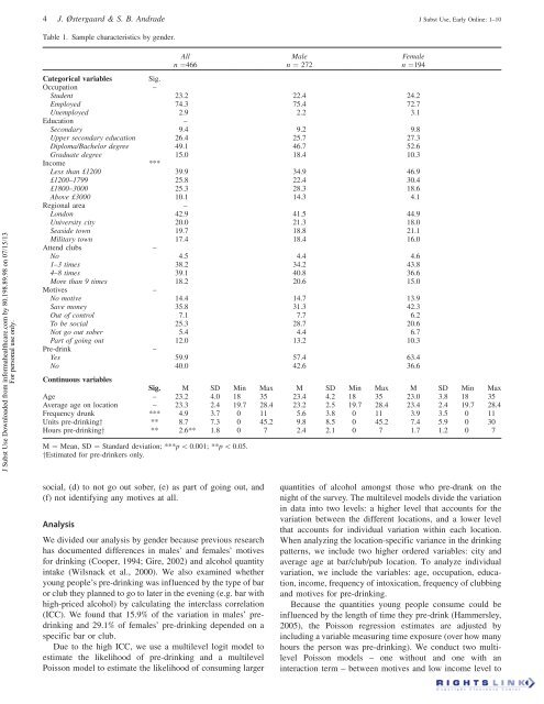
4 J. Østergaard & S. B. Andrade J Subst Use, Early Online: 1–10Table 1. Sample characteristics by gender.J Subst Use Downloaded from informahealthcare.com by 80.198.89.98 on 07/15/13For personal use only.All Male Femalen ¼466 n ¼ 272 n ¼194Categorical variables Sig.Occupation –Student 23.2 22.4 24.2Employed 74.3 75.4 72.7Unemployed 2.9 2.2 3.1Education –Secondary 9.4 9.2 9.8Upper secondary education 26.4 25.7 27.3Diploma/Bachelor degree 49.1 46.7 52.6Graduate degree 15.0 18.4 10.3Income ***Less than £1200 39.9 34.9 46.9£1200–1799 25.8 22.4 30.4£1800–3000 25.3 28.3 18.6Above £3000 10.1 14.3 4.1Regional area –London 42.9 41.5 44.9University city 20.0 21.3 18.0Seaside town 19.7 18.8 21.1Military town 17.4 18.4 16.0Attend clubs –No 4.5 4.4 4.61–3 times 38.2 34.2 43.84–8 times 39.1 40.8 36.6More than 9 times 18.2 20.6 15.0Motives –No motive 14.4 14.7 13.9Save money 35.8 31.3 42.3Out of control 7.1 7.7 6.2To be social 25.3 28.7 20.6Not go out sober 5.4 4.4 6.7Part of going out 12.0 13.2 10.3Pre-drink –Yes 59.9 57.4 63.4No 40.0 42.6 36.6Continuous variablesSig. M SD Min Max M SD Min Max M SD Min MaxAge – 23.2 4.0 18 35 23.4 4.2 18 35 23.0 3.8 18 35Average age on location – 23.3 2.4 19.7 28.4 23.2 2.5 19.7 28.4 23.4 2.4 19.7 28.4Frequency drunk *** 4.9 3.7 0 11 5.6 3.8 0 11 3.9 3.5 0 11Units pre-drinkingy ** 8.7 7.3 0 45.2 9.8 8.5 0 45.2 7.4 5.9 0 30Hours pre-drinkingy ** 2.6** 1.8 0 7 2.4 2.1 0 7 1.7 1.2 0 7M ¼ Mean, SD ¼ Standard deviation; ***p 5 0.001; **p 5 0.05.yEstimated for pre-drinkers only.social, (d) to not go out sober, (e) as part of going out, and(f) not identifying any motives at all.AnalysisWe divided our analysis by gender because previous researchhas documented differences in males’ and females’ motivesfor drinking (Cooper, 1994; Gire, 2002) and alcohol quantityintake (Wilsnack et al., 2000). We also examined whetheryoung people’s pre-drinking was influenced by the type of baror club they planned to go to later in the evening (e.g. bar withhigh-priced alcohol) by calculating the interclass correlation(ICC). We found that 15.9% of the variation in males’ predrinkingand 29.1% of females’ pre-drinking depended on aspecific bar or club.Due to the high ICC, we use a multilevel logit model toestimate the likelihood of pre-drinking and a multilevelPoisson model to estimate the likelihood of consuming largerquantities of alcohol amongst those who pre-drank on thenight of the survey. The multilevel models divide the variationin data into two levels: a higher level that accounts for thevariation between the different locations, and a lower levelthat accounts for individual variation within each location.When analyzing the location-specific variance in the drinkingpatterns, we include two higher ordered variables: city andaverage age at bar/club/pub location. To analyze individualvariation, we include the variables: age, occupation, education,income, frequency of intoxication, frequency of clubbingand motives for pre-drinking.Because the quantities young people consume could beinfluenced by the length of time they pre-drink (Hammersley,2005), the Poisson regression estimates are adjusted byincluding a variable measuring time exposure (over how manyhours the person was pre-drinking). We conduct two multilevelPoisson models – one without and one with aninteraction term – between motives and low income level to
DOI: 10.3109/14659891.2013.784368 Pre-drinking and motives 5J Subst Use Downloaded from informahealthcare.com by 80.198.89.98 on 07/15/13For personal use only.test whether the identification of lower-earning males andfemales with specific motives is associated with the consumptionof larger quantities of alcohol. We set ‘‘savingmoney’’ as the reference category for the motive variablebecause, according to previous qualitative studies (DeJong &DeRicco 2010), it is one of the main pre-drinking motives.Odds ratios (OR) and incidence rate ratios (IRR) arecalculated with Stata’s Poisson regression estimationprograme.ResultsMore males (58.4%) than females participated in the surveystudy, consistent with other bar and club studies (Hugheset al., 2007; Measham et al., 2011a; Ravn, 2010) (seeTable 1). The mean age was 23.2 years (23.4 for males and23.0 for females, t ¼ 1.00, p ¼ 0.320). Most of the youngpeople were either employed (74.3%) or students (23.2%). Anotably large percentage – 9.4% – reported having completedonly secondary education as their highest degree and 26.4%had completed or were completing upper secondary school(i.e. the education of 14-to-19-year-olds, such as A-levels andGSCS). About half (49.1%) of the interviewees had, or werecompleting, a national diploma or bachelor degree, and 15.0%were currently completing, or had completed, post-graduateschool (MA and PhD).Before taxes, 39.9% reported average earnings less than£1200 ($1850) per month. Twenty-five per cent earnedbetween £1200 and £1799 ($1850–2750), 25% earnedbetween £1800 and £3000 ($2750–4650), and only 10%earned more than £3000. Males reported significantly higheraverage monthly incomes than females (Chi ¼ 23.032, df. ¼ 3,p50.000).Amongst the young people, 62.5% reported either regularor party smoking. More than half of the 18-to-35-year-oldshad gone clubbing at least four times a month during thepreceding 30 days. The average number of times therespondents felt intoxicated during the preceding 30 dayswas 4.9, with males more likely to report intoxication thanfemales (5.6 males versus 3.9 females, t ¼ 5.02, p50.001).More than half (59.9%) of the sample had been predrinkingon the night of the interview. Amongst those whopre-drank (n ¼ 279), an average of 8.7 units of alcohol wasconsumed before a night out. Males who pre-drank had ahigher average unit consumption than females (9.80 malesversus 7.42 females, t ¼ 2.72, p50.01). Pre-drinkers beganto consume alcohol 2.1 hours before their night out, and malespre-drank for a longer period than females (2.36 h malesversus 1.68 h females, t ¼ 3.29, p50.001).The young people’s main motive for pre-drinking was‘‘saving money’’ (35.8%), a reason that more females (42.3%)than males (31.3%) reported. The second most reported motivewas ‘‘to be social’’, with which more males (28.7%) identifiedthan females (20.6%). The third motive most mentioned byboth males (14.7%) and females (13.9%) was ‘‘not identifyingwith any reason for pre-drinking’’ (either because therespondents did not see themselves as regular pre-drinkers orbecause they had no motive). Pre-drinking ‘‘to avoid going outsober’’ and ‘‘drinking to get wasted or out of control’’ was theleast common main motive for both males and females.Table 2. Results for pre-drinking (Y1). Coefficients are shown in oddsratio.MalesFemalesOR Std. OR Std.Level 2: locational variationRegional areaLondon Ref. Ref.University city 0.331** (0.169) N.S. –Seaside town N.S. – N.S. –Military town N.S. – 5.780* (0.993)Average age on location 0.692** (0.068) N.S. –Level 1: individual variationAge N.S. – 0.864** (0.037)OccupationStudent Ref. Ref.Employed 0.280** (0.126) N.S. –Unemployed N.S. – N.S. –EducationUpper secondary Ref. Ref.Diploma/Bachelor N.S. – N.S. –Graduate degree N.S. – N.S. –Secondary N.S. –IncomeLess £1200 Ref. Ref.£1200–1799 N.S. – N.S. –£1800–3000 N.S. – N.S. –Above £3000 N.S. – N.S. –Times drunk 1.092** (0.047) 1.195** (0.090)Clubbing N.S. – N.S. –Obs. 272 194Number of groups 27 27Obs. per group avg. 10.3 7.2ICC (before/after) 15.9%/40.0% 29.1%/.17.8%*p 5 0.10; **p 50.05.Table 2 shows the result of the logit multilevel models formales and females, respectively. The models estimate theinfluence of sociodemographic and socioeconomic factors onwhether males and females pre-drink before the event-specificnight. When the explanatory variables were included in themultilevel logit model, the ICC decreased from 15.9% to lessthan 0.0% for males and from 29.1% to 17.8% for females (i.e.by 38.8%). Thus, when we included a multilevel design thatcontrols for higher ordered variables, almost all locationspecificvariation disappeared for males and was reducedsignificantly for females.For males, the multilevel logit model revealed a higherordered association between age and location of bar, club andpubs, meaning that males who pre-drink before a night outattend venues where people on average are younger. It alsoshowed that students, compared to the employed, were morelikely to report pre-drinking and that for each time that themales felt intoxicated during the preceding 30 days, thelikelihood of pre-drinking also increased. Females, however,were more likely to pre-drink if they were younger, andfemales partying in the military town were more likely to predrinkthan their London counterparts. Frequent intoxicationduring the preceding 30 days also increased the likelihood offemales’ pre-drinking larger quantities before a night out.The Poisson models, shown in Table 3, estimate whethersociodemographic, socioeconomic status and pre-drinkingmotives influence how many units of alcohol, males andfemales consume when they pre-drink before an event-
Page 1 and 2: http://informahealthcare.com/jsuISS
Page 3: DOI: 10.3109/14659891.2013.784368 P
Page 7 and 8: DOI: 10.3109/14659891.2013.784368 P
Page 9 and 10: DOI: 10.3109/14659891.2013.784368 P

Who pre-drinks before a night out and why? - Alcohol Action Ireland

You also want an ePaper? Increase the reach of your titles

Delete template?

Save as template?