Lecture 9: Gaussian MAC and Broadcast channel - Multiuser ...

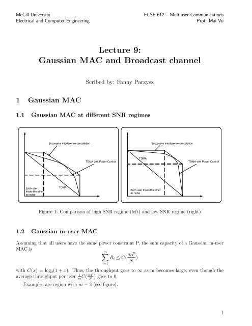
000000000000000000000000000000000000000000000000000000000000000000000000000000000000000000000000000000000000000000000000000000000000000000000000000000000000000000000000000000000000000000000000000000000000000000000000000000000000000000000000000000000000000000000000000000000000000000000000000000000000000000000000000000000000000000000000000000000000000000000000000000000000000000000000000000000000000000000000000000000000000000000000000000000000000000000000000000000000000000000000000000000000000000000000000000000000000000000000000000000000000000000000000000000000000000000000000000000000000000000000000000000000000000000000000000000000000000000000000000000000000000000000000000000000000000000000000000000000000000000000000000000000000000000000000000000000000000000000000000000000000000000000000000000000000000000000000000000000000000000000000000000000000000000000000000000000000000000000000000000000000000000000000000000000000000000000000000000000000000000000000000000000000000000000000000000000000000000000000000000000000000000000000000000000000000000000000000000000000000000000000000000000000000000000000000000000000000000000000000000000000000000000000000000000000000000000000000000000000000000000000000000000000000000000000000000000000000000000000000000000000000000000000000000000000000000000000000000000000000000000000000000000000000000000000000000000000000000000000000000000000000000000000000000000000000000000000000000000000000000000000000000000000000000000000000000000000000000000000000000000000000000000000000000000000000000000000000000000000000000000000000000000000000000000000000000000000000000000000000000000000000000000000000000000000000000000000000000000000000000000000000000000000000000000000000000000000000000000000000000000000000000000000000000000000000000000000000000000000000000000000000000000000000000000000000000000000000000000000000000000000000000000000000000000000000000000000000000000000000000000000000000000000000000000000000000000000000000000000000000000000000000000000000000000000000000000000000000000000000000000000000000000000000000000000000000000000000000000000000000000000000000000000000000000000000000000000000000000000000000000000000000000000000000000000000000000000000000000000000000000000000000000000000000000000000000000000000000000000000000000000000000000000000000000000000000000000000000000000000000000000000000000000000000000000000000000000000000000000000000000000000000000000000000000000000000000000000000000000000000000000000000000000000000000000000000000000000000000000000000000000000000000000000000000000000000000000000000000000000000000000000000000000000000000000000000000000000000000000000000000000000000000000000000000000000000000000000000000000000000000000000000000000000000000000000000000000000000000000000000000000000000000000000000000000000000000000000000000000000000000000000000000000000000000000000000000000000000000000000000000000000000000000000000000000000000000000000000000000000000000000000000000000000000000000000000000000000000000000000000000000000000000000000000000000000000000000000000000000000000000000000000000000000000000000000000000000000000000000000000000000000000000000000000000000000000000000000000000000000000000000000000000000000000000000000000000000000000000000000000000000000000000000000000000000000000000000000000000000000000000000000000000000000000000000000000000000000000000000000000000000000000000000000000000000000000000000000000000000000000000000000000000000000000000000000000000000000000000000000000000000000000000000000000000000000000000000000000000000000000000000000000000000000000000000000000000000000000000000000000000000000000000000000000000000000000000000000000000000000000000000000000000000000000000000000000000000000000000000000000000000000000000000000000000000000000000000000000000000000000000000000000000000000000000000000000000000000000000000000000000000000000000000000000000000000000000000000000000000000000000000000000000000000000000000000000000000000000000000000000000000000000000000000000000000000000000000000000000000000000000000000000000000000000000000000000000000000000000000000000000000000000000000000000000000000000000000000000000000000000000000000000000000000000000000000000000000000000000000000000000000000000000000000000000000000000000000000000000000000000000000000000000000000000000000000000000000000000000000000000000000000000000000000000000000000000000McGill UniversityElectrical and Computer EngineeringECSE 612 – Multiuser CommunicationsProf. Mai VuLecture 9:Gaussian MAC and Broadcast channelScribed by: Fanny Parzysz1 Gaussian MAC1.1 Gaussian MAC at different SNR regimesSuccessive interference cancellationSuccessive interference cancellationTDMA with Power ControlTDMATDMA with Power ControlEach usertreats the otheras noise00000000000000000000000000000000000000000000000000000000000000000000000000000TDMAEach user treats the otheras noiseFigure 1: Comparison of high SNR regime (left) and low SNR regime (right)1.2 Gaussian m-user MACAssuming that all users have the same power constraint P, the sum capacity of a Gaussian m-userMAC ism∑R i ≤ C( mPN )i=1with C(x) = log 2 (1 + x). Thus, the throughput goes to ∞ as m becomes large, even though theaverage throughput per user 1 m C(mP ) goes to 0.NExample rate region with m = 3 (see figure).1

McGill UniversityElectrical and Computer EngineeringECSE 612 – Multiuser CommunicationsProf. Mai VuR2R 1R 3Figure 2: 3-user MACZ 1 Z 2 Z rW 1Enc 1X n 11GainMatrix G1+++Y n 1Dec(W`1,W`2)X n 1rY n rW 2Enc 2X n 21GainMatrix G2X n 2r1.3 Gaussian vector-MACFigure 3: Gaussian vector MAC modelThis can modelize an OFDM, a DSL system, or a MIMO channel. We havewith Z ∼ N(0,I r ). The power constraints followY = G 1 X 1 + G 2 X 2 + Z,E[X T i · X i ] ≤ P i ⇔ tr(Σ i ) ≤ P i , i = {1, 2}Based on the same arguments as the scalar Gaussian MAC, the optimal inputs are GaussianX 1 ∼ N(0, Σ 1 ), X 2 ∼ N(0, Σ 2 ). The question is to find the optimal covariances to maximize therate region.R 1 ≤ 1 2 log det( G 1 Σ 1 G T 1 + I r)R 2 ≤ 1 2 log det( G 2 Σ 2 G T 2 + I r)R 1 + R 2 ≤ 1 2 log det( G 1 Σ 1 G T 1 + G 2 Σ 2 G T 2 + I r)2

McGill UniversityElectrical and Computer EngineeringECSE 612 – Multiuser CommunicationsProf. Mai VuIterative Waterfilling This algorithm is used to find the optimal Σ 1 and Σ 2 . User 1 performsthe single-user waterfilling algorithm considering G 2 X 2 + Z as noise. Then user 2 also performsthe single-user waterfilling algorithm, considering G 1 X 1 + Z as noise, but knowing Σ (1)1 . Next thisprocess is repeated several times. It can be proved that the iterative algorithm tends to an optimalsolution that maximizes the sum rate (R 1 + R 2 ) and converges quite fast.Iterative waterfilling is used for DSL. However, in this case, it is not a multiple access channelbut an interference channel, thus, the waterfilling solution is not optimal anymore.2 Broadcast channel (BC)2.1 DefinitionsDefinition 1 A broadcast channel is described by the set {X, p(y 1 , y 2 | x), Y 1 xY 2 }.Definition 2 A (2 nR 0, 2 nR 1, 2 nR 2, n) code consists of:• 3 message sets: M i = {1...2 nR i} for i = {0, 1, 2}• 1 encoding function: X : M 0 xM 1 xM 2 −→ X• 2 separate decoding functions: g i : Y i −→ M 0 xM i for i = {1, 2}Definition 3 The average error probability is definied byP (n)e = Pr{( ˜W 0 , ˜W1 ) ≠ (W 0 , W 1 )or ( ˜W 0 , ˜W2 ) ≠ (W 0 , W 2 )}.Definition 4 A tuple-rate (R 0 ,R 1 ,R 2 ) is achievable if P (n)eall achievable rates. In general, the capacity region for the BC is not known.−→ 0. The capacity is the closure ofn→∞2.2 TheoremThe capacity region of a BC depends only on the conditional marginal distributions p(y 1 | x) andp(y 2 | x). Thus two channels following p (1) (y 1 , y 2 | x) and p (2) (y 1 , y 2 | x) with the same marginalshave the same capacity.Sketch of the proof LetP (n)e2P (n)e1 = Pr{( ˜W 0 , ˜W1 ) ≠ (W 0 , W 1 )}P (n)e2 = Pr{( ˜W 0 , ˜W2 ) ≠ (W 0 , W 2 )}We have P e(n) ≤ P (n)e1 + P (n)e2 and max(P (n)e1 , P (n)e2 ) ≤ P e(n) , hence P e(n) −→ 0 iff P (n)e1 → 0 and→ 0. If the tuple-rate is achievable for marginals, it is also achievable for the joint distributionand vice versa.3