1 HEAT FLOW PARADOX Paradox - The seismogenic zone extends ...

z2y-V/2 V/2Q(x,z) = Vτ(z)δ(x)xThe differential equation and boundary conditions for a unit-amplitude, line source at depth -a is2 1 1∇ T =k Qxz ( , ) = δ( x) δ( z+ a) (3)kTx ( , 0)= 0lim Txz ( , ) = 0z →∞lim Txz ( , ) = 0x →∞where T is the temperature anomaly in ˚K, k is the thermal conductivity (3.3 Wm -1˚K -1 ), and Q isthe heat generation in Wm -3 . Note this is the same differential equation as equation (5) of the lastsection. The only difference is the surface boundary condition. The surface stress problem hasvanishing shear stress at the surface (i.e., vertical derivative of displacement is v is zero) so weintroduced a positive image source to force the displacement field to be symmetric about z = 0.In this heat flow case, we have vanishing temperature anomaly at the surface so we introduce anegative line heat source at z = a to form an anti-symmetric temperature function. The solutionto the full-space problem is identical to equation (14) of the previous section.[ ( ) ]Txz ( , ) = − 1ln x + z+a2πk/2 2 1 2After including the image source, the result is/ /2 2{ [ ] − [ + ( − ) ] }1 2 2 2 1 2Txz ( , ) = − 1ln x + ( z+a)ln x z a2πk(4)(5)

3Note that this is similar to equation (23) in the Turcotte et al., [1980]. The quantity of interest isthe surface heat flow versus distance from the fault./ /2 2{ [ ] − [ + ( − ) ] }1 2 2 2 1 2 (6)δqxz k T 1 δ( , ) =− = ln x + ( z+a)ln x z aδz 2πδzAfter a little algebra one arrives at the heat flow.qxz ( , ) =1 ⎧ ( z+a) ( z−a)⎨−2π⎩ x + ( z+a)x + z−a( )2 2 2 2⎫⎬⎭(7)Thus the surface heat flow for a line source of unit strength at depth a is1qx ( )=πxa+ a2 2(8)For an arbitrary shear stress distribution with depth τ(z) the surface heat flow is∞z zqx ( ) V τ=()π∫x + z dz2 2o(9)Now lets assume that the stress follows equation (1), Byerlees's law (i.e. high stress and highheat flow). Also allow hydrothermal circulation to extend from the surface to some depth dwhich effectively removes all the heat produced between the surface and that depth. Theintegration isqx ( )=2f( ρc- ρw) gVzπ∫x + z dz2 2Dd(10)This integral is done with help from the table of integrals.∫2xa bx dx x a 1= -b b a bx dx2 2+∫(11)+After some algebra one arrives at the following analytic formula for the heat flowf( ρc- ρw) gV⎧d Dqx ( ) = ( D−d) ⎛ −1 −1xtan − x tan⎞ ⎫⎨ +⎩ ⎝ x x ⎠⎬(12)π⎭It is interesting to compare this heat flux to the heat flux at a mid-ocean ridge for the same totalopening rate V (see figure on next page). The formula is

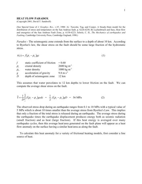
4qx ( ) kT ( T) 2πκx/V (13)= − ( )mo-1/2Τ m mantle temperature 1600 ˚KΤ o surface temperature 273 ˚Kk thermal conductivity-13.3 Wm-1˚Kκ thermal diffusivity 8. x 10 -7 m 2 s -1Matlab ExampleThe following is a Matlab program simulates a high-stress fault (i.e., Byerlee's Law)extending to a depth of 12 km and sliding at a rate of 30 mm/yr. Two cases are considered; thefirst case (solid curve on next page) has hydrothermal heat removal extending to a depth of 1 kmwhile the second (dotted curve) has heat removal to a depth of 5 km. These models arecompared with the heat flow measurements across the San Andreas Fault [Lachenbruch andSass, 1980]. It is clear that the shallow heat removal model is inconsistent with the data.However, the deep heat removal model is not precluded by the observations, especially if thebackground level of the model heat flow is allowed to vary from the spatial average. Oneargument against hydrothermal removal of heat is the absence of hot springs along the fault withsufficient vigor to remove this heat. Hydrothermal circulation is the dominant heat removalmechanism at the mid-ocean ridges and hydrothermal vents are common. However, as shown inthe following figure, heat generation along a strike-slip fault is 2-3 orders of magnitude less thana mid-ocean ridge so it is not clear that the same mechanism should operate at a fault. Even ifheat loss is concentrated in small areas it may be difficult to detect at the surface.%% program to calculate the surface heat flux due to frictional heating on a% strike-slip faultD=12;d1=1; d5=5;rc=2600; rw=1000; g=9.8;V=.03/3.15e7; f=.60;q0=1.e6*f*(rc-rw)*g*V/pi;%% calculate the heat flow for the two models of shallow and deep heat removal%x=-60:.1:60;q1=q0*((D-d1)+x.*atan(d1./x)-x.*atan(D./x));q5=q0*((D-d5)+x.*atan(d5./x)-x.*atan(D./x));% plot the resultsplot(x,q1+73,x,q5+73,':');xlabel('distance (km)'); ylabel('heat flow (mWm-2)')axis([-120,120,0,167]);

140120-2heat flow (mWm )100806040200100 50 0 50 100distance (km)10 4 distance (km)-2heat flow (mWm )10 210 0mid-ocean ridgestrike-slip fault60 40 20 0 20 40 60

6MOMENT PARADOX: Seismic Moment versus Tectonic Saturation MomentThe Moment Paradox described next is really part of the heat-flow paradox except it isexpressed in a different way. As discussed in a previous lecture, and in Brace and Kohlstedt[1980], measurements of stress difference in the uppermost crust to depths of several kilometersare consistent with a yield strength model following Byerlee's law. The static frictionalresistance to sliding is related to a coefficient of friction f of about 0.60 times the overburdenpressure of ∆ρgz. This leads to differential stress difference of 140 MPa at a depth of only 10km. We also found that these high stresses are required to support the 5000 m elevation of Tibetrelative to India. This isostatic model is the minimum stress needed to support topography so itis clear that high stresses exist at shallow depths in the crust. Similarly, one can calculate thebending moment needed to support the trench and outer rise topography at a subduction zone.The moment calculation is model-independent [ McNutt and Menard, Constraints on yieldstrength in the oceanic lithosphere derived from observations of flexure, Geophs. J. R. astr. Soc.,71, p. 363-394, 1982;]Mx ( )/ L= ∆ρ wx ( ) x−x dx(1)o∞∫x o( )owhere M is the moment per unit length along the trench, ∆ρ is the mantle-to-seawater densitycontrast, is the height of the outer rise above the normal depth and x-x o is the distance betweenthe first zero crossing of the trench flexure profile and some point out on the outer rise. Theintegral converges because w(x) goes to zero exponentially with distance. Observed bendingmoments at outer rises vary from 5 x 10 16 N for young lithosphere (10 Ma) to 3 x 10 17 at oldoceanic lithosphere (140 Ma) [Levitt and Sandwell, Lithospheric bending at subduction zonesbased on depth soundings and satellite gravity, J. Geophys. Res., 100, p. 379-400, 1995]. Nextwe'll compare these numbers to typical seismic moments of large earthquakes using the Alaska1964 and Landers 1992 event as examples. The Landers rupture was about 70 km long so we'lldivide its moment by length for the comparison with models. The results are provided in thetable below.

7tectonic examplemoment per length (N)outer rise flexure (10 Ma)5 x 10 16 Nouter rise flexure (140 Ma) 3 x 10 17 NAlaska flexure1.2 x 10 17 NAlaska 1964 earthquake, M9.2 1.1 x 10 17 N = 8.2 x 10 22 /750 kmLanders 1992 earthquake, M7.4 1.4 x 10 15 N geodetic/length2.8 x 10 15 N seismic/lengthByerlee's criterion (0 - 12 km only) 1.3 x 10 16 N mThis comparison highlights two issues: first, the moment of the Alaska 1964 earthquake wassufficient to cause a collapse of the outer rise(??); second, the seismic/geodetic moment of theLanders 1992 earthquake is 10-20 times smaller than the moment estimated next using a thesimple elastic dislocation model where stress is limited only by Byerlee's law.Seismic Moment Released During an EarthquakeL yxDzThe moment released during an earthquake can be estimated in two ways, either by analysisof the seismic radiation pattern or by the geodetic analysis of the geodetic ground motion. Theyusually provide similar values; although in the case of the Landers 1992 rupture, the seismicmoment estimate is about 2 times the geodetic moment estimate. The moment is defined asM = µ sLD ∆ y(2)f static coefficient of friction ~ 0.60ρ c crustal density 2600 kg m -3ρ w water density 1000 kg m -3g acceleration of gravity 9.8 m s -2µ shear modulus 2.6 x 10 10 PaL length of rupture 70 kmD depth of rupture 12 km

There are only two ways to understand this delemma.A) Faults are somehow lubricated (f~.05) so the average stress on the fault is 10-20 timessmaller than predicted by Byerlee's law. In this case one has the difficulty of maintaining theelevation of the topography in California. For example, San Jacinto Mountain, which is less than25 km from the San Andreas Fault, has a relief of about 3000 m which implies stresses of 80MPa (16 times the stress drop in an earthquake).B) Faults are strong as predicted by Byerlee's law. In this case, faults are always very close tofailure and each earthquake relieves only a small fraction (~10%) of the tectonic stress. As wesaw in the last section, this model implies a large amount of energy dissipation along the fault;friction from both aseismic creep and seismic rupture will generate heat. It has been proposedthat perhaps during the earthquake, the coefficient of friction drops from 0.60 to say 0.05 totemporarily disable the heat generation. However, is seems that such a slippery fault wouldrelease all of the elastic energy during an earthquake (~60 m of offset). Another possibility isthat heat is generated but a large fraction of the heat is advected to the surface by circulation ofwater in the upper couple km of crust. The unfortunate implication of this high-stress model isthat since faults are always close to failure, it will be almost impossible to predict earthquakes.9