Lesson Fifteen. More Linear Algebra - Department of Mathematics ...

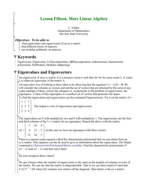
Lesson Fifteen. More Linear AlgebraL. ValdesDepartment of MathematicsSan Jose State UniversityObjectives: To be able to1. find eigenvalues and eigenvectors of an nx n matrix2. find different forms of matrices3. use modular arithmetic on matricesKeywordsEigenvector, Eigenvalue, LUDecomposition, QRDecomposition, orthornormal, characteristicpolynomial, DotProduct, Modular subpackageEigenvalues and EigenvectorsAn eigenvector of an nx n matrix A is a nonzero vector v such that Av=λv for some scalar λ. A scalarλ is called an eigenvalue of the matrix A.An equivalent way of looking at these ideas is by observing that the equation A Kγ I v = 0. Wewill consider the columns as vectors and call the set of vectors that are obtained by the sums of anyscalar multiple of these vectors the subspace or, in particular to the problem of eigenvectors, theeigenspace. A basis of this eigenspace is a smallest set of vectors that generates the space.To find the eigenvalues and eigenvectors use the command Eigenvectors(). Try it on the matrix A1=1 1 12 2 5. The output is a list of eigenvalues and eigenvectors.3 3 6The eigenvalues are 0 with multiplicity two and 9 with multiplicity 1. The eigenvectors are the firstand third columns of the 3 x 3 matrix for an eigenspace. Repeat the above with the matrixK7 K16 4A2 =6 13 K212 16 1. In this case we have an eigenspace with three vectors.There is a special scalar equaion called the characteristic polynomial that we can obtain from annx n matrix. This equation can the be used to give us information about the eigenvalues. The Maplecommand is CharacteristicPolynomial(Matrix,variable). Find the characteristic polynomials ofA1 Kλ I and A2 Kλ I and then solve them.Do you recognize these values?We get a bonus when the number of eigenvectors is the same as the number of columns or rows ofthe matrix. We can say that the matrix is diagonalizable. That is we can find a matrix P such thatP A2 P K1 = D2 where D2 contains zero entries off the diagonal. That matrix is the nx n matrix

eturned yielding the eigenvectors. Assign that matrix above to the name E and determineE K1 .A2.E. Assign this output the name D2. Do you recognize the entries?Suppose you had to find A2 100 . Well, Maple can do that, but the computation is equivalent toA2 10 = E.D2.E K1 10 = E.D2 10 .E K1 . A power, i, of a diagonal matrix is especially easy to determine -it is simply the ith power of each of the diagonal entries. Find A 10 and E.D 10 .E K1 below.Standard Forms of MatricesThere are various standard forms of matrices. We have already considered Gaussian elimination andthe upper triangular form it takes and the reduced echelon form. We can also rewrite a matrix as aproduct of two matrices. One such form is called the LU factorization. The matrix L is invertibleand is called a unit lower triangular matrix and U is an upper triangular matrix in echelon form. Thecommand is LUDecomposition(Matrix). Try it on A2. Then try assigning the output to p, l, and uwhere p is a permutation matrix, l is the lower and u is the upper matrix in the factorization. Finally,multiply the three matrices.If the dot product of two vectors equals zero and the dot product of the vectors with themselves311equals one, we call the vectors orthonormal. Prove to yourself that the two vectors u =111111K 1 6and v =2616are orthonormal. Use the command DotProduct.A QR Factorization of an mx nmatrix A is a product QR where Q is an mx n matrix with orthonormalcolumns and R is an nx n upper triangular invertible matrix with positive diagonal entries. Thecommand is QRDecomposition(Matrix). Find the QR decomposition of the matrix A3. Find the dotproduct of column 1 with itself.The last standard form we will be studying is called the Jordan canonical form. We say twomatrices A and B are similar if there exists an invertible matrix P such that A = P K1 .B.P. Any matrixis similar to a matrix in Jordan canonical form. Use the command JordanForm on the matrices A1and A2. The form is not always a diagonal matrix. Check back to where you found the eigenvectorsof the two matrices and determine when there were only two eigenvectors and when there was one.

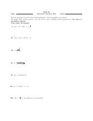
More practice. Find the characteristic polynomial of A4:=form of A4. Finally find the eigenvectors.Modular Linear Algebra3 1 K2K1 0 5K1 K1 4, factor it, find the JordanMaple also allows us to work with matrices modulo n. We need to open the subpackage of theLinearAlgebra package called Modular. To do so type with(LinearAlgebra[Modular]).There are several ways in which you can create a matrix in mod n. For our purposes, we willconstruct our matrices as in Lesson Fourteen and then "mod out" by n if necessary. That is, if theentries are not in the range 0 ..n K1, then we will use the Mod(modulus,MatrixName,integer). Use it1 K9 10on the matrix M1 =3 K10 4with modulus = 5 and give it the new name M2.K88 K6Another convenient way to create matrices is with the command Random(modulus,rows,columns,integer). Create a 3 x 3 matrix modulus and call it M3.Now that we know how to construct matrices, let us learn how to use the basic operations ofaddition, multiplication, finding the inverse, transpose, and determinant. The command AddMultiple(n,A,B) returns the sum of the matrices A and B modulus n. The command AddMultiple(n,k,A,B)returns A+kB modulus n. Try both of these on M2 and M3.To multiply two matrices use Multiply(modulus,A,B). Try it on M2 and M3. Then try it on M1 andM3.To find the inverse use Inverse(modulus,A). Find the inverse of M2, call it M4 and then find theproduct of M2 and M4. Find the inverse of M3.To find the determinant and transpose use Determinant(modulus,Matrix) and Transpose(modulus,Matrix). Try the commands below.The characteristic polynomial is of special interest when using modular arithmetic. To find it, useCharacteristicPolynomial(modulus,expression,variable). Find the characteristic polynomial of M2,call it a, and then use factor(a) to factor it.It apparently is not factorable. However, what if we wish to factor it mod 5? Then try Factor(a) mod5 and call the output b.Use expand(b) and try to determine if you understand this last result.