Smooth functional tempering for nonlinear differential equation models

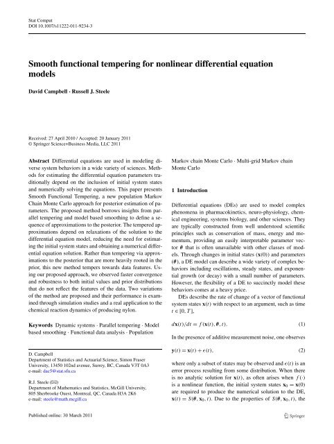
Stat ComputDOI 10.1007/s11222-011-9234-3Smooth functional tempering for nonlinear differential equationmodelsDavid Campbell · Russell J. SteeleReceived: 27 April 2010 / Accepted: 20 January 2011© Springer Science+Business Media, LLC 2011Abstract Differential equations are used in modeling diversesystem behaviors in a wide variety of sciences. Methodsfor estimating the differential equation parameters traditionallydepend on the inclusion of initial system statesand numerically solving the equations. This paper presentsSmooth Functional Tempering, a new population MarkovChain Monte Carlo approach for posterior estimation of parameters.The proposed method borrows insights from paralleltempering and model based smoothing to define a sequenceof approximations to the posterior. The tempered approximationsdepend on relaxations of the solution to thedifferential equation model, reducing the need for estimatingthe initial system states and obtaining a numerical differentialequation solution. Rather than tempering via approximationsto the posterior that are more heavily rooted in theprior, this new method tempers towards data features. Usingour proposed approach, we observed faster convergenceand robustness to both initial values and prior distributionsthat do not reflect the features of the data. Two variationsof the method are proposed and their performance is examinedthrough simulation studies and a real application to thechemical reaction dynamics of producing nylon.Keywords Dynamic systems · Parallel tempering · Modelbased smoothing · Functional data analysis · PopulationD. CampbellDepartment of Statistics and Actuarial Science, Simon FraserUniversity, 13450 102nd avenue, Surrey, BC, Canada V3T 0A3e-mail: dac5@stat.sfu.caR.J. Steele ()Department of Mathematics and Statistics, McGill University,805 Sherbrooke Ouest, Montreal, QC, Canada H3A 2K6e-mail: steele@math.mcgill.caMarkov chain Monte Carlo · Multi-grid Markov chainMonte Carlo1 IntroductionDifferential equations (DEs) are used to model complexphenomena in pharmacokinetics, neuro-physiology, chemicalengineering, systems biology, and other sciences. Theyare typically constructed from well understood scientificprinciples such as conservation of mass, energy and momentum,providing an easily interpretable parameter vectorθ that is often unavailable with other classes of models.Through changes in initial states (x(0)) and parameters(θ), a DE model can describe a wide variety of complex behaviorsincluding oscillations, steady states, and exponentialgrowth (or decay) with a small number of parameters.However, the flexibility of a DE to succinctly model thesebehaviors comes at a heavy price.DEs describe the rate of change of a vector of functionalsystem states x(t) with respect to an argument, such as timet ∈[0,T],dx(t)/dt = f(x(t), θ,t). (1)In the presence of additive measurement noise, one observesy(t) = x(t) + ɛ(t), (2)where only a subset of states may be observed and ɛ(t) is anerror process resulting from some distribution. When thereis no analytic solution for x(t), as often arises when f(·)is a nonlinear function, the initial system states x 0 = x(0)are required to produce the numerical solution to the DE,x(t) = S(θ, x 0 ,t). Due to the properties of S(θ, x 0 ,t),the

Stat Computlikelihood for y(t) in (2) may be rife with undesirable topographysuch as local maxima, ridges, ripples and/or largeflat segments (Esposito and Floudas 2000). We will primarilyfocus on ordinary differential equations (ODEs) in ourwork.There is a rich literature in the biological sciencesproposing solutions to the parameter estimation problemfor models like (1). Varah (1982) and Voit and Sauvegeau(1982) first proposed the use of smoothing for the estimationof the parameters of an ODE. Ramsay and Silverman(2005) and Poyton et al. (2006) extended Varah’s approachto iterate between smoothing the data and estimating theparameters of the underlying ODE. A recent approach toparameter estimation based on generalized profiling (GP)also aims to improve the likelihood topology by using adata smooth ˆx(t) ≈ S(θ, x 0 ,t) resulting from a basis expansion.Estimates of θ are determined by the profile likelihood,marginalizing over the nuisance parameters used toconstruct ˆx(t) (Ramsay et al. 2007). Data smoothing usingGP accounts for both the dynamics in (1) and the datafeatures, providing an increased basin of attraction for themode of θ. Smoothing removes the dependence on the nuisanceparameters x 0 and improves stability of the estimateof θ. However, it has been shown that a profile likelihood approachcan perform poorly in the presence of multiple nuisanceparameters (Walley and Moral 1999). Additionally,a purely frequentist approach does not allow for valuableprior information about the system to be incorporated intothe modeling.We present a new Bayesian sampling method for posteriorestimation of θ and x 0 (if desired) from ODE models.The proposed smooth functional tempering (SFT) is apopulation Markov Chain Monte Carlo (MCMC) methodthat uses the GP model as a bridging auxiliary density ina parallel tempering algorithm (PT). Our approach employsa GP data smooth to define a sequence of approximationsto the posterior with increased basins of attraction for themodes. SFT does not require a priori knowledge of the posteriortopology or a bounded posterior space. Furthermore,unlike previous implementations of PT, SFT is robust to situationswhere prior information is inconsistent with the data.We propose two variations on our technique, one that incorporatesthe initial conditions in the estimation (SFT1)and a more computationally efficient alternative approachwhich profiles over the initial conditions, reducing the dimensionalityof the parameter space (SFT2). Section 2 reviewsbackground methods and leads into the description ofboth proposed variants of SFT in Sect. 3. A simulation studyis given in Sect. 4 which examines the performance of ourapproaches in a canonical example from the statistical ODEliterature. We conclude with a real data case study in Sect. 5and a discussion of our results (Sect. 6).2 BackgroundThe lack of an analytical form for S(θ, x 0 ,t) implies thatthere is no closed form for the likelihood. Gradient basedmethods like non-linear least squares (NLS) do not typicallyperform well and practitioners are warned to expecta method based error level of the order of 25%(Bates and Watts 1988; Marlin 2000). New evolutionaryapproaches to maximization of the likelihood function areable to overcome many of these shortcomings, althoughinference depends on asymptotic approximations for standarderrors or computationally expensive bootstrap procedures(Rodriguez-Fernandez et al. 2006; Miaoetal.2009;Liang and Wu 2008; Liang et al. 2010). Bayesian modelsprovide an alternative to asymptotic frequentist analysis ofODE data. Typical Bayesian parameter estimation methodsfor ODEs (for two examples, see Gelman et al. 1996or Huang and Wu 2006) use a model of the form:y(t) | θ, x 0 ,σ 2 ∼ N ( S(θ, x 0 ,t),σ 2) ,θ, x 0 ,σ 2 ∼ P(θ, x 0 ,σ 2 ).A Bayesian approach for ODEs requires Monte Carlosimulation or numerical integration, and most implementationsof Bayesian ODE models have used MCMC methods.For example, Barenco et al. (2006) and Rogers et al. (2007)both used traditional Metropolis sampling methods to obtainBayesian posterior estimates for ODE parameters usedfor predicting gene transcription activity. Klinke (2009) implementedan adaptive MCMC approach for Bayesian estimationof a complex signaling network. The GNU MC-Sim software (Bois 2009) allows for Bayesian estimation ofODE models coded in Systems Biology Markup Language(SBML). However, current applications of MCMC requirethat the ODE is numerically solved at each proposed parametervalue which makes exploration of the posterior surfaceunder these topological difficulties challenging. Examplesof these kinds of problems are shown in Sect. 4.2. Simulatedannealing has been used to circumvent the topological difficulties(Gonzalez et al. 2007), but still requires a numericalsolution to the ODE at each iteration. The dependence onS(θ, x 0 ,t) also increases the dimensionality of the parameterspace with the inclusion of x 0 , a set of nuisance parametersthat grows in dimension with additional experimentalruns. The structural parameters, θ, are of primary interestbecause they define the ODE dynamics, yet current methodstreat x 0 , θ and σ 2 in (3) equally, despite their differinginfluence on the data-generating process and importance inestimation.The primary challenges for Bayesian ODE estimationmethods are that the topology of the posterior and location ofthe dominant mode are difficult to determine, the likelihood(and, thus, the un-normalized posterior distribution) generallydoes not have a closed form expression, and the param-(3)

Stat ComputFig. 1 A cross section of the FitzHugh-Nagumo log likelihood for γ (bottom) and the fits to the data for V (grey)andR (black) corresponding tothe likelihood modes using the true parameter values (top middle), a small value (top left) and a large value (top right)eter space may be unbounded and high dimensional. Furthermore,the posterior surface may have local maxima surroundedby deep and wide likelihood valleys making determiningthe global mode difficult. Figure 1 shows an exampleof a multimodal posterior surface where local modes associatedwith a partial fit to the data are of negligible posteriorrelevance. Therefore, a Bayesian approach to ODE modelsrequires a method that can adeptly manage these challengingfeatures.The nature of the posterior topology for difficult modelsis often referred to in the biological literature as “sloppiness”.In statistics, the term normally used would be “nonidentifiable”or, if not strictly not identifiable, then onlyweakly identifiable with respect to estimating parametersfrom the observed data. The wide extent of the sloppinessin biological systems problems is discussed in a paperby Gutenkunst et al. (2007b), where they identify sloppinessissues with parameters in a large number of modelsextracted from the BioModels database (Le Novère etal. 2006). There is a large amount of work that has beendone to develop methods for identifying problems that aresloppy in nature and to choose parameterizations that remedythe problem (Gutenkunst et al. 2007a; Vilela et al. 2007;Raue et al. 2009). The body of work on identifying and remedyingsloppy parameterizations is interesting and could bepotentially used in conjunction with our approach to improveinference, but it is beyond the scope of our work here.2.1 Population MCMCPopulation based simulation methods are designed to improvemobility of MCMC samplers using information fromparallel MCMC chains based on a sequence of approximationsto the posterior density. Parallel tempering (PT), forexample, approximates the posterior distribution of ψ =[θ, x 0 ] through a sequence of m = 1,...,M approximations;P m (ψ | y) ≈ P(ψ | y) defined by a temperature gradient0 ≤ ξ 1 < ···

Stat ComputFig. 2 The effect of changingthe temperature gradientparameter on the-log(-log(non-normalizedposterior)) for methods(columns) using different priorsfor γ (rows). Increasing valuesof the parameter (ξ for PT, λ forSFT1 and SFT2) gives linesappearing lower down withineach plotthe M chains are not generated entirely independently. Withsome probability, two chains k and l are randomly selectedand their parameters ψ (i)kand ψ (i)lare proposed to be exchangedbetween the chains rather than mutate independently.The exchange is accepted with probabilityr swap = min(1, P k(ψ (i)l| y)P l (ψ (i)P k (ψ (i)kk| y)| y)P l (ψ (i)l| y)Over time, the proposed exchanges between neighboringchains should be accepted approximately 50% of the timeto ensure reasonably smooth sequence of distributions (Liu2001). The exchange step enables multiple modes to be sampledand improves mixing for the chain sampling from theposterior of interest, P(ψ | y).Parallel tempering and genetic algorithms (GA) sharemany conceptual similarities. The critical difference betweenthe two approaches is that parallel tempering is usedfor generating samples from a distribution rather than for optimizationof an objective function (Liang and Wong 2000).Parallel tempering allows for two kinds of updates to themodel parameters, mutation steps (the MH updates performedwithin each chain) and exchange (the MH updatesperformed between chains). In their work, Liang and Wong(2000, 2001) also suggested a potential crossover (knownas recombination in the GA literature in optimization research)move that would allow for only portions of the parametervector to be exchanged between chains. However,this crossover move can be difficult to implement in practiceand so we have not used it as part of our simulations. Fora comprehensive and somewhat current review of the literatureon these methods, we encourage the readers to see Jasraet al. (2007).PT and variants (Marinari and Parisi 1992; Neal 1996;Calderhead et al. 2009) have been shown to work well forsampling from certain multi-modal densities. However, despiteenabling the sampler to escape local posterior modes,).the posterior flattening strategies that improve the mobilityof some parameters may over-flatten parameter dimensionswith less complex posterior topologies leading to slowermixing and burn-in in the target distribution (Geyer andThompson 1995). Additionally since tempering is almost alwaysdone towards the prior, PT will fail when prior informationdoes not agree with the features of the observed data(see Sect. 4.2).2.2 Model-based smoothingModel-based smoothing is a generalization of smoothingsplines or penalized smoothing (Eilers and Marx 1996).The mean of the data is assumed to be a linear combinationof basis functions (φ(t)) with coefficients (c), i.e.E[y(t)]=x(t) = c ′ φ(t). The shape of the smooth dependson the hyper-parameter λ and can be expressed as a distributionon x(t),P(x(t) | θ,λ)∝ exp[− λ ]2 PEN(x, θ,t)where∫ [ dx(s)2PEN(x, θ,t)= − f (x(s),θ,s)]ds. (5)t dsA Bayesian extension of this model would then assume afurther prior distribution for (θ,λ,σ 2 )A standard choice in the smoothing literature for thepenalty term is PEN = ∫ t (d2 x(s)/ds 2 − 0) 2 ds. This definesa model structure that anticipates a linear model, whereasin (5), the penalty is more generally based on the integratedsquare of the residual of (1). When used as a kernel for aprior on x(t), we see that the prior density increases as x(t)approaches the shape defined by the ODE model throughPEN. Model parameters θ from (1) can be considered ashyper-parameters of the prior on x(t).

Stat ComputThe smoothing parameter λ defines a balance betweenmeasurement error σ 2 and deviation from the ODE model.As λ → 0, the posterior mode of x(t) | y, θ,σ 2 ,λ is thefunction space spanned by the basis that interpolates thedata. As λ →∞, the posterior mode of x(t) | y, θ,σ 2 ,λoccurson the function space spanned by the ODE solution.Model-based smoothing was not designed for optimal estimationof θ when the parametric structure of (1) isassumed.To highlight this, note that λ controls the flow ofinformation between y and θ because θ is conditionally independentof y given x(t), λ, and σ 2 . Consequently, modelbased smoothing reduces the impact of changes in θ on x(t),inflating var(θ | y) compared to estimating θ via (3) withoutthe hierarchical layer of the data smooth.In some cases x 0 may be known to high precision, butremaining trajectory x(t, x 0 ) must be estimated. These initialvalue problems generally could be computed using constrainedoptimization, however the computation is simplifiedusing a B-spline basis since there is only one basis functiontaking a non-zero value at each of the time interval boundaries.With respect to parameter estimation, if x 0 is known,this additional information can improve reliability in the estimationof θ, especially when the model is sensitive to initialconditions (Wu et al. 2008).3 Smooth functional tempering (SFT)Our novel approach to Bayesian estimation of ODE models,Smooth Functional Tempering (SFT), is a particularform of parallel tempering, as it is defined by a sequenceof M distributions towards the posterior of the measurementerror model in (3). However, SFT is best seen asa collocation tempering method that uses the data-smoothas an auxiliary distribution. SFT depends on a basis expansionfor the approximation x(t) = c ′ φ(t) ≈ S(θ, x 0 ,t)and tempers towards the posterior by varying the smoothingparameter. When using a B-spline basis, as the smoothingparameter increases and the ODE model is more rigorouslyenforced, x(t) → S(θ, x 0 ,t), where x 0 = c ′ φ(t = 0)and S(θ, x 0 ,t) is numerically computed using an implicitRunge-Kutta method with stepping points at the knot locations(Deuflhard and Bornemann 2000). Consequently, basingthe tempering process on a collocation method is equivalentto basing the tempered chains on a relaxation to theODE solution. In this section, we outline two variations ofthis process. The first variation (SFT1) employs a smoothapproximation to the initial value problem and utilizes afixed point in the data smoothing step in conjunction with anumerical ODE solution. The second variation (SFT2) usessmooth approximations and does not depend on numericalODE solutions or x 0 .3.1 SFT1: parameter estimation with a smooth and anumerical ODE solutionWe first assume that we are interested in making inferenceabout x 0 and/or the function space spanned by the possibleODE solutions as well as θ. SFT1 defines a tempering strategytowards model (3) based on the increasing sequence offixed smoothing parameters 0

Stat Computnumerical solution may be difficult to produce or may besubject to propagating numerical errors due to the relianceon x 0 . SFT2 avoids the potential liability of numericallysolving the ODE and eliminates the need to explicitly modelx 0 by tempering via the sequence of distributions for 0

Stat Computshape of S(θ, x 0 ,t) and transformed to the parameter space[θ, x 0 ]. Non-informative or loosely informative (vague) priorson the parameter space may lead to prior distributionsthat are quite informative on the function space (see,for example, Salway and Wakefield 2008; Wakefield 1996;Wakefield and Bennett 1996; and Bates and Watts 1988).One could, for example, place a bounded, piece-wise constantset of uniform priors over regions of the functionspace where there is confidence the function values mustlie. Then one can use a (potentially non-linear) transformationto transform this vague prior distribution on the functionspace to a prior over the parameters of the model (Salwayand Wakefield 2008). In practice, working entirely witha prior distribution on the function space (for example, usinga Gaussian process prior) is often easier to specify andmanage computationally than transforming distributions onfunction spaces into priors on θ. However, the challengethen shifts to relating posterior inference on the functionspace to the underlying parameters of the ODE (Gao et al.2008) A formal comparison between these two approachesis beyond the scope of this paper.4 Simulated examples from the FitzHugh-NagumomodelThe FitzHugh-Nagumo differential equations (FitzHugh1961; Nagumo et al. 1962) comprise a simple model forthe voltage potential across the cell membrane of the axonof giant squid neurons. These equations are used in neurophysiologyas an approximation of the observed spike potential.The voltage V moving across the cell membrane dependson the recovery variable R through the relationship:dVdtdRdt= γ(V − V 3 )3 + R ,=− 1 γ (V − α + βR) . (8)An example of a simulated data set and the true underlyingprocess when γ = 3 appears in Fig. 1. Figure 1 alsoincludes a cross section of the log likelihood and additionalODE solutions using parameter values corresponding to minormodes of the cross section. The mode corresponding tovalues of γ ≈ 0.5 produces a ODE solution with the correctperiod but the shape is too sinusoidal to represent thedynamics of V . The likelihood mode corresponding to valuesof γ ≈ 9 produces approximately the correct shape butdoes not match the period. Traversing the likelihood surfacein either direction from the local modes causes a deteriorationin the data fit before it can be improved. Anysampling or optimization algorithm would encounter wideregions of prohibitively deep posterior topology of approximately4000 units deep on the log scale. We consider a particularone-parameter version of this model, where all parametersother than γ are held fixed, in order to highlight theability to accurately estimate the posterior in Sect. 4.1. Wehave set the fixed parameters to values that yield a bimodallikelihood surface that is representative of the types of irregularitiesthat are observed in problems involving ODEs.We compare Bayesian and frequentist methods using theone dimensional version of this model in Sect. 4.2. ThefullFitzHugh-Nagumo model, where all unknown parametersare estimated, is explored in Sect. 4.3. A simulation examiningcomputational effort in a real data setting is saved forSect. 5.1.4.1 One dimensional bimodal exampleIn this section we alter (8) to produce a symmetric, bimodalposterior for γ ;dVdtdRdt=|γ |(V − V 3 )3 + R ,=− 1|γ | (V − α + βR) . (9)Due to the computational intensity of working with differentialequations, we restricted ourselves to ten simulateddata sets, obtained from the numerical solution to (9) usingthe parameter γ = 3 at the 201 evenly spaced time pointst = 0, 0.1, 0.2,...,20 with added Gaussian white noise. Focusingattention on γ , all other parameters are held fixed attheir true values (α = 0.2, β = 0.2, σ 2 V = 0.25, σ 2 R = 0.16,V 0 =−1, and R 0 = 1) so that the posterior density canbe evaluated numerically and compared with results fromSFT1, SFT2 and PT under two different prior distributions:P(γ)= 1 2 χ 2 2 , γ >0P(−γ)= 1 2 χ 2 2 , γ

Stat ComputFig. 3 Discrepancy betweensampled and numerical posteriorestimates using different priordistributions and samplingmethods. Boxplots show D( P) ˆusing the uniform prior (left)and the χ 2 based prior (right)Fig. 4 The autocorrelationfunctions for the SFT1 (solidline), SFT2 (dotted line)andPT(dashed line) for the bimodalproblem of Sect. 4.1,withtheuniform prior (left)andtheχ 2based prior (right). The heavylines are the point-wise meanautocorrelation functionsFor each of the two prior distributions for γ , the numericallyevaluated posterior (P num ) was compared with the resultsof the sampling based methods using the IntegratedSquared Error (ISE):∫ [ ] 2D( Pˆsampled ) = P num (γ | y) − Pˆsampled (γ | y) dγ.(12)The ISE values are shown in Fig. 3 for the M th chains usingthe last 40,000 posterior draws after discarding burn-in.For comparison, note that the M th chains of SFT1 andPT use the same target distribution. In our simulations, PTperformed somewhat better than SFT1 when using a uniformprior on γ but somewhat worse with a χ 2 based prior,although both performed well based on the ISE. SFT1 andPT both use the true value of x 0 , but SFT2 estimates γ withoutthis additional knowledge. Consequently, SFT2 uses lessinformation than the other two approaches, leading to a posteriorvariance around the modes (at γ =±3), which is approximately7 times wider than that using SFT1 or PT. In orderto make for a fair comparison, D( PˆSFT 2 ) was computedcomparing the sampled density with the numerical estimateof its smooth based density from the M th chain.Figure 4 shows the autocorrelation functions (ACFs) andtheir point-wise mean ACFs for the posterior samples of theλ M chains. The main factor dominating the ACF is the exchangebetween the modes at ±3. SFT2 performs the bestwith respect to this criterion, in part due to the lack of dependenceon the initial conditions. SFT1 generally ranks second,likely due to the reduced impact of initial conditions inthe finite λ m parallel chains. The ACFs for PT are slowestto decay. We do not observe an impact of the choice of priordistribution on the ordering of the ACFs in this example.4.2 Inconsistent prior informationIn this section, we focus on the one dimensional problemof estimating P(γ | y) using the FitzHugh-Nagumo model(8) with a prior that is inconsistent with the observed data:γ ∼ N(14, 2 2 ). The bottom row of Fig. 2 shows that theglobal mode of the target posterior at γ = 3 remains virtuallyunchanged by this change in prior. Parameter estimationwas attempted using SFT1, SFT2, PT, single chainMetropolis Hastings (MH), NLS and GP on 10 data setsfrom the measurement error model from Sect. 4. SFT1 andSFT2 were performed with 6 parallel chains each and PTwas equipped with 10. All chains in all methods were initializedat γ = 10. The number of burn-in iterations determinedby the Raftery-Lewis criterion (Raftery and Lewis 1992)was less than 125 in all cases from this starting point. Afterdiscarding 1,000 iterations, both the Raftery-Lewis and

Stat ComputFig. 5 Boxplots of theestimates of γ in Sect. 4.2,thedashed line is where themethods where initialized, thetrue parameter value is 3. Top:Estimates for all 6 methods,bottom, rescaled to show detailGeweke convergence diagnostics (Geweke 1992) indicateconvergence from all of the independent chains from all thesampling methods.Figure 5 shows a boxplot of the final parameter estimates.MH and NLS are not able to escape the strong gradient towardsthe local mode at γ = 12. The strategy of temperingtowards the prior hindered any of the PT chains from findingthe global mode because the smaller λ chains enforcebehavior inconsistent with the data features and emphasizethe local mode at γ = 12 within the alloted 100,000 iterations.Both SFT1 and SFT2 used the increased basin of attractionof their smaller λ-valued parallel chains and temperingtowards data features to avoid the impact of the inconsistentprior information. GP also smoothes the likelihood towardsthe data features and the point estimate converged quicklyclose to the true value. Since x 0 is assumed known, SFT1uses this additional information to perform better than SFT2and GP.4.3 FitzHugh-Nagumo, full modelWhile the previous simulations showed the ability of themethods to produce reasonable results in a single dimension,the performance of SFT2 was negatively impacted becauseit did not use information about the initial conditions. In thissection, we use model (8) with simulated data from the morerealistic scenario where no parameters are known. Prior distributionsfor θ = (γ,α,β)were determined by numericallysolving the ODE over a coarse grid of values of θ and placingapproximately 95% of the prior mass over the values thatproduce oscillatory dynamics giving:γ ∼ χ 2 2 , P(α)= P(β)= N(0, 0.42 ) (13)Priors for x 0 = (V 0 ,R 0 ) were chosen based on the observeddata, where the priors for both were chosen to be independentGaussian densities centered on the first observedvalue with variance equal to the observed data variance,which places most of the prior mass in regions where datafor V and R were actually observed. The priors for the varianceparameters σV 2 and σ R 2 were chosen to be Jeffreys, i.e.P(σV,R 2 ) ∝ 1/σ V,R 2 . In this simulation study we used 30 differentdata sets, each with 401 evenly spaced observationsfor each of V and R. This large amount of data ensured thatthe likelihood was well approximated by a multivariate Normaldistribution, making the Delta method interval estimatesof Ramsay et al. (2007) good approximations.For these simulations we focus on SFT1, SFT2 and GPbecause of the bad performance of PT for the inconsistentprior distribution in Sect. 4.2. Parameters were initializedwith draws from the prior. All parallel chains (across allmethods) were initialized with the same values. SFT1 andSFT2 used 4 parallel chains and GP was performed usingan increasing sequence of λ values as suggested in Ramsayet al. (2007) such that SFT2 and GP have the same value ofλ M =10,000. The point estimates are shown in Fig. 6 basedon 30,000 posterior draws after burn-in. The observed magnitudeof the bias is small and there are no significant differencesin performance amongst the methods in this example.

Stat ComputFig. 6 Bias in point estimatesfor the FitzHugh-Nagumoparameters α (top), β (middle)and γ (bottom) of Sect. 4.35 Nylon exampleIn this section, we model the production of nylon in a heatedreactor where its constituents, amine (A) and carboxyl (C),combine to produce the polymer, nylon (L), and water (W),which escapes as steam. At the same time, before escapingthe system as steam, W decomposes L into A and C in themolten nylon mixture, giving the symbolic competing reactionsA + C ⇋ L + W . In the experiment of Zheng et al.(2005), steam is bubbled through molten nylon to maintainan approximately constant concentration of W in the systemcausing A, C and L to move towards equilibrium concentrationswith W. Within each of the i = 1,...,6 experimentalruns, the pressure of input steam was held at a high level untiltime τ i1 , and then reduced until time τ i2 , at which point itreturned to its original level for the remainder of the experiment.Each experiment was performed at a constant temperatureT i which, along with the input water pressure, determinesthe equilibrium concentration of water in the moltennylon mixture, W eq . Using reaction rates k p and K a , the dynamicsof the model are described with the following systemof differential equations:− dL = dA = dC =−k p (CA − LW/K a )10 −3 , (14)dt dt dtdW= k p 10 −3 (CA − LW/K a ) − 24.3(W − W eq ). (15)dtThe reaction rate K a is allowed to change with T i andW eq through relationships depending on the reference temperatureT 0 = 549.15 giving four ODE parameters: θ =[k p ,γ,K a0 ,H] by the following expansion of K a :{K a = 1 + W eq γ 10 −3} ( HK T [K a0 ]l8.314), (16){ 1l(m) = exp(−m10 3 − 1 }), (17)T i T 0(K T = 20.97 exp −9.624 + 3613 ). (18)T iFigure 7 shows the data for each of the 6 experimentalruns. The plot shows the observed components A and C aswell as input W eq . Due to the mass balance of this system,given any three components the fourth can be computed exactly.Because only A and C are observed, we must estimatethe unobserved W(t) for each experimental run. Furthermore,since the components are chemical reactions, theyare constrained to take on non-negative values. In the nylonsystem, x 0 increases the dimension of the parameter spacefrom 6 parameters in [θ,σ 2 ], to 24 parameters; [θ, x 0 ,σ 2 ].We set our prior distribution to be uniform on the set offunctions taking values between 0 and 250, where 250 wasselected because it its about 10% larger than the largest observation.We chose this interval to be wider than is likely tobe necessary to place non-zero mass over realistic functionsfor this problem. It is likely that values of the unobservedW would remain close to the values of W eq (all take onvalue less than 100) but the more conservative value of 250was used throughout for the states A, C and W . Additionally,the prior distributions on 1/σA 2 and 1/σ C 2 were chosento be independent Gamma densities with mean 9 and variance27. These are pessimistic priors relative to the measurementerror variance estimates from additional experimentsby Zheng et al. (2005).We implemented SFT1 and SFT2 using evenly spacedknots placed at a rate of 3 per hour of experimental duration.In anticipation of sharp dynamics after the step change in inputW eq , an additional 9 knots were evenly spaced at timesτ +[0.1, 0.2,...,0.9] after the input change. The discontinuousfirst derivative induced by the step input change wasaccommodated by the addition of knots at the time of thestep change. SFT2 was implemented with values λ 1 = 100,and λ 2 = 10, 000. SFT1 required four times the number ofparameters of the SFT2 model and consequently M = 3chains were used, with tempering values λ 1 = 200,λ 2 =500.

Stat ComputFig. 7 The nylon observations along with the fit to the data. Temperatures of the experimental runs are given above component A in degreesKelvin. Vertical axes are in concentration units and horizontal axes are in hoursFig. 8 A comparison of theposterior density estimates forthe nylon parameters usingSFT1 (black line) and SFT2(dashed line)The small values of λ 1 in both methods produced considerablerobustness with respect to values used to initializethe Markov Chains. The kernel density estimate of 40,000posterior draws from the M th chain of SFT1 and SFT2 forθ,σA 2 and σ C 2 (after discarding burn-in) are shown in Fig. 8.Estimates for the marginal posterior densities of θ are similarbetween the methods, and the values for the integratedsquared difference between marginal posteriors comparingSFT1 with SFT2 are 0.057, 0.016, 0.018 and 0.0073 fork p0 , γ,K a0 and H respectively. The squared discrepancybetween the marginal posterior density estimates deviatesslightly more for σA 2 and σ C 2 giving values equal to 0.11 and0.15 respectively. The reason for this discrepancy may lie inthe marginal posterior density estimates of x 0 , estimated bySFT1 and shown in Fig. 9. The dynamics of the system arequite fast, so that the impact for some of the experimentalruns on moving W 0 from near 0 to near 250 only affects thefit to the first few data points, leading to some relatively flat(and uninformative) posterior distributions. SFT1 exploresthe distribution of X 0 and, in the process, finds more valuesthat allow a better fit to A in exchange for a decrease in fit toC giving the shifted densities for σC 2 and σ A 2 showninFig.8.SFT1 also allows for new insights into the vast uncertaintyin W 0 . The advantages of SFT2 are the reduced dimensionof the problem and, in this case, a five fold computationaltime reduction.5.1 Comparison of computational effortThe simulation studies of Sect. 4 were performed with highresolution, homoscedastic data from a fully observed systemin order to highlight the algorithmic performance inthe face of specific posterior topological difficulties. Datasuch as this are unlikely to be observed often in practice.In this section, we examine the variability in computationtime of the SFT1, SFT2 and PT algorithms using more realisticreplications of the same algorithmic process wherethe only difference between algorithmic trials is the randomseed initializations. This is in contrast to the simulation studiesof Sect. 4 where each trial used a different random dataset. Variability in the computation time required for a singleiteration of the sampler depends on the parameter valuesbeing proposed because they determine the stiffness (magnitudeof the derivative) of the differential equation system.When numerically solving an ODE, a stiff system is considerablyslower than a non-stiff system and the parametervalues determine the stiffness (Deuflhard and Bornemann2000). Consequently, we use repeated algorithmic simulationson a fixed real dataset to compare the algorithmic differencesin methods and examine the practical advantages ofthe proposed methods.The full nylon model in (14)–(18) requires multiple experimentalruns to estimate the temperature dependency ofk p and K a , however for this study we use a single experimentalrun of the nylon dataset, (shown in Fig. 7 with tem-

Stat ComputFig. 9 Histograms of posteriordraws x 0 in the nylon systemusing SFT1. Rows are for thedifferent experimental runs,while columns are (left to right)A 0 , C 0 and W 0perature of 544), performed at a fixed temperature. Consequently,we use the model (14) and (15) without further expansionof k p and K a . The priors from Sect. 5 were re-usedto produce the statistical model.The algorithmic study was run with this unevenly spacedpartially observed data set 50 times for each of the threemethods compared. Each of the 50 algorithmic simulationsper method were run for 50,000 iterations from the samestarting point and the computational time and effective samplesize were measured after discarding the first 10,000 forburn in.The within chain ODE parameters, [k p ,K a ,A 0 ,C 0 ,W 0 ]for PT and SFT1 or [k p ,K a ] for SFT2 were updated in asingle step using Metropolis Hastings tuned with the optimalnormal jumping kernel. Variance terms were updatedusing Gibbs steps. The 3 methods were attempted with 3parallel chains each where λ and ξ values were chosen to obtainan acceptance rate of 50% between neighboring chains.Each method required the same number of evaluations ofPEN(·) per iteration. Although distributed computing is naturalwhen dealing with population MCMC, all runs were allottedonly a single 3 GHz processor core with 1 Gb RAM.The compute time, effective sample size and ratio thereofare shown in Fig. 10. While PT was about 30% faster on average,13 of the 50 PT trials proposed at least one set of stiffparameters such that the stiff Runge-Kutta solver, ode15sin Matlab® (The MathWorks 2010), failed to solve the ODEwithin the permitted numerical tolerance bounds. Breakingthe solver in this way was much faster than actually solvingthe system at these numerical limits.The autocorrelation differences in Fig. 4 were primarilydue to the SFT algorithms’ ability to jump between distantmodes, whereas here the target posterior is unimodal, reducingthe advantage of SFT1 over PT. Figure 10 shows thatSFT1 and PT effective sample sizes are less than half thatof SFT2. Consequently, SFT2 results in a large advantage interms of the compute time per independent draw, shown inthe right of Fig. 10 and defined as the average over relevantparameters A,C,k p ,K a ,A 0 ,C 0 ,W 0 of:Total compute time for 40,000 iterationsEffective Sample Size from those 40,000 iterations .6 DiscussionParameter estimation for nonlinear differential equationspresents challenges for both frequentist and Bayesian modelingwhere, despite the appearance of convergence, the likelihoodtopology may not permit either convergence to orsampling around the global optima. Our proposed SFT approachesutilize model based smoothing to construct auxiliarydensities for PT to match the features of the datawith the dynamics of the model and improve estimation.This variation of tempering smooths out the posterior enablingfaster convergence towards the dominant mode, andas such, represents an important new tool for populationbasedMCMC simulation. While the simulations and applicationpresented feature nonlinear differential equationmodels, the methods are applicable to nonlinear regressionin general, especially when the response surface is prohibitive.SFT1 and SFT2 temper towards the data featuresto improve posterior mobility, whereas PT was shown to failwhen tempering towards a prior that is inconsistent with thedata. Using SFT, priors can therefore be used to describeknowledge about the system without needing to also accountfor it’s utility in providing an adequate tempering strategy.

Stat ComputFig. 10 Summary ofcomputational effort for SFT1,SFT2, and PT. Left to right:totalcompute time, effective samplesize, compute time perapproximate independentposterior sample for the 2parameter nylon simulationIn the presence of prior information consistent with thedata features, SFT1, SFT2 and PT perform similarly, as measuredby integrated squared error discrepancy between simulatedand numerical posterior estimates. However SFT hasthe advantage of reduced dependence on initial conditionswhich can reduce the autocorrelation between samples.When the likelihood and posterior were unimodal, SFT1,SFT2 and GP produced similar point estimates. Given additionalinformation in the form of x 0 , SFT1 was able toout-perform both of these methods, even with a prior thatwas inconsistent with the data. In the case of multi-modality,GP requires additional information to find additional modes,whereas SFT methods were shown to be successful in theFitzHugh-Nagumo bimodal example with only 10 parallelchains in an example where the posterior consisted of twowidely separated modes.It is rarely the case that a computational approach willuniversally provide improvement, as one can always constructexamples where a particular method can fail. Ourwork has shown that the SFT approaches can significantlyimprove upon the usual implementation of the PT algorithmin certain situations without yielding significantly worseperformance in situations where the standard PT approachperforms well. The SFT2 approach, which avoids dependenceon the initial system states (x 0 ), performs very welland is significantly computationally less intensive per independentsample than the other approaches, especially whenthe ODE is computationally slow to solve.Our objective in this paper was to propose a bettercomputational approach to Bayesian analysis of nonlineardifferential equation models. There exist many promisingnon-Bayesian solutions to this problem, particularly inthe field of biology. Varah (1982) and Voit and Sauvegeau(1982) both proposed a data-smoothing approach toestimate the parameters of an ODE. More modern workin this area includes the use of artificial neural networksto estimate parameters in a non-parametric way (Voit andAlmeida 2004). Chou and Voit (2009) provide a fairly comprehensiveoverview of not only different potential solutionsfor estimation of model parameters, but also for differentapproaches to specification of the model and generalissues with these types of non-linear biological systems.Brunel (2008) explores the asymptotics of combining nonparametricsmoothing with parameter estimation for datagenerated from non-linear ODE’s and provides a new twostepapproach that seems promising.Similarly, although we have chosen a particular type ofsmoother, i.e. the generalized profiling method (Ramsay etal. 2007), as an auxiliary density, one would not be restrictedto using only this kind of smoother. Other potential smoothingauxiliary models could be used, such as the perfectsmoother of Eilers (2003) or the adaptation of Whitaker’ssmoother proposed by Vilela et al. (2007). We have used thegeneralized profiling method because of our familiarity withthe smoother and the ease with which one can interpret thesingle smoothing parameter as a temperature in the temperingprocess. Other choices for the smoother could performeither better or worse (likely depending on the particulardata problem) and we hope to explore this in future work.It would be interesting to see whether an ensemble of differentchoices of smoother would be computationally feasibleas well.Producing a data smooth to the ODE is not necessarilya computational improvement compared to producinga numerical solution to a ODE model. When the ODE isstiff, however, computing a numerical solution can alreadybe extremely computationally intensive (Huang et al. 2006;Li et al. 2002) and using a relaxation of the numerical solutioncan accelerate iterations and convergence. The useof parallel processing reduces the total computational timeof the population MCMC method and ensures minimal additionalcomputational time from adding additional chains.To further reduce the computational load in SFT, one couldomit computing x(t) or x(t, x 0 ) at each proposed value andinstead update only occasionally during mutation step, whileupdating always at the exchange steps. The success of thismodification to our algorithm depends strongly on the qualityof the smooth approximation to the ODE model and the

Stat Computsensitivity of the dynamics to the parameters. This modificationwill certainly alter the effectiveness of the posteriorsampling, although it is not clear exactly how. We thus leavethe subject to future investigation.There may be some interest in a mixed dimension approachthat implements SFT2 along with an additional parallelchain using the model (3), where for some l

Stat ComputGramacy, R., Samworth, R., King, R.: Importance tempering. Stat.Comput. 20, 1–7 (2010)Gutenkunst, R.N., Casey, F.P., Waterfall, J.J., Myers, C.R., Sethna, J.P.:Extracting falsifiable predictions from sloppy models. Ann. N.Y.Acad. Sci. 1115, 203–211 (2007a)Gutenkunst, R.N., Waterfall, J.J., Casey, F.P., Brown, K.S., Myers,C.R., Sethna, J.P.: Universally sloppy parameter sensitivities insystems biology models. PLoS Comput. Biol. 3, 1871–1878(2007b)Huang, Y., Liu, D., Wu, H.: Hierarchical Bayesian methods for estimationof parameters in a longitudinal HIV dynamic system. Biometrics62, 413–423 (2006)Huang, Y., Wu, H.: A bayesian approach for estimating antiviral efficacyin HIV dynamic models. J. Appl. Stat. 33, 155–174 (2006)Jasra, A., Stephens, D.A., Holmes, C.C.: On population-based simulationfor static inference. Stat. Comput. 17, 263–279 (2007)Kass, R.E., Raftery, A.: Bayes factors. J. Am. Stat. Assoc. 90(430),773–795 (1995)Klinke, D.J.: An empirical Bayesian approach for model-based inferenceof cellular signaling networks. BMC Bioinform. 10, 371(2009)Le Novère, N., Bornstein, B., Broicher, A., Courtot, M., Donizelli, M.,Dharuri, H., Li, L., Sauro, H., Schilstra, M., Shapiro, B., Snoep,J., Hucka, M.: BioModels database: a free, centralized databaseof curated, published, quantitative kinetic models of biochemicaland cellular systems. Nucleic Acids Res. 34(Suppl 1), D689–D691 (2006)Li, L., Brown, M.B., Lee, K.H., Gupta, S.: Estimation and inference fora spline-enhanced population pharmacokinetic model. Biometrics58, 601–611 (2002)Liang, F., Wong, W.: Evolutionary Monte Carlo sampling: applicationsto Cp model sampling and change-point problem. Stat. Sin. 10,317–342 (2000)Liang, F., Wong, W.H.: Real-parameter evolutionary Monte Carlo withapplications to Bayesian mixture models. J. Am. Stat. Assoc. 96,653–666 (2001)Liang, H., Miao, H., Wu, H.: Estimation of constant and time-varyingdynamic parameters of HIV infection in a nonlinear differentialequation model. Ann. Appl. Stat. 4, 460–483 (2010)Liang, H., Wu, H.: Parameter estimation for differential equation modelsusing a framework of measurement error in regression models.J. Am. Stat. Assoc. 103, 1570–1583 (2008)Liu, Jun S.: Monte Carlo strategies in Scientific Computing. Springer,New York (2001)Marinari, E., Parisi, G.: Simulated tempering: a new Monte Carloscheme. Europhys. Lett. 19, 451–458 (1992)Marlin, T.E.: Process Control. McGraw-Hill, New York (2000)The MathWorks: Matlab ®7 Mathematics. The Mathworks, Inc. Natick,MA (2010)Miao, H., Dykes, C., Demeter, L.M., Wu, H., Avenue, E., York, N.,York, N.: Differential equation modeling of HIV viral fitness experiments:model identification, model selection, and multimodelinference. Biometrics 65, 292–300 (2009)Nagumo, J.S., Arimoto, S., Yoshizawa, S.: An active pulse transmissionline simulating a nerve axon. Proc. Inst. Radio Eng. 50,2061–2070 (1962)Neal, R.M.: Sampling from multimodal distributions using temperedtransitions. Stat. Comput. 4, 353–366 (1996)Olhede, S.: Discussion on the paper by Ramsay, Hooker, Campbell andCao. J. R. Stat. Soc. B 69, 772–779 (2008)Poyton, A., Varziri, M., McAuley, K., McLellan, P., Ramsay, J.: Parameterestimation in continuous-time dynamic models using principaldifferential analysis. Comput. Chem. Eng. 30, 698–708(2006)Qi, X., Zhao, H.: Asymptotic efficiency and finite-sample propertiesof the generalized profiling estimation of parameters in ordinarydifferential equations. Ann. Stat. 38(1), 435–481 (2010)Raftery, A., Lewis, S.: How many iterations in the Gibbs sampler. In:Bernardo, J.M., Berger, J.O., Dawid, A.P., Smith, A.F.M. (eds.)Bayesian Statistics. Proceedings of the Fourth Valencia InternationalMeeting, vol. 4, pp. 763–773. Clarendon Press, Oxford(1992)Ramsay, J.O., Hooker, G., Campbell, D., Cao, J.: Parameter estimationfor differential equations: a generalized smoothing approach (withdiscussion). J. R. Stat. Soc. B 69, 741–796 (2007)Ramsay, J.O., Silverman, B.W.: Functional Data Analysis. Springer,New York (2005)Raue, A., Kreutz, C., Maiwald, T., Bachmann, J., Schilling, M., Klingmüller,U., Timmer, J.: Structural and practical identifiability analysisof partially observed dynamical models by exploiting the profilelikelihood. Bioinformatics 25, 1923–1929 (2009)Rodriguez-Fernandez, M., Mendes, P., Banga, J.R.: A hybrid approachfor efficient and robust parameter estimation in biochemical pathways.Biosystems 83, 248–65 (2006)Rogers, S., Khanin, R., Girolami, M.: Bayesian model-based inferenceof transcription factor activity. BMC Bioinform. 8, S2 (2007)Salway, R., Wakefield, J.: Gamma generalized linear models for pharmacokineticdata. Biometrics 64, 620–626 (2008)Varah, J.: A spline least squares method for numerical parameter estimationin differential equations. SIAM J. Sci. Stat. Comput. 3,28–46 (1982)Vilela, M., Borges, C.C.H., Vinga, S., Vasconcelos, A.T.R., Santos, H.,Voit, E.O., Almeida, J.S.: Automated smoother for the numericaldecoupling of dynamics models. BMC Bioinform. 8, 305 (2007)Voit, E.O., Almeida, J.: Decoupling dynamical systems for pathwayidentification from metabolic profiles. Bioinformatics 20, 1670–1681 (2004)Voit, E.O., Sauvegeau, M.: Power-law approach to modeling biologicalsystems; III. Methods of analysis. J. Ferment. Technol. 60, 233–241 (1982)Walley, P., Moral, S.: Upper probabilities based only on the likelihoodfunction. J. R. Stat. Soc. B 61, 831–847 (1999)Wakefield, J.: The Bayesian analysis of population pharmacokineticmodels.J.Am.Stat.Assoc.91, 62–75 (1996)Wakefield, J., Bennett, J.: The Bayesian modeling of covariates forpopulation pharmacokinetic models. J. Am. Stat. Assoc. 91, 917–927 (1996)Wu, H., Zhu, H., Miao, H., Perelson, A.S.: Parameter identifiabilityand estimation of HIV/AIDS dynamic models. Bull. Math. Biol.70, 785–799 (2008)Zheng, W., McAuley, K.B., Marchildon, E.K., Zhen Yao, K.: Effectsof end-group balance on melt-phase nylon 612 polycondensation:experimental study and mathematical model. Ind. Eng. Chem.Res. 44, 2675–2686 (2005)