Smooth functional tempering for nonlinear differential equation models

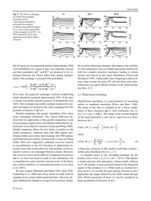
Stat ComputFig. 2 The effect of changingthe temperature gradientparameter on the-log(-log(non-normalizedposterior)) for methods(columns) using different priorsfor γ (rows). Increasing valuesof the parameter (ξ for PT, λ forSFT1 and SFT2) gives linesappearing lower down withineach plotthe M chains are not generated entirely independently. Withsome probability, two chains k and l are randomly selectedand their parameters ψ (i)kand ψ (i)lare proposed to be exchangedbetween the chains rather than mutate independently.The exchange is accepted with probabilityr swap = min(1, P k(ψ (i)l| y)P l (ψ (i)P k (ψ (i)kk| y)| y)P l (ψ (i)l| y)Over time, the proposed exchanges between neighboringchains should be accepted approximately 50% of the timeto ensure reasonably smooth sequence of distributions (Liu2001). The exchange step enables multiple modes to be sampledand improves mixing for the chain sampling from theposterior of interest, P(ψ | y).Parallel tempering and genetic algorithms (GA) sharemany conceptual similarities. The critical difference betweenthe two approaches is that parallel tempering is usedfor generating samples from a distribution rather than for optimizationof an objective function (Liang and Wong 2000).Parallel tempering allows for two kinds of updates to themodel parameters, mutation steps (the MH updates performedwithin each chain) and exchange (the MH updatesperformed between chains). In their work, Liang and Wong(2000, 2001) also suggested a potential crossover (knownas recombination in the GA literature in optimization research)move that would allow for only portions of the parametervector to be exchanged between chains. However,this crossover move can be difficult to implement in practiceand so we have not used it as part of our simulations. Fora comprehensive and somewhat current review of the literatureon these methods, we encourage the readers to see Jasraet al. (2007).PT and variants (Marinari and Parisi 1992; Neal 1996;Calderhead et al. 2009) have been shown to work well forsampling from certain multi-modal densities. However, despiteenabling the sampler to escape local posterior modes,).the posterior flattening strategies that improve the mobilityof some parameters may over-flatten parameter dimensionswith less complex posterior topologies leading to slowermixing and burn-in in the target distribution (Geyer andThompson 1995). Additionally since tempering is almost alwaysdone towards the prior, PT will fail when prior informationdoes not agree with the features of the observed data(see Sect. 4.2).2.2 Model-based smoothingModel-based smoothing is a generalization of smoothingsplines or penalized smoothing (Eilers and Marx 1996).The mean of the data is assumed to be a linear combinationof basis functions (φ(t)) with coefficients (c), i.e.E[y(t)]=x(t) = c ′ φ(t). The shape of the smooth dependson the hyper-parameter λ and can be expressed as a distributionon x(t),P(x(t) | θ,λ)∝ exp[− λ ]2 PEN(x, θ,t)where∫ [ dx(s)2PEN(x, θ,t)= − f (x(s),θ,s)]ds. (5)t dsA Bayesian extension of this model would then assume afurther prior distribution for (θ,λ,σ 2 )A standard choice in the smoothing literature for thepenalty term is PEN = ∫ t (d2 x(s)/ds 2 − 0) 2 ds. This definesa model structure that anticipates a linear model, whereasin (5), the penalty is more generally based on the integratedsquare of the residual of (1). When used as a kernel for aprior on x(t), we see that the prior density increases as x(t)approaches the shape defined by the ODE model throughPEN. Model parameters θ from (1) can be considered ashyper-parameters of the prior on x(t).