Smooth functional tempering for nonlinear differential equation models

More documents

Recommendations

Info

Stat ComputFig. 2 The effect of changingthe temperature gradientparameter on the-log(-log(non-normalizedposterior)) for methods(columns) using different priorsfor γ (rows). Increasing valuesof the parameter (ξ for PT, λ forSFT1 and SFT2) gives linesappearing lower down withineach plotthe M chains are not generated entirely independently. Withsome probability, two chains k and l are randomly selectedand their parameters ψ (i)kand ψ (i)lare proposed to be exchangedbetween the chains rather than mutate independently.The exchange is accepted with probabilityr swap = min(1, P k(ψ (i)l| y)P l (ψ (i)P k (ψ (i)kk| y)| y)P l (ψ (i)l| y)Over time, the proposed exchanges between neighboringchains should be accepted approximately 50% of the timeto ensure reasonably smooth sequence of distributions (Liu2001). The exchange step enables multiple modes to be sampledand improves mixing for the chain sampling from theposterior of interest, P(ψ | y).Parallel tempering and genetic algorithms (GA) sharemany conceptual similarities. The critical difference betweenthe two approaches is that parallel tempering is usedfor generating samples from a distribution rather than for optimizationof an objective function (Liang and Wong 2000).Parallel tempering allows for two kinds of updates to themodel parameters, mutation steps (the MH updates performedwithin each chain) and exchange (the MH updatesperformed between chains). In their work, Liang and Wong(2000, 2001) also suggested a potential crossover (knownas recombination in the GA literature in optimization research)move that would allow for only portions of the parametervector to be exchanged between chains. However,this crossover move can be difficult to implement in practiceand so we have not used it as part of our simulations. Fora comprehensive and somewhat current review of the literatureon these methods, we encourage the readers to see Jasraet al. (2007).PT and variants (Marinari and Parisi 1992; Neal 1996;Calderhead et al. 2009) have been shown to work well forsampling from certain multi-modal densities. However, despiteenabling the sampler to escape local posterior modes,).the posterior flattening strategies that improve the mobilityof some parameters may over-flatten parameter dimensionswith less complex posterior topologies leading to slowermixing and burn-in in the target distribution (Geyer andThompson 1995). Additionally since tempering is almost alwaysdone towards the prior, PT will fail when prior informationdoes not agree with the features of the observed data(see Sect. 4.2).2.2 Model-based smoothingModel-based smoothing is a generalization of smoothingsplines or penalized smoothing (Eilers and Marx 1996).The mean of the data is assumed to be a linear combinationof basis functions (φ(t)) with coefficients (c), i.e.E[y(t)]=x(t) = c ′ φ(t). The shape of the smooth dependson the hyper-parameter λ and can be expressed as a distributionon x(t),P(x(t) | θ,λ)∝ exp[− λ ]2 PEN(x, θ,t)where∫ [ dx(s)2PEN(x, θ,t)= − f (x(s),θ,s)]ds. (5)t dsA Bayesian extension of this model would then assume afurther prior distribution for (θ,λ,σ 2 )A standard choice in the smoothing literature for thepenalty term is PEN = ∫ t (d2 x(s)/ds 2 − 0) 2 ds. This definesa model structure that anticipates a linear model, whereasin (5), the penalty is more generally based on the integratedsquare of the residual of (1). When used as a kernel for aprior on x(t), we see that the prior density increases as x(t)approaches the shape defined by the ODE model throughPEN. Model parameters θ from (1) can be considered ashyper-parameters of the prior on x(t).
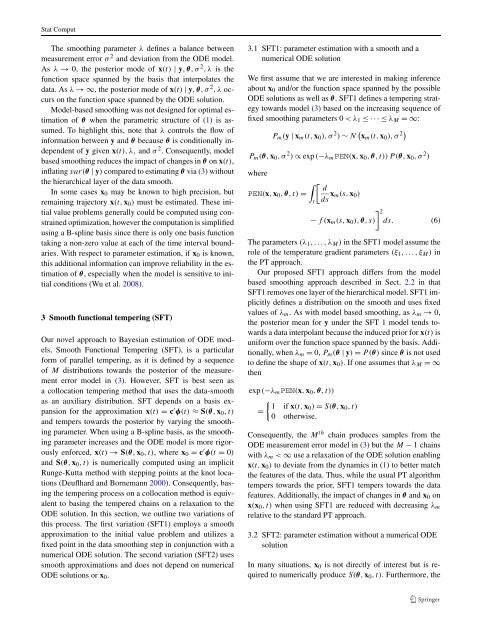
Stat ComputThe smoothing parameter λ defines a balance betweenmeasurement error σ 2 and deviation from the ODE model.As λ → 0, the posterior mode of x(t) | y, θ,σ 2 ,λ is thefunction space spanned by the basis that interpolates thedata. As λ →∞, the posterior mode of x(t) | y, θ,σ 2 ,λoccurson the function space spanned by the ODE solution.Model-based smoothing was not designed for optimal estimationof θ when the parametric structure of (1) isassumed.To highlight this, note that λ controls the flow ofinformation between y and θ because θ is conditionally independentof y given x(t), λ, and σ 2 . Consequently, modelbased smoothing reduces the impact of changes in θ on x(t),inflating var(θ | y) compared to estimating θ via (3) withoutthe hierarchical layer of the data smooth.In some cases x 0 may be known to high precision, butremaining trajectory x(t, x 0 ) must be estimated. These initialvalue problems generally could be computed using constrainedoptimization, however the computation is simplifiedusing a B-spline basis since there is only one basis functiontaking a non-zero value at each of the time interval boundaries.With respect to parameter estimation, if x 0 is known,this additional information can improve reliability in the estimationof θ, especially when the model is sensitive to initialconditions (Wu et al. 2008).3 Smooth functional tempering (SFT)Our novel approach to Bayesian estimation of ODE models,Smooth Functional Tempering (SFT), is a particularform of parallel tempering, as it is defined by a sequenceof M distributions towards the posterior of the measurementerror model in (3). However, SFT is best seen asa collocation tempering method that uses the data-smoothas an auxiliary distribution. SFT depends on a basis expansionfor the approximation x(t) = c ′ φ(t) ≈ S(θ, x 0 ,t)and tempers towards the posterior by varying the smoothingparameter. When using a B-spline basis, as the smoothingparameter increases and the ODE model is more rigorouslyenforced, x(t) → S(θ, x 0 ,t), where x 0 = c ′ φ(t = 0)and S(θ, x 0 ,t) is numerically computed using an implicitRunge-Kutta method with stepping points at the knot locations(Deuflhard and Bornemann 2000). Consequently, basingthe tempering process on a collocation method is equivalentto basing the tempered chains on a relaxation to theODE solution. In this section, we outline two variations ofthis process. The first variation (SFT1) employs a smoothapproximation to the initial value problem and utilizes afixed point in the data smoothing step in conjunction with anumerical ODE solution. The second variation (SFT2) usessmooth approximations and does not depend on numericalODE solutions or x 0 .3.1 SFT1: parameter estimation with a smooth and anumerical ODE solutionWe first assume that we are interested in making inferenceabout x 0 and/or the function space spanned by the possibleODE solutions as well as θ. SFT1 defines a tempering strategytowards model (3) based on the increasing sequence offixed smoothing parameters 0
Page 1 and 2: Stat ComputDOI 10.1007/s11222-011-9
Page 3: Stat ComputFig. 1 A cross section o
Page 7 and 8: Stat Computshape of S(θ, x 0 ,t) a
Page 9 and 10: Stat ComputFig. 5 Boxplots of thees
Page 11 and 12: Stat ComputFig. 7 The nylon observa
Page 13 and 14: Stat ComputFig. 10 Summary ofcomput
Page 15: Stat ComputGramacy, R., Samworth, R

Smooth functional tempering for nonlinear differential equation models

Create successful ePaper yourself

Delete template?

Save as template?