Continuous quantum measurement of two coupled quantum dots ...

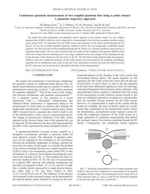
GOAN, MILBURN, WISEMAN, AND SUN PHYSICAL REVIEW B 63 125326The form of the master equation 7, defined through thesuperoperator DB(t), preserves the positivity of the densitymatrix operator (t). Such a Markovian master equationis called a Lindblad 50 form.To demonstrate the equivalence between the master equation7 and the rate equations derived in Ref. 16, we evaluatethe density matrix operator in the same basis as in Ref. 16and obtain˙ aa ti ab t ba t,˙ ab ti ab ti aa t bb tX T 2 /2 ab ti ImT *X T *X ab t.13a13bHere ( 2 1 ) is the energy mismatch between thetwo dots, ij (t)i(t) j, and aa (t) and bb (t) are theprobabilities of finding the electron in dot 1 and dot 2, respectively.The rate equations for the other two density matrixelements can be easily obtained from the relations: bb (t)1 aa (t) and ba (t) ab* (t). Compared to an isolatedCQD system, the presence of the PC detector introducestwo effects to the CQD system. First, the imaginarypart of the product of T *X T *X the last term in Eq.13b causes an effective temperature-independent shift inthe energy mismatch between the two dots. Here (T *X T *X T *X )T*X is a temperature-independent quantitywhere TT (0), i.e., T and X evaluated at zero temperature,respectively. Second, it generates a decoherencedephasing rate d X T 2 /214for the off-diagonal density matrix elements, where X T 2X 2 X 2 . We note that the decoherence rate comesentirely from the effect of the measurement revealing wherethe electron in the CQD’s is located. If the PC detector doesnot distinguish which of the dots the electron occupies, i.e.,X 0, then d 0. The rate equations in Eq. 13 are exactlythe same as the zero-temperature rate equations in Ref.16 if we assume that the tunneling amplitudes are real, T 00T 00* and 00 00* . In that case, the last term in Eq. 13bvanishes and d X 2 /2(DD) 2 /2. Actually, the relativephase between the two complex tunneling amplitudesmay produce additional effects on conditional dynamics ofthe CQD system as well. This will be shown later when wediscuss conditional dynamics. Physically, the presence of theelectron in dot 1 raises the effective tunneling barrier of thePC due to electrostatic repulsion. As a consequence, the effectivetunneling amplitude becomes lower, i.e., DTX 2 DT 2 . This sets a condition on the relative phase between X and T: cos X/(2T ).The dynamics of the unconditional rate equations at zerotemperature was analyzed in Ref. 16. Here, following fromEqs. 14, 8, and 9, we find that the temperaturedependentdecoherence rate due to the PC thermal reservoirshas the following expression: d T d 0 eV V eVcoth eV. 152k B TAs expected, d (T) increases with increasing temperature,although the average tunneling current through the PC istemperature independent 45,46 for the same range of low temperaturesk B T L(R) . This temperature dependence of thedecoherence rate is in fact just the temperature dependenceof the zero-frequency noise power spectrum of the currentfluctuation in a low-transparency PC or tunnel junction. 51The CQD system weakly coupled to another finitetemperatureenvironment beside the PC detector was discussedin Ref. 20. However, the influence of the finitetemperaturePC reservoirs on the CQD system, presentedhere, was not taken into account. The finite-temperature decoherencerate of a one-electron state in a quantum dot dueto charge fluctuation of a general QPC has been calculated inRef. 13. In Ref. 26, the temperature-dependent decoherencerate for a two-state system caused by a QPC detector hasbeen discussed specifically in the context of the measurementproblem.III. QUANTUM-JUMP, CONDITIONALMASTER EQUATIONSo far we have considered the evolution of the reduceddensity matrix when all the measurement results are ignored,or averaged over. To make contact with a single realizationof the measurement records and study the stochastic evolutionof the quantum state, conditioned on a particular measurementrealization, we derive in this section the quantumjump,conditional master equation at zero temperature.The nature of the measurable quantities, such as accumulatednumber of electrons tunneling through the PC barrier,is stochastic. On average, of course, the same current flowsin both reservoirs. However, the current is actually made upof contributions from random pulses in each reservoir, whichdo not necessarily occur at the same time. They are indeedseparated in time by the times at which the electrons tunnelthrough the PC. In this section, we treat the electron tunnelingcurrent consisting of a sequence of random -functionpulses. In other words, the measured current is regarded as aseries of point processes a quantum-jump model. 37,42,28 Thecase of quantum diffusion will be analyzed in Sec. IV.Before going directly to the derivation, we discuss somegeneral ideas concerning quantum measurements. If the systemunder observation is in a pure quantum state at the beginningof the measurement, then it will still be in a pureconditional state after the measurement, conditioned on theresult, provided no information is lost. For example, if theinitial normalized state is (t), the unnormalized final stategiven the result at the end of the time interval t,tdt)ofthe measurement becomes˜ tdtM dtt, 16where M (t) represents a set of operators that define themeasurements and satisfies the completeness condition M † tM t1. 17125326-4

CONTINUOUS QUANTUM MEASUREMENT OF TWO . . . PHYSICAL REVIEW B 63 125326Equation 17 is simply a statement of conservation of probability.The corresponding unnormalized density matrix, followingfrom Eq. 16, is given by˜ tdt˜ tdt˜ tdtJ M dtt,18where (t)(t)(t) and the superoperator J is definedin Eq. 11. Of course, if the measurement is made but theresult is ignored, the final state will not be pure but a mixtureof the possible outcome weighted by their probabilities. Consequently,the unconditional density matrix can be written astdt ˜ tdt Pr tdt, 19where PrTr˜ (tdt) stands for the probability forthe system to be observed in the state , and (tdt)˜ (tdt)/Pr is the normalized density matrix at timetdt.Now we proceed to derive the quantum-jump, conditionalmaster equation in the following. Only two measurement operatorsM (dt) for 0,1 are needed for a measurementrecord that is a point process. For most of the infinitesimaltime intervals, the measurement result is 0, regarded as anull result. On the other hand, at randomly determined times,there is a result 1, referred as a detection of an electrontunneling through the PC barrier. Formally, we can write thecurrent through the PC asitedNt/dt,20where e is the electronic charge and dN(t) is a classicalpoint process that represents the number either zero or oneof tunneling events seen in an infinitesimal time dt. We canthink of dN(t) as the increment in the number of electronsN(t) in the drain in time dt. It is this variable, the accumulatedelectron number transmitted through the PC, which isused in Refs. 16, 27, and 22. The point process is formallydefined by the conditions on the classical random variabledN c (t):dN c t 2 dN c t,EdN c tTr˜ 1c tdtTrJM 1 dt c tP 1c tdt.2122Here we explicitly use the subscript c to indicate that thequantity to which it is attached is conditioned on previousmeasurement results, the occurrences detection records ofthe electrons tunneling through the PC barrier in the past.EY denotes an ensemble average of a classical stochasticprocess Y. Equation 21 simply states that dN c (t) equalseither zero or one, which is why it is called a point process.Equation 22 indicates that the ensemble average of dN c (t)equals the probability quantum average of detecting electronstunneling through the PC barrier in time dt. In addition,dN c (t) is of order dt and obviously all moments powersof dN c (t) are of the same order as dt. Note here that thedensity matrix c (t) is not the solution of the unconditionalreduced master equation, Eq. 25a. It is actually conditionedby dN c (t) for tt.The stochastic conditional density matrix at a later timetdt can be written as˜ 1c tdt c tdtdN c tTr˜ 1c tdt˜ 0c tdt1dN c tTr˜ 0c tdt . 23Equation 23 states that when dN c (t)0 a null result, thesystem changes infinitesimally via the operator M 0 (dt)and hence c (tdt) 0c (tdt). Conversely, if dN c (t)1 a detection, the system goes through a finite evolutioninduced by the operator M 1 (dt), called a quantum jump. Thecorresponding normalized conditional density matrix thenbecomes 1c (tdt). One can see, with the help of Eq. 20,that in this approach the instantaneous system state conditionsthe measured current see Eq. 22, while the measuredcurrent itself conditions the future evolution of the measuredsystem see Eq. 23 in a self-consistent manner. It isstraightforward to show that the ensemble average of theconditional density matrix equals the unconditional one,E c (t)(t). Tracing over both sides of Eq. 19 for 0,1, we obtainTr˜ 0c tdt1Tr˜ 1c tdt.24Then taking the ensemble average over the stochastic variablesdN c (t) on both sides of Eq. 23, replacing EdN c (t)by using Eq. 22, and comparing the resultant equation withEq. 19 completes the verification.Next we find the specific expression of ˜ 1c (tdt) and˜ 0c (tdt) and derive the conditional master equation for theCQD system measured by the PC. If a perfect PC detectoror efficient measurement is assumed, then whenever anelectron tunnels through the barrier, there is a measurementrecord corresponding to the occurrence of that event; thereare no ‘‘misses’’ in the count of the electron number. As aresult, the information lost from the system to the reservoirscan be recovered using a perfect detector. Here we assume azero-temperature case for the efficient measurement. At finitetemperatures, the electrons can, in principle, tunnel throughthe PC barrier in both directions. But experimentally the detectormight not be able to detect these electron tunnelingprocesses on both sides of the PC barrier. This may result ininformation loss at finite temperatures. Hence, at zero temperaturethe unconditional master equation 7 reduces to˙ ti H CQD ,tDTXn 1 t i H CQDiF*XFX*n 1 /2,tDXn 1 TFt,25a25b125326-5

GOAN, MILBURN, WISEMAN, AND SUN PHYSICAL REVIEW B 63 125326Lt,25cwhere D is defined in Eq. 10. Here F is an arbitrary complexnumber, 48,49 while we are using T and X to represent,respectively, the quantities T and X in Eq. 8 evaluated atzero temperature.Requiring that the ensemble average of the conditioneddensity matrix E c (tdt)(tdt) satisfies the unconditionalmaster equation 25 leads to˜ 0c tdt˜ 1c tdt1dtL c t. 26Here we have explicitly used the stochastic Itô calculus 52,53for the definition of time derivatives as ˙ (t)lim dt→0(tdt)(t)/dt. This is in contrast to the definition ˙ (t)lim dt→0(tdt/2)(tdt/2)/dt, used in another stochasticcalculus, the Stratonovich calculus. 52,53 Recall thatEq. 22 indicates that EdN c (t)/dt equals the average electrontunneling rate through the PC barrier. From Eq. 8, theelectron tunneling rates are DT 2 when n 1 0 and DTX 2 when n 1 1. From Eq. 22 we thus have thecorrespondenceTrM 1 dt c tM 1 † dtTr c tT*n 1 *Tn 1 dt. 27Also, for Eq. 26 to reproduce the master equation 25b wemust have 48,49 M 1 dtdtXn 1 TF 28for some arbitrary complex number F. By inspection of Eq.27 we must have F0, so that˜ 1c tdtJ TXn 1 c tdt.Substituting Eq. 29 into 22 yields29EdN c tTr˜ 1c tdtDDDn 1 c tdt,30where n 1 c (t)Trn 1 c (t). The remaining part, exceptthe jump of Eq. 29, on the right hand side of Eq. 26 intime dt, corresponds to the effect of a measurement giving anull result on c (t):˜ 0c tdt c tdt ATXn 1 c t i H CQD , c t ,31where A is defined in Eq. 12. The corresponding measurementoperator isM 0 dt1dti/H CQD1/2T*X*n 1 TXn 1 .32Finally, substituting Eqs. 29, 31, 24, and 30 intoEq. 23, expanding, and keeping the terms of first order indt, we obtain the stochastic master equation, conditioned onthe observed event in time dt:d c tdN c t JTXn 11P 1c tc tdt ATXn 1 c tP 1c t c twhere i H CQD , c t ,P 1c tDDDn 1 c t.3334Note that dN c (t), from Eq. 30, is of order dt. Hence termsproportional to dN c (t)dt are ignored in Eq. 33. Again averagingthis equation over the observed stochastic process bysetting EdN c (t) equal to its expected value, Eq. 30, givesthe unconditional, deterministic master equation 25a. Equation33 is one of the main results in this paper.So far we have assumed perfect detection or efficientmeasurement. In this case, the stochastic master equation forthe conditioned density-matrix operator 33 is equivalent tothe following stochastic Schödinger equation SSE for theconditioned state vector:d c t dN c t TXn 1P 1c dtt 1 i H CQD T*X*n 1TXn 1 P 1ct22 c t.35This equivalence can be easily verified using the stochasticItô calculus 52,53d c td c t c td c t] c t c td c td c td c t,36and keeping terms up to order dt. Since the evolution of thesystem can be described by a ket state vector, it is obviousthat an efficient measurement or perfect detection preservesstate purity if the initial state is a pure state. In this descriptionof the SSE, the quantum average is now defined, forexample, as n 1 c (t) c (t)n 1 c (t). The unconditionaldensity-matrix operator is equivalent to the ensemble averageof quantum trajectories generated by the SSE, (t)E c (t) c (t), provided that the initial density operatorcan be written as (0) c (0) c (0).The interpretation 37 for the measured system state conditionedon the measurement, in terms of gain and loss ofinformation, can be summarized and understood as follows.In order for the system to be continuously described by astate vector rather than a general density matrix, it is nec-125326-6

CONTINUOUS QUANTUM MEASUREMENT OF TWO . . . PHYSICAL REVIEW B 63 125326essary and sufficient to have maximal knowledge of itschange of state. This requires perfect detection or efficientmeasurement, which recovers and contains all the informationlost from the system to the reservoirs. If the detection isnot perfect and some information about the system is untraceable,the evolution of the system can no longer be describedby a pure state vector. For the extreme case of zeroefficiency detection, the information measurement results atthe detector carried away from the system to the reservoirsis are completely ignored, so that the stochastic masterequation 33 after being averaged over all possible measurementrecords reduces to the unconditional, deterministicmaster equation 25a, leading to decoherence for the system.This interpretation highlights the fact that a densitymatrixoperator description of a quantum state is only necessarywhen information is lost irretrievably. The puritypreserving,conditional state evolution for a pure initial stateand gradual purification for a nonpure initial state have beendiscussed in Refs. 18–20 and 23 in the quantum-diffusivelimit.IV. QUANTUM-DIFFUSIVE, CONDITIONALMASTER EQUATIONIn this section, we extend the results obtained in the previoussection and derive the conditional master equationwhen the average electron tunneling current is very largecompared to the extra change of the tunneling current due tothe presence of the electron in the dot closer to the PC. Thislimit is studied and called a ‘‘weakly coupling or respondingdetector’’ limit in Refs. 18 and 20. Here, on the other hand,we will refer to this case as quantum diffusion in contrast tothe case of quantum jumps. In the quantum-diffusive limit,many electrons, (N(DD)/(DD) 2 1), passthrough the PC before one can distinguish which dot is occupied.In addition, individual electrons tunneling throughthe PC are ignored and time averaging of the currents isperformed. This allows electron counts, or the accumulatedelectron number, to be considered as a continuous variablesatisfying a Gaussian white-noise distribution. In Refs. 18and 20 a set of Langevin equations for the random evolutionof the CQD system density-matrix elements conditioned onthe detector output was presented, based only on basic physicalreasoning. In this section, we show explicitly, under thequantum-diffusive limit, that our microscopic approachreproduces 43 the rate equations in Refs. 18 and 20.In quantum optics, a measurement scheme known as homodynedetection 31,47,48 is closely related to the measurementof the CQD system by a weakly responding PC detector.In both cases, there is a large parameter to allow thephotocurrent or electron current to be approximated by acontinuous function of time. We will follow closely the derivationof a smooth master equation for homodyne detectiongiven in Ref. 48 sketched first by Carmichael 31 for theCQD system.There are two ideal parameters T and X for the CQDsystem. In the quantum-diffusive limit, we assume TX, which is consistent with the assumption, (DD)(DD), made in Refs. 18 and 20 for the weakly couplingor weakly responding PC detector. Consider the evolutionof the system over the short-time interval t,tt). Werelate the three parameters, X, T, and t in our problem asX 2 t 3/2 , where (X /T )1. This scaling is chosenso that in time t, the number of detections electroncounts with dot 1 being unoccupied scales as NT 2 t 1/2 1. However, the extra change in electron numberdetections due to the presence of the electron in dot 1 scalesas X 2 t 3/2 1. To be more specific, the average numberof detections, following Eq. 30, up to order of 1/2 isENtT 2 t12 cos n 1 c t,37where is the relative phase between X and T. The variancein N will be dominated by the Poisson statistics of thecurrent eDeT 2 in time t. Since the number of counts intime t is very large, the statistics will be approximatelyGaussian. Indeed, it has been shown 47 that the statistics ofN are consistent with that of a Gaussian random variable ofmean given by Eq. 37 and the variance up to order of 1/2is N 2 T 2 t. The fluctuation N 2 is necessarily as large asexpressed here in order for the statistics of N to be consistentwith Gaussian statistics. Thus, N can be approximatelywritten as a continuous Gaussian random variable: 52,53NtT 2 12 cos n 1 c tT tt,38where (t) is a Gaussian white noise characterized byEt0, Etttt. 39Here E denotes an ensemble average and (tt) is a deltafunction. In stochastic calculus, 52,53 (t)dtdW(t) is knownas the infinitesimal Wiener increment. In Eq. 38, the accuracyin each term is only as great as the highest-order expressionin 1/2 . But it is sufficient for the discussions below.Although the conditional master equation 33 requiresdN c (t) to be a point process, it is possible, in the quantumdiffusivelimit, to simply replace dN c (t) by the continuousrandom variable N c (t), Eq. 38. This is because each jumpis infinitesimal, so the effect of many jumps is approximatelyequal to the effect of one jump scaled by the number ofjumps. This can be justified more rigorously as in Ref. 47.Finally, expanding Eq. 33 in power of , substitutingdN c (t)→N c (t), keeping only the terms up to the order 3/2 , and letting t→dt, we obtain the conditional masterequation˙ ct i H CQD , c tDTXn 1 c t1tT T*Xn 1 c tX*T c tn 1 2ReT*Xn 1 c t c t.40Thus the quantum-jump evolution of Eq. 33 has been replacedby quantum-diffusive evolution, Eq. 40. Followingthe same reasoning in obtaining the SSE, Eq. 35, for the125326-7

GOAN, MILBURN, WISEMAN, AND SUN PHYSICAL REVIEW B 63 125326case of quantum-jump process, we find the quantumdiffusive,conditional master equation 40 is equivalent tothe following diffusive SSE:d c t dt i H CQD X22 n 12n 1 n 1 c tn 1 2 c ti ImT*Xn 11tdtT T*Xn 1X*Tn 1 c t c t.41This equivalence can be verified using Eq. 36 and keepingterms up to order dt. Note, however, in this case 52,53 thatterms of order (t)dt are to be regarded as the same order asdt, but (t)dt 2 dW(t) 2 dt.Our conditional master equation by its derivation is formulatedin terms of Itô calculus, while the stochastic rateequations in Refs. 18 and 20 are written in a Stratonovichcalculus form. 52,53 In contrast to the Stratonovich form of therate equations, it is easy to see that the ensemble averageevolution of our conditional master equation 40 reproducesthe unconditional master equation 25a by simply eliminatingthe white-noise term using Eq. 39. To show that ourquantum-diffusive, conditional stochastic master equation40 reproduces the nonlinear Langevin rate equations obtainedsemiphenomenologically in Refs. 18 and 20, weevaluate Eq. 40 in the same basis as for Eq. 13 and obtain˙ aa ti ab t ba t8 d aa t bb tt,42a˙ ab ti ab ti aa t bb t d ab t2 d ab t aa t bb tt.42bIn obtaining Eq. 42, we have made the assumption of realtunneling amplitudes i.e., 0 ) as in Refs. 16, 18 and 20 inorder to be able to compare the results directly. We have alsoset X2 d . Again, the ensemble average of Eq. 42 byeliminating the white-noise terms reduces to Eq. 13. Tofurther demonstrate the equivalence, we translate the stochasticrate equations of Refs. 18 and 20 into the Itô formalismand compare them to Eq. 42. This is carried out in theAppendix. Indeed, Eq. 42 is equivalent to the Langevin rateequations in Refs. 18 and 20 for the ‘‘ideal detector.’’V. ANALYTICAL RESULTS FOR CONDITIONALDYNAMICSTo analyze the dynamics of a two-state system, such asthe CQD system considered here, one can represent the systemdensity-matrix elements in terms of Bloch sphere variables.The Bloch sphere representation is equivalent to thatof the rate equations. However, some physical insights intothe dynamics of the system can sometimes be more easilyvisualized in this representation. Denoting the averages ofthe operators x , y , z by x, y, z, respectively, the densitymatrixoperator for the CQD system can be expressed interms of the Bloch sphere vector (x,y,z) astIxt x yt y zt z /2 1 1zt xtiyt2 ,xtiyt 1zt43a43bwhere the operators I and i are defined using the fermionoperators for the two dots:Ic 2 † c 2 c 1 † c 1 , x c 2 † c 1 c 1 † c 2 , y ic 2 † c 1 ic 1 † c 2 , z c 2 † c 2 c 1 † c 1 .44a44b44c44dIt is easy to see that Tr(t)1, I is a unit operator, and idefined above satisfies the properties of Pauli matrices. Inthis representation, the variable z(t) represents the populationdifference between the two dots. Especially, z(t)1 andz(t)1 indicate that the electron is localized in dot 2 anddot 1, respectively. The value z(t)0 corresponds to anequal probability for the electron to be in each dot.The master equations 25a, 40, and 33, can be writtenas a set of coupled stochastic differential equations in termsof the Bloch sphere variables. For simplicity, in this sectionwe assume that the tunneling amplitudes are real, i.e., 0,and we set T T and X2T d . By substituting Eq. 43ainto Eq. 25a, and collecting and equating the coefficients infront of x , y , z respectively, the unconditional masterequation under the assumption of real tunneling amplitudesis equivalent to the following equations:ddtyt xt d dyt xt 0,2zt45adzt2yt.45bdtSimilarly for the quantum-diffusive, conditional masterequation 40, we obtaindx c tydtc t d x c t2 d z c tx c tt,46ady c txdt c t2z c t d y c t2 d z c ty c tt,46bdz c t2ydtc t2 d 1z 2 c tt. 46cAgain the c subscript is to emphasize that these variablesrefer to the conditional state. It is trivial to see that Eq. 46averaged over the white noise reduces to Eq. 45, provided125326-8

CONTINUOUS QUANTUM MEASUREMENT OF TWO . . . PHYSICAL REVIEW B 63 125326that Ex c (t)x(t) as well as similar replacements are performedfor y c (t) and z c (t). The analogous calculation can becarried out for the quantum-jump, conditional master equation33. We obtaindx c tdt y c t DDz2 c tx c t dN c t2d DDz c tx c t, 47a2DDD1z c tdy c tdt x c t2z c t DDz2 c ty c t2dN c td DDz c ty c t,2DDD1z c t47bdz c tdt 2y c t DD1z 22c t dN c tDD1z c 2 t2DDD1z c t .47cAs expected, by using Eq. 30, the ensemble average of Eq.47 also reduces to the unconditional equation 45.Next we calculate the localization rate, at which the electronbecomes localized in one of the two dots due to themeasurement, using Eqs. 46 and 47. Obviously, the stochastic,conditional differential equations provide more informationthan the unconditional ones do. In the unconditionalcase Eq. 45, the average population difference z(t)between the dots is a constant of motion „dz(t)/dt0…when 0. However, if the present model indeed describesa measurement of n 1 c 1 † c 1 in other words the position ofthe electron in the dots, then in the absence of tunneling0, we would expect to see the conditional state becomelocalized in one of the two dots, i.e., either z1 or z1. Indeed, for 0, we can see from the conditionalequations 46c and 47c that z c (t)1 are fixed points.We can take into account both fixed points by consideringz c 2 (t). Hence it is sensible to take the ensemble averageEz c 2 (t) and find the rate at which this deterministic quantityapproaches one. Applying Itô calculus 52,53 to the stochasticvariable z c 2 (t), we have d(z c 2 )2z c dz c dz c dz c . Let usfirst consider the case for the quantum-jump equations. UsingEqs. 47c and 30 and the fact that dN c 2 (t)dN c (t),we find thatEdz c 2 tEDD 2 1z c 2 t 24D2DD1z c tdt.48If the system starts in a state which has an equal probabilityfor the electron to be in each dot then z c (0)z(0)0. Inthis case, the ensemble average variable z(t) would remainto be zero since dz(t)/dt0 when 0. However if weaverage z c 2 over many quantum trajectories with this initialcondition then we find from Eq. 48 that for short times bysetting z c (t),z c 2 (t)0]Ez 2 c t DD22DD t locjump t. 49That is to say, the system tends toward a definite state withz c 1 soz 2 c 1) at an initial rate of jump loc DD22DD DD 2 d . 50DDSimilarly for the case of quantum diffusion, using Eqs. 47cand 39 and the fact that (t)dt 2 dW(t) 2 dt, we findEdz 2 c (t)E2 d 1z 2 c (t) 2 dt. Applying the same reasoningfor obtaining Eq. 49, wefindEz 2 c (t)2 d t diff loc t. This implies that the localization rate in this case is diff loc 2 d . This is consistent with the result of localizationtime, t loc (1/ diff loc ), found in Ref. 18 in the quantumdiffusivecase. As expected, Eq. 50 in the quantumdiffusivelimit, TX or (DD)(DD), reduces to jump loc →2 d diff loc . The rate of localization is a direct indicationof the quality of measurement. It is necessarily aslarge as the decoherence rate since a successful measurementdistinguishing the location of the electron on the two dotswould destroy any coherence between them.The above localization rates are related to the signal-tonoiseratio for the measurement and can be obtained intuitivelyas follows. Consider the electron with equal likelihoodin either dot so that z c (0)z(0)0. For the case ofquantum diffusion, the electron tunneling current through thePC obeys Gaussian statistics. Recall in Sec. IV that the meanof the probability distribution of the number of electron detectionsthrough the PC is given by Eq. 37 and its variancetakes the form 2 N T 2 t in time t. If the electron is in dot1, then the rate of electrons passing through the PC is T 22TX; if it is in dot 2, then the rate is T 2 . One may definethe width of the probability distribution as the distance fromthe mean when the distribution falls to e 1 of its maximumvalue. For a Gaussian distribution, the square of the width istwice the variance. The above two probability distributionswill begin to be distinguishable when the difference in themeans of the two distributions is of order the square root ofthe sum of twice the variances square of the widths at time. That is, whenT 2 2TXT 2 2T 2 2T 2 .51Solving this for gives a characteristic rate: 1 X 22 d . This is just the diff loc discussed above. For the case ofquantum jumps, the statistics of the electron counts throughthe PC can be approximated by Poisson statistics. For a Poissonprocess at rate R, the probability for N events to occur intime t ispN;t RtNe Rt .N!52125326-9

GOAN, MILBURN, WISEMAN, AND SUN PHYSICAL REVIEW B 63 125326where mixThe mean and variance of this distribution are equal and (1/t mix ) represents the mixing rate. For finite , the rate atgiven by ENVar(N)Rt. In the quantum-jump case which the variables x(t) and y(t) relax can be found fromfrom Eq. 30, if the electron is in dot 1 then the rate of the real part of the eigenvalues of the matrix in the first termelectrons passing through the PC is D. If the electron is in on the right hand side of Eq. 45a. This gives the decaycase, the relation d loc t ms mix , DiVincenzo, J. R. Friedman, and V. Sverdlov.dot 2, then the rate is just D. Requiring the difference in decoherence rate d for the off-diagonal variables, x(t) andmeans of the two probability distributions, p(N,), being of y(t). The variable z(t)0 represents an equal probabilitythe order of the square root of the sum of twice the variances for the electron in the CQD’s to be in each dot. Hence theat time yieldsrate at which the variable z(t) relaxes to zero corresponds tothe mixing rate, 22 mix . Under the assumption of d mixDD2D2D. 53 for effective measurements, the variables x(t) and y(t)Solving this for 1 yields a characteristic rate which is thesame as loc defined in Eq. 50.A similar conclusion is reached in Refs. 27,21, and 22.The measurement time, t ms , in Refs. 27,21, and 22 istherefore relax at a rate much faster than that of the variablez(t). As a result, it is valid to substitute the steady-statevalue of y(t) obtained from Eq. 45a into ż(t), Eq. 45b, tofind the mixing rate. Consequently, we obtainroughly the inverse of the localization rate given here. However,there the condition for being able to distinguish the twoprobability distributions is slightly different from the conditiondiscussed here. The measurement time 27,21,22 42 ddztis denoteddt 2 d zt mixzt.2as the time at which the separation in the means of the two57distributions is larger than the sum of the widths, i.e., thesum of the square roots of twice the individual varianceIt is easy to see that the mixing rate Eq. 57 vanishes asrather than the square root of the sum of twice the variance.→0. Finally, the self-consistent requirement for the assumption d mix yields, from Eq. 57, the condition If this condition is applied here, instead of Eqs. 51 and53, we have( 2 d 2 /2). The mixing rate Eq. 57 is in agreementwith the result found in Ref. 22 under a similar requiredT 2 2TXt ms T 2 t ms 2T 2 t ms 2T 2 t ms 54 condition. 54for the quantum-diffusive case andDt ms Dt ms 2Dt ms 2Dt ms 55VI. CONCLUSIONWe have obtained the unconditional master equation forfor the quantum-jump case. We find from Eqs. 54 and 55the CQD system, taking into account the effect of finite temperatureof the PC reservoirs under the weak system-that the inverse of the measurement time t ms is the same forboth quantum-diffusive and quantum-jump cases, and isenvironment coupling and Markovian approximations. Weequal to the decoherence rate:have also presented a quantum trajectory approach to derive,t ms X 22 DD 2for both quantum-jump and quantum-diffusive cases, the2d 1 d , 56 zero-temperature conditional master equations. These conditionalmaster equations describe the evolution of the measuredCQD system, conditioned on a particular realization ofwhere d (1/ d ) is the decoherence time. This is in agreementwith the result in Refs. 21 and 22. Our condition the measured current. We have found in both cases that theshows, on the other hand, the different localization rates for dynamics of the CQD system can be described by the SSE’sthe quantum-jump and quantum-diffusive cases. This is consistentwith the initial rates obtained from the ensemble av-carried away from the system by the PC reservoirs can befor its conditional state vector provided that the informationerage of Bloch variable, Ez 2 c (t).recovered by perfect measurement detection. Furthermore,we have analyzed for both cases the localization rates atThere is another time scale denoted as mixing time, t mix ,which the electron becomes localized in one of the two dotsdiscussed in Refs. 27,21, and 22. It is the time after whichthe information about the initial quantum state of the CQD’swhen 0. We have shown that the localization time discussedhere is slightly different from the measurement timeis lost due to the measurement-induced transition. This transitionarises because of the nonzero coupling term in thedefined in Refs. 27, 21, and 22. The mixing rate at which theCQD Hamiltonian, which does not commute with the occupationnumber operator of dot 1 the measured quantity andtwo possible states of the CQD’s become mixed when 0 has been calculated as well and found in agreement withthus mixes the two possible states of the CQD system. Belowthe result in Ref. 22.we estimate the mixing time using the differential equationsfor the Bloch variables. It is expected that effective and successfulquantum measurements require t mix t ms t loc d .In other words, the readout should be achieved long beforethe information about the measured initial quantum state islost. In terms of different characteristic rates, we have, in thisACKNOWLEDGMENTSWe thank M. Büttiker and A. M. Martin for bringing ourattention to Ref. 15. H.S.G. is grateful for useful discussionswith A. N. Korotkov, D. V. Averin, K. K. Likharev, D. P.125326-10

GOAN, MILBURN, WISEMAN, AND SUN PHYSICAL REVIEW B 63 12532618 A. N. Korotkov, Phys. Rev. B 60, 5737 1999.19 A. N. Korotkov, in Proceedings of LT’22, Helsinki, 1999;Physica B 280, 412 2000.20 A. N. Korotkov, cond-mat/0003225 unpublished.21 Y. Makhlin, G. Schön, and A. Shnirman, cond-mat/9811029 unpublished.22 Y. Makhlin, G. Schön, and A. Shnirman, Phys. Rev. Lett. 85,4578 2000.23 A. N. Korotkov, cond-mat/0008003 unpublished.24 A. N. Korotkov, cond-mat/0008461 unpublished.25 G. Hackenbroich, B. Rosenow, and H. A. Weidenmüller, Phys.Rev. Lett. 81, 5896 1998.26 D. V. Averin, cond-mat/0004364 unpublished; A. N. Korotkovand D. V. Averin, cond-mat/0002203 unpublished.27 A. Shnirman and G. Schön, Phys. Rev. B 57, 154001998.28 H. M. Wiseman, D. W. Utami, H. B. Sun, G. J. Milburn, B. E.Kane, A. Dzurak, and R. G. Clark, cond-mat/0002279 unpublished.29 D. V. Averin, cond-mat/0008114 unpublished;cond-mat/0010052 unpublished.30 A. Maassen van den Brink, cond-mat/0009163 unpubished.31 H. J. Carmichael, An Open System Approach to Quantum Optics,Lecture Notes in Physics Springer, Berlin, 1993.32 C. W. Gardiner, Quantum Noise Springer, Berlin, 1991.33 D. F. Walls and G. J. Milburn, Quantum Optics Springer, Berlin,1994, pp. 92–97.34 H. B. Sun and G. J. Milburn, Phys. Rev. B 59, 107481999.35 J. Dalibard, Y. Castin, and K. Molmer, Phys. Rev. Lett. 68, 5801992.36 N. Gisin and I. C. Percival, J. Phys. A 25, 5677 1992; 26, 22331993; 26, 2245 1993.37 H. M. Wiseman and G. J. Milburn, Phys. Rev. A 47, 1652 1993.38 M. J. Gagen, H. M. Wiseman, and G. J. Milburn, Phys. Rev. A48, 132 1993.39 G. C. Hegerfeldt, Phys. Rev. A 47, 449 1993.40 C. Presilla, R. Onofrio, and U. Tambini, Ann. Phys. N.Y. 248,95 1996.41 M. B. Mensky, Phys. Usp. 41, 923 1998.42 M. B. Plenio and P. L. Knight, Rev. Mod. Phys. 70, 101 1998.43 Recently, the authors received a copy of a paper, Ref. 24, fromKorotkov, in which a somewhat similar derivation to the authors’approach for his Langevin rate equations is presented.44 In obtaining Eq. 6, we have neglected in the interaction picturethe time dependence of the electron number operator in dot 1due to the tunneling term in the CQD’s, c † 1 (t)c 1 (t)→c † 1 c 1 .This becomes exact when 0. This is reasonable if 2 4 2 max(eV,k B T). Here ( 2 1 ) is the energymismatch between the two dots, k B is the Boltzmann constant,T represents the temperature, eV L R is the externalbias applied across the PC, and L and R stand for the chemicalpotentials in the left and right reservoirs, respectively. Thisassumption of small or 2 4 2 , made in Refs. 18 and 20and implicitly in Ref. 16, can be understood as follows. In derivingthe master equation, we assume the electron tunnelingamplitudes and density of states are almost constant over somebandwidth where tunneling may occur. Since the bandwidth is roughly in the order of magnitude of max(eV,k B T), thisis a good approximation if eV,k B T L(R) . We also assumethe weak system-bath coupling, which implies the average electrontunneling rates, Eq. 8, D,Dmax(eV,k B T). If , ormore precisely the internal characteristic frequency of the CQDsystem 2 4 2 , is smaller than, or comparable to, D,D,then it is acceptable to use Eq. 6. On the other hand, if 2 4 2 is much larger than D,D, then we have to establishthe condition to use Eq. 6. In general, for finite , the electrontunneling through the PC may occur at different frequencies L k R k and L k R k 2 4 2 . In order for these frequencydependentelectron tunneling amplitudes through the PC to bealmost constant over the bandwidth as in the derivation forthe master equation in the text, it is necessary to require 2 4 2 max(eV,k B T). If 2 4 2 is not small enoughas mentioned above, one instead has to include in Eq. 6 thetime-dependent phases exp(i 2 4 2 t) and, beside theoriginal term proportional to c † 1 c 1 , the dynamically generatedterms via H CQD , such as terms proportional to c † 2 c 2 , c † 1 c 2 , andc † 2 c 1 . As a consequence, the electron tunneling rates through thePC Eq. 8, for example, may change and depend on the value ofthe internal characteristic frequency of the CQD system, 2 4 2 .45 G.-L. Ingold and Y. V. Nazarov, in Single Charge Tunneling,NATO ASI Series, Vol. B 294, edited by H. Grabert and M. H.Devoret Plenum Press, New York, 1992.46 D. A. Averin and K. K. Likharev, in Mesoscopic Phenomena inSolids, edited by B. L. Alshuler, P. A. Lee, and R. A. WebbElsevier, Amsterdam, 1991.47 H. M. Wiseman and G. J. Milburn, Phys. Rev. A 47, 642 1993.48 H. M. Wiseman, Ph.D. thesis, University of Queensland, Brisbane,Australia, 1994.49 H. M. Wiseman, Quantum Semiclassic. Opt. 8, 205 1996.50 G. Lindblad, Commun. Math. Phys. 48, 119 1973.51 A. I. Larkin and Yu. N. Ovchinnikov, Zh. Éksp. Teor. Phys. 53,2159 1967 Sov. Phys. JETP 26, 1219 1968; A. J. Dahm, A.Denenstein, D. N. Langenberg, W. H. Parker, D. Rogovin, andD. J. Scalapino, Phys. Rev. Lett. 22, 1416 1969; G. Schön,Phys. Rev. B 32, 4469 1985.52 G. W. Gardiner, Handbook of Stochastic Method Springer, Berlin,1985.53 B. O” ksendal, Stochastic Differential Equations Springer, Berlin,1992.54 The mixing rate for a qubit of a Josephson junction in theCoulomb-blockade regime, measured with a PC, is given in Ref.22 as mix E 2 J d /(1E 2 2 d ). There E J is the Josephson coupling,E is the level spacing between the two logical states ofthe qubit, and d is the decoherence time. In terms of the notationsfor the two-state CQD system considered here, E J →2,E→, and d (1/ d ), this mixing rate agrees with Eq. 57.In addition, the required condition E J max(E, 1 d ), under theabove replacement rules, is consistent to that given in the textright below Eq. 57.125326-12