Tensor Field Visualization Using a Metric Interpretation

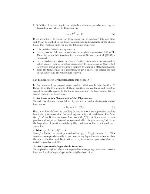
3. Definition of the metric g in the original coordinate system by inverting thediagonalization defined in Equation (5):g = U T · g ′ · U. (7)If the mapping F is linear, the three steps can be combined into one step,and F can be applied to the tensor components, independently of the chosenbasis. The resulting metric g has the following properties:• It is positive definite and symmetric.• Its eigenvector field corresponds to the original eigenvector field of T.Thus, the tensor field topology in the sense of Delmarcelle et al. [HD95] ispreserved.• Its eigenvalues are given by F (λ j ). Positive eigenvalues are mapped tovalues greater than a, negative eigenvalues to values smaller than a butlarger then zero.The zero tensor is mapped to a multiple of the unit matrix.• Since the transformation is invertible, we get a one-to-one correspondenceof the metric and the tensor field is given.3.2 Examples for Transformation Functions F :In this paragraph we suggest some explicit definitions for the function F .Except from the first example all these functions are nonlinear and thereforecannot be directly applied to the tensor components. The functions we discusscan be classified in two groups:1. Anti-symmetric Treatment of the EigenvaluesTo underline the motivation defined by (4), we can define the transformationfunction as:F (λ) = a + σf(λ). (8)Here, a = F (0) defines the unit length, and σ ≠ 0 is an appropriate scalingfactor that guarantees that the resulting metric is positive definite. The functionf : IR → IR is a monotone function with f(0) = 0. If we want to treatpositive and negative Eigenvalues symmetrically it is f(−λ) = −f(λ). Fromthe large class of functions satisfying this condition we have considered threeexamples:a. Identity: f = id , f(λ) = λSince f is linear, the metric g is defined by g ij = F (t ij ) = a + σ · t ij . Thisequation corresponds exactly to our motivating Equation (4), where σ playsthe role of the time variable t. With σ < a/λ max we can guarantee that themetric is positive definite.b. Anti-symmetric logarithmic function:To emphasize regions where the eigenvalues change sign one can choose afunction f with a larger slope in the neighborhood of zero.