Determination of grasscutter age - African Journals Online (AJOL)

More documents

Recommendations

Info

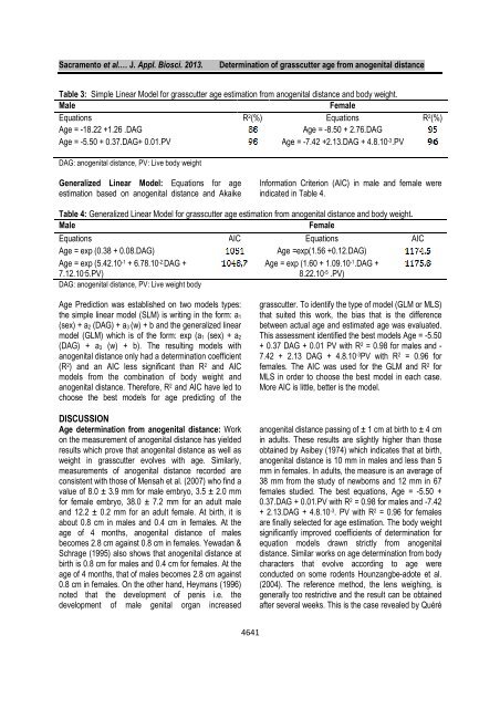
Sacramento et al.… J. Appl. Biosci. 2013.Determination of grasscutter age from anogenital distance• sheets for recording measured data.Manual restraint of grasscutter: Before anymeasurement, the animals were manually restrained.This manual restraint has been shown by Mensah &Ekué, (2003) and Mensah et al., (2007):• seize the animal almost at the base of the tail;• raise its hindquarters so that only the frontlegs are resting on the floor of the block• Then, slowly, carefully lift it completely fromthe ground making sure it does not turn on itself,because in this case the tail may dislocate and break.Once the animal content, it was introduced into theburlap bag and hung on the spring scale to gain weight.Measurement of anogenital distance: Themeasurement of anogenital distance involved allgrasscutters of all ages and sexes. For the success ofthis operation, three persons were used. In addition,disinfection of the caliper should be careful done toavoid transmission of diseases from one animal toanother. The measurement was made from smaller tolarger. Operations, which were repeated three times,took place as follows:• contention grasscutter supine;• installation of the caliper between the upperend of the anus and the lower end of the vulva;• Paired reading distance for accuracy.The measurements of a rodent’s anogenital distance,applied to grasscutters, were performed following themethod inspired by Rosevear (1969) and used bySicard et al. (1995). To perform these measurements,the grasscutter was lying on its back and its headfacing the left side. This allowed easy access tomeasurements on the same side and at different agesas follows: 2 weeks, 4 weeks, 8 weeks, 12 weeks, 16weeks, 20 weeks, 24 weeks, 28 weeks, 32 weeks, 36weeks, 40 weeks, 44 weeks and 48 weeks at afrequency of once a week. 5 to 10 min after anesthesia,grasscutters were removed from the cage and installedfor linear measurements and body weight.Method of anesthesia of the grasscutter: Once theweighing was completed, the grasscutter was taken outof the bag and then introduced into the restraining cagewhere it was anesthetized. Using 2 ml short syringes,RESULTSSimple Linear Model: Equations for age estimationbased on anogenital distance and coefficient ofsmall diameter and single-use needles, a mixture ofequal volumes of xylazine hydrochloride (Rompun 2%ND) and ketamine hydrochloride (Imalgene 1000 ND ) wasused in the same syringe at a dose of 0.1 ml / kg bodyweight. This method for anesthetizing grasscutter wasindicated by Adjanohoun (1986) and Farougou (1992)because the two products used separately are poorlytolerated by this rodent (Adjanohoun, 1988). On thebasis of animal body weight, the dose injected in eachanimal was calculated. This mixture injectedintramuscularly (IM) at the base of the tail, yielded agood sedation with excellent muscle relaxation at lowdoses. Anesthesia was effective after 5 to 10 minutesand the grasscutter slept for 30 to 60 minutes before itseffect wore off. This time was sufficient to take all linearmeasurements on the animal. All measurements weretaken early morning before feeding to avoid skewingthe data and frequency of once a week. Pregnantfemales were excluded from the study.Statistical analyses: The collected data were entered,coded and recorded using the Excel 2007 before beingprocessed. Descriptive statistics were performed. Thepairwise comparisons of means were performed usingStudent's test. The relationship between ages andvarious body measurements and weight weredetermined by calculating the correlation matrixbetween variables. This correlation provided guidanceon the simultaneous evolution of the variables taken inpairs. The coefficients of determination (R 2 ) for the MLSand the Akaike Information Criterion (AIC) for the MLGwere used to identify the best equation models. Forestablishing prediction equations, it was the simplelinear model (SLM) and the generalized linear model(GLM) that were used. In general, a predictive model isany equation that can be put in the form of: y = ax + b,with y the dependent variable, b the value of y when x =0; a change of y for any change in a unit of x, and x isthe independent variable. Once developed, thesemodels were used from independent samples. For dataprocessing we used the software R 2.10.0 with lots ofpackages (MASS, FactoMineR,).determination R 2 (%) in male and female were indicatedin Table 3.4640
Sacramento et al.… J. Appl. Biosci. 2013.Determination of grasscutter age from anogenital distanceTable 3: Simple Linear Model for grasscutter age estimation from anogenital distance and body weight.MaleFemaleEquations R 2 (%) Equations R 2 (%)Age = -18.22 +1.26 .DAGAge = -8.50 + 2.76.DAGAge = -5.50 + 0.37.DAG+ 0.01.PVAge = -7.42 +2.13.DAG + 4.8.10 -3 .PVDAG: anogenital distance, PV: Live body weightGeneralized Linear Model: Equations for ageestimation based on anogenital distance and AkaikeInformation Criterion (AIC) in male and female wereindicated in Table 4.Table 4: Generalized Linear Model for grasscutter age estimation from anogenital distance and body weight.MaleFemaleEquations AIC Equations AICAge = exp (0.38 + 0.08.DAG)Age =exp(1.56 +0.12.DAG)Age = exp (5.42.10 -1 + 6.78.10 -2. DAG +7.12.10 - 5.PV)Age = exp (1.60 + 1.09.10 -1 .DAG +8.22.10 -5 .PV)DAG: anogenital distance, PV: Live weight bodyAge Prediction was established on two models types:the simple linear model (SLM) is writing in the form: a 1(sex) + a 2 (DAG) + a 3 (w) + b and the generalized linearmodel (GLM) which is of the form: exp (a 1 (sex) + a 2(DAG) + a 3 (w) + b). The resulting models withanogenital distance only had a determination coefficient(R 2 ) and an AIC less significant than R 2 and AICmodels from the combination of body weight andanogenital distance. Therefore, R 2 and AIC have led tochoose the best models for age predicting of theDISCUSSIONAge determination from anogenital distance: Workon the measurement of anogenital distance has yieldedresults which prove that anogenital distance as well asweight in grasscutter evolves with age. Similarly,measurements of anogenital distance recorded areconsistent with those of Mensah et al. (2007) who find avalue of 8.0 ± 3.9 mm for male embryo, 3.5 ± 2.0 mmfor female embryo, 38.0 ± 7.2 mm for an adult maleand 12.2 ± 0.2 mm for an adult female. At birth, it isabout 0.8 cm in males and 0.4 cm in females. At theage of 4 months, anogenital distance of malesbecomes 2.8 cm against 0.8 cm in females. Yewadan &Schrage (1995) also shows that anogenital distance atbirth is 0.8 cm for males and 0.4 cm for females. At theage of 4 months, that of males becomes 2.8 cm against0.8 cm in females. On the other hand, Heymans (1996)noted that the development of penis i.e. thedevelopment of male genital organ increasedgrasscutter. To identify the type of model (GLM or MLS)that suited this work, the bias that is the differencebetween actual age and estimated age was evaluated.This assessment identified the best models Age = -5.50+ 0.37 DAG + 0.01 PV with R 2 = 0.98 for males and -7.42 + 2.13 DAG + 4.8.10 -3 PV with R 2 = 0.96 forfemales. The AIC was used for the GLM and R 2 forMLS in order to choose the best model in each case.More AIC is little, better is the model.anogenital distance passing of ± 1 cm at birth to ± 4 cmin adults. These results are slightly higher than thoseobtained by Asibey (1974) which indicates that at birth,anogenital distance is 10 mm in males and less than 5mm in females. In adults, the measure is an average of38 mm from the study of newborns and 12 mm in 67females studied. The best equations, Age = -5.50 +0.37.DAG + 0.01.PV with R 2 = 0.98 for males and -7.42+ 2.13.DAG + 4.8.10 -3 . PV with R 2 = 0.96 for femalesare finally selected for age estimation. The body weightsignificantly improved coefficients of determination forequation models drawn strictly from anogenitaldistance. Similar works on age determination from bodycharacters that evolve according to age wereconducted on some rodents Hounzangbe-adote et al.(2004). The reference method, the lens weighing, isgenerally too restrictive and the result can be obtainedafter several weeks. This is the case revealed by Quéré4641
Page 1 and 2: Sacramento et al.… J. Appl. Biosc
Page 3: Sacramento et al.… J. Appl. Biosc
Page 7: Sacramento et al.… J. Appl. Biosc

Determination of grasscutter age - African Journals Online (AJOL)

You also want an ePaper? Increase the reach of your titles

Delete template?

Save as template?