GMOS Data Reduction

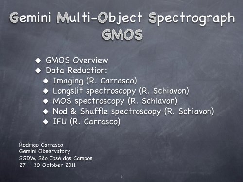
eminiulti- bject pectrograph GMOS Overview Data Reduction: Imaging (R. Carrasco) Longslit spectroscopy (R. Schiavon) MOS spectroscopy (R. Schiavon) Nod & Shuffle spectroscopy (R. Schiavon) IFU (R. Carrasco)Rodrigo CarrascoGemini ObservatorySGDW, São José dos Campos27 – 30 October 20111

Winter at Cerro Pachón

to the detectorMask assembly withcassettes and masksGrating turretFilter wheels7

OIWFS and patrol field areaIntegral Field UnitCassette # 1

GMOS Images: Data ReductionGeneral guidelines and suggestions" Fetch your program using the Observing Tool" Check the notes added by the observer(s) and/or the QueueCoordinator(s) regarding your observations" Check the observing log (you can use the OT)

GMOS Images: Data ReductionTypical GMOS imaging observations" Science Observations" A sequence of exposure using one or more filters." The sequence normally has offsets to avoid the gapsbetween CCDs." Daytime calibrations (Baseline) – GN(GS)-CALYYYYMMDD" Routine Bias for all binning (slow/fast readout, low gain)." Routine twilight flats for 2x2 binning (all filters)." Processed bias and twilight flats are in the GSA, but notover-scan subtracted" Nighttime calibrations (Baseline) - GN(GS)-CALYYYYMMDD" Photometric standard stars - zero point calibrations" Blank fields – fringe correction (i’ and z’ filter only)

GMOS Images: Data Reduction" Basic IRAF data reduction information in the web." Good starting point to reduce your" Dataset" SV data on Hickson Compact Group 87 from 2003" Observations with g, r and i filters, 1 x 1 (no binning)" Offsets between exposures to avoid gaps

GMOS Images: Data ReductionReduction Steps" Combine bias (trim, overscan)" Twilight flats : over-scan, bias subtraction, trim and combinethe frames" Science images: bias and over-scan subtraction, trim and flatfieldthe frames" Blank fields to construct a combined image for fringingcorrection (i-band only)" Mosaic the images and combine the frames by filter

Reducing GMOS Images" Be sure to use the correct bias slow readout/low gain,1x1 binning" GSA gives you a processed combined bias, but not over-scansubtracted. Check also for compatibility (binning, read mode)" Tip: check keyword AMPINTEG in the PHU" AMPINTEG = 5000 – Slow, AMPINTEG = 1000 – fast" Gain -- in the header, CCDSUM (ext)- binning" Bias reduction -- uses gbiasBias" Overscan subtr. – recommended" gbias @bias.list bias_out.fits fl_trim+ fl_over+ rawpath=dir$" Check the final combined bias image

Reducing GMOS ImagesTwilight flats" Twilight flats are used to flat field the images and removeartifacts caused by variations in the pixel-to-pixel sensitivity ofGMOS detectors" 20 to 25 flats per filter per month are observed duringtwilights under good weather, using a special dithering pattern." Final flat is constructed using giflat" giflat @flat_g.lst outflat=gflat bias=bias.fits fl_over+rawpath=dir$" The default parameters work ok for most cases" Over-scan is recommended" Final flat is normalized

" Removing the fringingReducing GMOS ImagesFringing correction" Significant fringing in i and z bands (worse with GMOS-S)" Blank fields for fringing removal observed every semesterin i and z (2x2 binning, slow readout/low gain)." Best fringing correction - use the same science images" Constructing the fringing frame with gifringe" using bias, over-scaned, trimmed and flat-fielded images." gifringe @fring.lst fringeframe.fits" girmfringe @inp.lst fringeframe.fits" Output = Input - s * F" s = stddev(Inp)/stddev(Out) for fl_statscale=yes" s = exptime(Inp)/exptime(Out) for fl_statscale = no (DEFAULT)

Reducing GMOS ImagesScience images" Reducing the images with gireduce" gireduce: gprerare, bias, overscan and flatfield the images" gireduce @obj.lst fl_bias+ fl_trim+ fl_flat+ fl_over+bias=bias.fits flat1=flatg flat2=flatr flat3=flati rawpath=dir$" Removing fringing with girmfringe (i band images only)" Inspect all images with gdisplay" Mosaicing the images with gmosaic - > gmosaic @redima.lst" Combining your images using imcoadd" imcoadd - search for objects in the images, derive a geometricaltrasformation (shift, rotation, scaling), register the objects in theimages to a common pixel position, apply the BPM, clean thecosmic ray events and combine the images

Final GMOS imageHCG 87

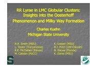
Integral-Field Spectroscopy Obtain a spectrum atevery position20

Integral Field SpectroscopyEach spectrum givesLagos et al. (2009)

IFU Zoo: How to map 3D on 2DGMOS“Spaxel”

GMOS IFU" Optical Integral Field Spectrograph" Lenslet-fiber based design" Various spectral capabilities" Two spatial setting" “Two slit” mode:- 5”x7” (5”x3.5” sky)- 3,000 spectral pixels- 1500 spectra (500 sky)" “One slit” mode:- 5”x3.5” (5”x1.75” sky)- 6000 spectral pixels- 750 spectra (250 sky)" Spatial sampling of ~0.2” per fiber" Dedicated sky fibers 60” offset for simultaneous sky

GMOS Example 2 slit mode M32

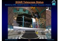
GMOS Example: 1 slit mode Mrk996SkyblocksObjectblocksChip gapsR slitWavelength

How is the 3D data mapped ?

GMOS IFU: Mask Definition Files" Mask Definition File (MDF) providessky coordinates of each fibre on CCDgnifu_slits_mdf.fits" Together with wavelength calibration,provide translation from CCD (X,Y) todata-cube (RA, DEC, λ)Slit mode GMOS-N GMOS-S2 Slit gnifu_slits_mdf.fits gsifu_slits_mdf.fits1 slit mode (Blue) gnifu_slitb_mdf.fits gsifu_slitb_mdf.fitsN & S 2 Slit modeN & S 1 slit mode (Blue)gnifu_slitr_mdf.fitsgsifu_slitr_mdf.fitsgsifu_ns_slits_mdf.fitsgsifu_ns_slitb_mdf.fitsgsifu_ns_ slitr_mdf.fits

GMOS IFU: Mask Definition FilesScience FieldSky Fieldgnifu_slits_mdf.fits" Mask Definition File (MDF) provides sky coordinates of eachfibre on CCD" Together with wavelength calibration, provide translation fromCCD (X,Y) to data-cube (RA, DEC, λ)

GMOS IFU ReductionOrganizing your files: suggestionRaw data:calibrations/ - all baseline daytime calibration raw imagesscience/ - all science datastandards/ - photometric standard stars (nighttime calibrations)Reductions:reductions/ - all reductionscalibrations/ - reductions of daytime calibrationsObj1/ - reduction of the first science objectGrating1/ - first gratingGrating2/ - second gratingcombined/ - combined imagesObj2/ - reduction of the second science objectfluxstandard/ - flux calibration

GMOS IFU ReductionTypical GMOS IFU observations" Science Observations" Acquisition" Direct image of the field initial offsets" Un-dispersed IFU image fine centering" Observation sequence:" Flat (fringing is flexure-dependent)" Science Exposure (up to 1 hour)" Flat (and CuAr arc if you need good Wavev. Calib.)" Daytime calibrations (Baseline)" Bias - GN(GS)-CALYYYYMMDD" Twilight sky flat and CuAr arcs (inside the program)" Nighttime calibrations (Baseline) - GN(GS)-CALYYYYMMDD" Flux standard for relative flux calibration (not – coincident)

GMOS IFU Reduction -> acquisitionGMOS GMOS IFU-2 IFU-2 reconstructed slitsGMOS direct (undispersed) imaging (undispersed)with image IFU-2 IFU-1 pseudo-slit1 arcminIFU RedIFU Blue

GMOS IFU ReductionTypical GMOS IFU raw dataScience Object Arc Flat LampBlockofskyfibersFiberWavelength

GMOS IFU Reduction" Basic IRAF data reduction information in the web." Good starting point to reduce your" Dataset" SV data on NGC 1068 from 2001" 2-slit mode IFU 5”x7” per pointing" 2x2 mosaic for field coverage" B600 grating, targeting H α and continuum" Bias is prepared already" Twilight sky included" Flux standard also included (not described here)

GMOS IFU ReductionStep to follow Bias and over-scan subtraction from all images (sciencespectra, flats, twilight sky, CuAr arcs, etc) – recommended Identify the fibers using a flat image Construct the FlatI. Spectral flat field to correct for transmission function using the GCAL flats

Step 1: bias subtraction" Use gprepare on your data (Science, flats, CuAr arcs). Thetask will add the MDF to the frames" Suggestion copy the MDF file to your local directoryin case that you need to edit it gnifu_slits_mdf.fitsgprepare @obj.lst rawpath=rawdir$ fl_addmdf+\mdffile=”gnifu_slits_mdf.fits” mdfdir=”gmos$data/”!" Use gfreduce for bias and over scan subtraction" Suggestion: do this interactivelygfreduce g//@obj.lst fl_addmdf- fl_inter+ \!fl_over+ fl_extract- fl_gsappwave- fl_wavtran- \fl_skysub- fl_fluxcal- fl_gscrrej- slits=both!

Step 2: identifying the fibers (spectra)" CRUCIAL step make sure the spectra can be traced on thedetector.Dead fiber" Use the flat lamp (high S/N) to find the fibers on thedetector, and trace them with wavelength" Once again, we use gfreduce interactively" We want to identify and trace the fibers only" There are dead fibers don’t want miss-identificationgfreduce rgN20010908S0105 fl_addmdf- fl_trim- \fl_bias- fl_wavtran- fl_skysub- fl_gscrrej- \fl_fluxcal- fl_inter+ slits=both!

Step 2: identifying the fibers (spectra)Fibers are in groups of 50 –inspect the gaps betweengroups

Step 2: identifying the fibers (spectra)Step 1: Where are the spectra?

Step 2: identifying the fibers (spectra)Trace of one fiberJump to CCD2Contaminationfrom slit_2?

Step 2: identifying the fibers (spectra)Trace of one fiberJump to CCD2Contaminationfrom slit_2?

Step 2: identifying the fibers (spectra)Non-linearcomponentRejectedpoints

Step 2: identifying the fibers (spectra)Jump to CCD2

Step 2: identifying the fibers (spectra)" Following extraction, data are stored as 2D images in oneMEF (one image per slit) ergN20010908S0105" This format is VERY useful for inspecting the datacube~750FibersWavelength

Step 3: prepare the flat-field" Flat-fielding has two components:" Spectral Flat-field Correct for instrument spectral transmission response Use black body lamp and divide by fitted smooth function" Spatial Flat-field: Correct for illumination function & fiber response Use Twilight sky flat to renormalize the (fit-removed) flatlamp" But first, we have to trace the fibers for twilight sky flat usingthe processed flat image as reference to trace the fibers gfreduce looks in the “database/”gfreduce rgN20010908S0112 fl_bias- fl_over- fl_gscrrej- \fl_wavtran- fl_skysub- fl_inter+ slits=both tracerecenter+ref="ergN20010908S0105”!

Step 3: prepare the flat-field" Make response curves with twilight correctiongfresponse ergN20010908S0105 ergN20010908S0105_resp112sky=ergN20010908S0112 order=95 fl_inter+ func=spline3sample="*"!Likely start offringingeffectsFinalflat

Step 4: wavelength calibrationHow can we re-sample the data to have linear wavelength axis? Find dispersion function: relationship between your pixels andabsolute wavelengthWavelengthCCD pixels

Step 4: wavelength calibration" Note that the arc in the tutorial has not been observed in thescience sequence." CuAr arcs – over-subtract instead of using the bias since thebias does not apply to fast read and low gain" Using the flat to trace the fibers.gfreduce N20010908S0108.fits fl_wavtran- fl_inter+ref=ergN20010908S0105 recenter- trace- fl_skysubfl_gscrrej-fl_bias- fl_over+ order=1 weights=nonebiasrows!" Establishing wavelenght calibrtationgswavelength ergN20010908S0108 fl_inter+ nlost=10!

Step 4: wavelength calibrationFirst step: Identify lines in your arc frameReference list for thislamp from GMOS webpage

Step 4: wavelength calibration" Marked lines in GMOS spectrum, after some tweaking…

Step 4: wavelength calibrationNon-linearcomponent of fit

Step 4: wavelength calibrationRMS ~0.1 pix" First solution used asstarting point forsubsequent fibers" Usually robust, butshould be checkedcarefully." Often best to edit thereference line file(CuAr_GMOS.dat)." Two slits are treatedseparately – need torepeat

Step 4: wavelength calibrationChecking the wavelength calibration" Testing quality of wavelength calibration is critical" Not always obvious from your science data" May not have skylines." Detect nonlinearity systematics" Basic check is to apply the calibration solution to the arcitself, and inspect the 2D imageSlit 1~1500FibersSlit 2Wavelength

Step 4: wavelength calibrationChecking the wavelength calibration" Twilight sky is also an excellent test" Reduce it like your science data" Check alignment of absorption dataSlit 1" Can also be compared with the solar specrum" Correlae with solar spectrum to get “velocity field” oftwilight.Slit 2" Can be sensitive to other effects, like fringing Slit 1~1500FibersSlit 2Wavelength

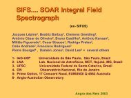
The effect of fringing from bad flatMcDermid et al. 20067060150100SINFONI dataon NGC 4486ay (px)5040302010500v (km/s)-50-100Nowak et al.10 20 30 40 50 60x (px)-150Such effects would be completely missed in long-slit data….

Step 5: reducing the science data" Now run “gfreduce” on science data to (bias subtractionalready done): Extract traces using the flat as a reference Apply flat-fielding correction (output from “gfresponse”) Cleaning cosmic rays using a Laplacia filter LaplacianCosmic Ray Identification routine by P. van Dokkum Apply wavelength solution and rectify the spectra Sky subtractiongfreduce rgN20010908S0101 slits=both fl_inter- fl_overfl_bias-fl_wavtran+ fl_flux- refer=ergN20010908S0105recenter- trace- wavtran=ergN20010908S0108response=ergN20010908S0105_resp112 slits=both

Step 6: Constructing Data CubeData cube is constructed with “gfcube” Resample extractedIFU spectra onto an x-y- datacubegfcube stergN20010908S0101 sample=0.1 fl_atmdisp+" sample=0.1 spatial sampling rate or pixel size to use in theoutput datacube." fl_atmdisp=yes Compensate for atmospheric dispersion(differential refraction) when resampling the fibre spectra ontothe output datacube" Differential atmospheric refraction (DAR) estimated using theatmospheric model from the version of SLALIB distributedwith IRAF (v2.3.0 as of gemini v1.10) “help refro”

Differential Atmospheric Refraction" Lack of atmospheric dispersion compensator (ADC) in bothGMOSs" Atmospheric refraction = image shifts as function of wavelength" Shift larges at blue wavelength0.5”" Can be corrected during reduction by shifting back each λplane or …" Use “gfcube” (fl_atmdis=yes). The correction is relatively good.OR…" Can use the approach given by Arrivas et al. (1999) for DAR IFUcorrection." http://www.gemini.edu/sciops/instruments/gmos/itcsensitivity-and-overheads/atmospheric-differential-refraction