Math 150 Study Guide

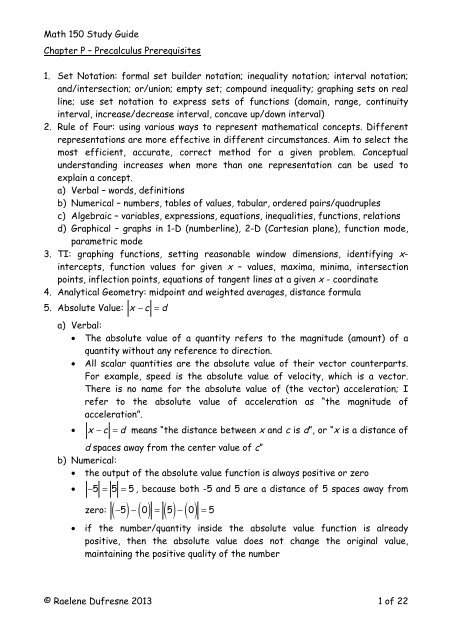
Math 150 Study Guide24. Extrema and Intervals Increasing/Decreasinga) Increasing on an interval is a positive change in x yields a positive change in y.b) Decreasing on an interval is a positive change in x yields a negative change in y.c) Constant on an interval is a positive change in x yields no change in y.d) monotone = alwayse) Interval of increase (or decrease): the set of x values for which the functionis increasing (or decreasing).f) Local maximum: a y value that is greater than or equal to all other y values oneither side of that point.g) Absolute maximum (also a local maximum): the largest y value in the entirerange of the functionh) Local minimum: a y value that is less than or equal to all other y values oneither side of that point.i) Absolute minimum (also a local minimum): the smallest y value in the entirerange of the function25. Concavity and Points of Inflectiona) A measure of the curvature of a relation.b) Upwards concavity at a point is visible when a tangent (line) to the curve at apoint lies below the curve (except at the point of tangency).c) Downwards concavity at a point is visible when a tangent to the curve at a pointlies above the curve (except at the point of tangency).d) A point where the concavity changes is a point of inflection.26. Boundednessa) Bounded below: there is some number (height of graph) that is less than orequal to all other y – coordinates.b) Bounded above: there is some number (height of graph) that is greater than orequal to all other y – coordinates.c) Bounded: bounded above and belowd) Unbounded: bounded neither above nor below27. Symmetrya) Even• Reflective symmetry about the y – axis• Horizontal reflection produces the original graph• f −x( ) = f ( x )b) Odd• Rotational symmetry about the origin• Horizontal reflection is equivalent to the vertical reflection• f −x( ) = −f ( x )© Raelene Dufresne 2013 7 of 22

y = −x 2 or − y = x 2Math 150 Study Guideoperations: multiply first (so do reflections and then scales), and then add (dotranslations y = x 2 y last).= e xy = e −x33. Five Kinds of Reflections( ) is a vertical reflection of the graph of( ) through the x – axis (or line y = 0 ).a) Vertical Reflection (VR): y = −f xy = f xb) Partial Vertical Reflection (PVR): y = f x( ) is a partial vertical reflection( ) that has( ) arethrough the x – axis, for the part(s) of the graph of y = f xnegative y – coordinates. The y – coordinates of the graph of y = f xnon-negative.y = x 2 − 3 y = x 2 − 3 y = − x 2 − 3c) Horizontal Reflection (HR):© Raelene Dufresne 2013 10 of 22

Math 150 Study Guidene) Division algorithm: f ( x )( x )=d ( x ) = q ( x ) +f) Improper Form:• degree of numerator greater than or equal to the degree of the numerator• use in factored and reduced function form to find coordinates of any holes,x – intercepts and equations of VAg) Proper Form:• degree of numerator less than the degree of the numerator• y = q x( )( )r xd x( ) is the non-vertical asymptote( ) are x – coordinates where f ( x ) I q ( x )( ) are the equations of the VAsr ( x )d ( x )• real zeroes of r x• real zeroes of d x• Consider thatacts as a "variable vertical translation” on the morerbasic graph of y = q ( x ) to get the rational function graph, y = q ( x )( x )+d ( x )h) Transformational Form: some rational function equations can be rearrangedfrom the proper fraction form to look like a transformation of one of the twobasic rational functions, y = 1 x or y = 1 . You are not expected to be able to2xexpress all rational function equations in transformational form.i) Holes• Basic Hole: y = x x = ⎧⎪⎨1 if x ≠ 0, and by plotting a hole in the⎩⎪ not defined if x = 0graph of y = 1 at (or removing the point) ( 0,1), we get the graph of y = x x .• Removable discontinuity• Finite (or “defined”) x values that make y indeterminate• Occur whenever n x• If f ( m) = 0 0( ) and d ( x ) have a common factor that has real roots( ) = n (the limit exists and is equal to n), then f ( x )but lim f xx →m( ) .has a hole at m,nj) Vertical Asymptotes• Basic vertical asymptote of multiplicity one: The Reciprocal Function y = 1 x© Raelene Dufresne 2013 15 of 22

Math 150 Study Guide• Basic vertical asymptote of multiplicity two: The Reciprocal SquareFunction y = 1x 2• Infinite discontinuity• May NOT be touched or crossed• Finite (or “defined”) x values that make y undefined• Occur whenever the denominator has real roots• If lim f xx →m( ) = ∞ or - ∞ or ± ∞ (check the sign chart for one-sided and two-( ) has a vertical asymptote at x = m .sided limits), then f x• VA multiplicity of 1 or 2; multiplicity affects the sign chartk) Jump Discontinuity• Basic Jump: y = x x = x ⎧⎪−1 if x < 0= ⎨x ⎩⎪ 1 if x > 0• Occurs when an x –value makes y indeterminate AND the function involvesan absolute valuel) End Behaviour/Non-Vertical Asymptotes• Zoomed out behaviour, what the graph looks like when you zoom out farenough• May or may not be touched or crossed• Found as the quotient of a rational function ( y = q x( ) from the properfraction form); the degree of the quotient polynomial prescribes the “type”of non-VA: horizontal, slant, parabolic, etc.. Furthermore, the type dependsof the difference in the degrees of the numerator and denominatorpolynomialsm) Special Case of Non-VA: Horizontal (constant quotient) Asymptote• Non-VA of degree 0• Infinite x produces finite y (compare with vertical asymptotes, for whichfinite x produces infinite y)( ) = k means that y = k is a horizontal asymptote of f ( x )• lim f xx →±∞n) About the different equation forms: Recognize various forms for equations ofrational function graphs, be able to extract properties from various equationforms, be able to graph from such forms, be able to determine the mostappropriate form in given situations, and be able to rearrange from one formto another42. Solving Equations in One Variable:a) get LCD© Raelene Dufresne 2013 16 of 22

Math 150 Study Guideb) consider domain restrictions to eliminate possible extraneous solutionsc) clear fractions by multiplying both sides of the equation by the LCDd) solve the resulting polynomial using factoring, rational root theorem, etc.e) eliminate any extraneous solutions43. Solving Inequalities in One Variable:a) never solve as an equation! (Well, there are a few instances when you can, butin general, and usually, you cannot.)b) solve graphically by comparing heights of two different functions (the leftside and right side functions)c) be clever in rearranging terms in the inequality to make solving by graphingeasier. For example, rearrange x 2 + 2x + 5 > 0 as x 2 + 2x > −5 , both of whichare easy to sketch; you should quickly note that y = x 2 + 2x is ALWAYShigher than y = −5 and therefore the solution is x ∈° .d) Solve by sign chart (which is a numerical and partial graphical method), usefulwhen the complete graph is not required. VERY IMPORTANT NOTES:• All terms must be on one side (let’s say the left) and ZERO on the other• The expression on the left must be FULLY FACTORED; all factors(expressions in parentheses) then must be joined either by multiplication ordivision, NOT by addition and subtraction. (Why? Do you know what (-)times (-) is? YES .. positive. But do you know what (-) + (-) is? No ... itdepends on HOW BIG each negative quantity is.44. Graph: Know all steps and required informationa) absolute value, polynomial, power/root, greatest integer, rational, exponential,logarithmic, logistic and piecewise functions and some relations (circles andhorizontal parabolas) by handb) use sign charts to aid in graphing functions45. Modeling and Optimization:a) Regression curves; scatter plots; interpolation and extrapolationb) Real world domain restrictions and extraneous solutionsc) Writing word problems algebraicallyd) Geometry formulas• Circle: C = 2πr and A = πr 2• Surface Area: sum of all surfaces’ areas• Volume: V = 1 n A ⋅ h , where n = 1,2 or 3basee) Optimization (max/min word problems)• Define all quantities using meaningful variables different from x and y• Define independent quantities using lower case variables and dependentquantities using upper case variables© Raelene Dufresne 2013 17 of 22

Math 150 Study Guide• Write equations for all dependent variables in terms of the independentvariables; use function notation.• Identify the dependent quantity to be optimized (of which you want themaximum or minimum).• Identify any information that relates the independent variables and writeequations from that information. You’ll recognise this because a value forthe dependent quantity (like volume of 1000 cm 3 ) will be given. Use thisequation to make a substitution for one independent variable in terms ofthe other. Be clever in your choice ... keep the independent variable thatyou wish to solve for (if you only need to solve for one independentvariable), or eliminate the variable that is algebraically simpler if you needto solve for both independent variable.• Once you have expressed the dependent quantity to be optimized in termsof the single independent variable, rename the variables x and y.• State the domain of the real world problem. Extrema can occur atendpoints, so you need to check the y values of any closed interval domains.f) Physics• 1-dimensional motion of a particle: motion is a synonym for velocity (whichmay be constant or change) of an object in one dimension (either vertically,up and down, or horizontally, right and left, but not the “projectile motion”where the object moves horizontally and vertically, concurrently. Projectilemotion is 2-D motion). The relevant quantities to be analysed include: time,position (i.e., height is vertical position), velocity, speed, acceleration.• free-fall: constant acceleration due to the force of gravity, thereforelinear velocity and quadratic height functions, and the (same) time-domainof these functions• speed is the absolute value (PVR) of velocity• writing the position, velocity, speed and acceleration functions of timegiven initial position, initial velocity and constant acceleration• dimensional analysis (verification by units)• ordered quadruplesChapter 3 – Exponential, Logistic and Logarithmic Functions47. Properties of logarithms48. Population Modeling49. Equivalent functions, domain restrictions, (true or false and explain), usingalgebraic identities and graphing50. Transformations51. Finances: simple/compound interest and continuously compounded formulas52. Richter Scale53. pH54. Newton’s Law of Cooling55. Exponential Growth and Decay© Raelene Dufresne 2013 18 of 22

Math 150 Study GuideChapter 4 – Trigonometric Functions81. Degree-radian conversion82. Standard position of angles83. Trig tools: two special triangles, the CAST “Rule”, the Unit Circle84. Pythagorean Triples (which do NOT have anything to do with the 30, 45, 60degree angles of the two special triangles)85. Domain restriction: hypotenuse must be the largest side of a triangle86. inverse trig function is NOT a reciprocal trig function87. Angles: acute, principal, coterminal, negative88. Reference triangles (reflected from QI into the other three quadrants)89. Basic trig function graphs and their transformations90. Connecting HS to period to number of cycles in a 2π interval for trig functions91. Writing coterminal angle formulas92. Evaluating trig and inverse trig functions for acceptable (domain) values93. Domain and Range for trig and inverse trig functions94. angles are inputs of trig functions; ratios are outputs; vice versa for inverse trigfunctions95. Solving trig functionsa) graphicallyb) algebraicallyc) by hand and with TI (use of domain restrictions, “such that”)96. Solving word problems involving acute triangles97. Sinusoidal modeling:a) ferris wheel height versus timeb) rabbit population versusc) tide height versus time98. Angular and linear distance: s = θr (circumference is a special case)99. Angular and linear speed: v = ωr100. Area of a sector of a circle (includes area of a complete circle)101. Sketching a point on a terminal arm in standard position, and stating all trigratios for the resulting angle102. getting reference angles: example 53π103. trig θ104. trig θ7( ) = trig( θ coterminal )( ) = ±trig( θ reference ) , depending on the quadrant (if a nonquandrantal angle)⎛ x ⎞105. Write an algebraic expression for expressions like sin⎜cos −1 ⎟ and stating⎝ x + 2⎠domain restrictions106. OMIT: Simple Harmonic Motion – we did not cover this© Raelene Dufresne 2013 20 of 22

Math 150 Study GuideChapter 5 – Analytical Trigonometry107. Know all fundamental trig identitiesa) Reciprocalb) Quotientc) Pythagoreand) negative anglee) cofunctionf) sum/differenceg) double angleh) power reducing/half anglei) Apply fundamental trig identities to evaluate trig ratios of non-special angles( 22.5o , 75o , 165 o )108. Apply fundamental trig identities to evaluate trig ratios of non-special angles⎛ 1expressed in terms of inverse trig functions: tan cos −1 3 − 4⎞⎜ sin−1 ⎟⎝5⎠109. Apply fundamental trig identities to simplify more complicated trigexpressions in order to:a) prove an identityb) sketch a basic transformed sinusoid in disguise/identify period & amplitudec) solve trig equations110. Solve trig equations:a) using factoring (never divide by an expression that may equal zero!)b) using trig identities to simplify firstc) determine reference angles and quadrants (where necessary)d) solve for all principal anglesa. solve for all coterminal angles to the principal solutionsb. solve a trig equation on the HOME screen and interpret @n1 (etc)c. solve graphically for x - intercepts or intersection points111. Recognize whether two seemingly equivalent functions (trig or other type)have the same domain or not: TRUE or FALSE and EXPLAIN!!!112. Create a geometric proof using lines and circles involving angles113. Understand the difference between an always true, a sometimes true, and anever true statement114. DO NOT distribute non-linear functions:a. know that sec 75 o( ) = sec ( 30 o + 45 ) o ≠ sec30 o + sec 45 o1b. know that sec 75 o =cos 75 = 1ocos 30 o + 45 o( )1=cos30 o cos 45 0 − sin30 o sin 45 o© Raelene Dufresne 2013 21 of 22

Math 150 Study Guide≠1cos30 o cos 45 − 10 sin30 o sin 45 0= sec30 o sec 45 o − csc30 o csc 45 o and explain why not!Chapter 6115. Vectorsa) rectangular componentsb) polar componentsc) P -> R and R -> P conversion by hand and on the TId) Unit vector notation (uses rectangular components)e) Adding vectors (must be done using rectangular components)116. Complex Numbersa) standard form (like rectangular components of a vector)b) trigonometric form (like pole components of a vector)c) Euler’s Formula: e iθ = cosθ + i sinθ = cisθd) multiplying two complex numbers (shortcut)e) dividing two complex numbers (shortcut)117. Vector valued functions: determine the magnitude (r) and direction (θ ) for arvector function at a specific time: v tĵ . Example: for( ) = ( 14t ) î + ( −5t 2 + 10t + 2) rv ta) The rectangular components : v 1b) The polar components are:ĵ , at time t = 1 ,( ) = 14î( ) = x ( t ) î + y ( t )− 7ĵ = ⎡14, −7⎤⎣ ⎦( ) 2 = 7 5 and θ IV= 360 o − tan −1 1r = 14 2 + −72 333.435o118. There is NO PROJECTILE MOTION in parametric mode on the exam.© Raelene Dufresne 2013 22 of 22