Effect of Hub Motor Mass on Stability and Comfort ... - Protean Electric

<strong>Effect</strong> <strong>of</strong> <strong>Hub</strong> <strong>Motor</strong> <strong>Mass</strong> on Stability and Comfort <strong>of</strong>
Electric Vehicles
D.J. van Schalkwyk and M.J. Kamper
Electrical Machines Laboratory, Department <strong>of</strong> Electrical and Electronic Engineering, University <strong>of</strong> Stellenbosch
Stellenbosch, South Africa 7602, Email: kamper@sun.ac.za
Abstract – <strong>Hub</strong> motors have always been considered as
propulsion for electric vehicles, but not widely used due to
various negative aspects. One <strong>of</strong> these is the uncertainty <strong>of</strong> the
effect the added wheel mass has on the stability, safety and
comfort <strong>of</strong> the vehicle. In this paper, frequency analysis as well as
simulations <strong>of</strong> the system is done using a simple model that
represents the vehicle suspension system and wheels. The results
<strong>of</strong> the hub driven vehicle are compared to that <strong>of</strong> a standard
vehicle. It is shown that the added wheel mass has no effect on
the stability <strong>of</strong> the vehicle and that the frequency response is
within the accepted comfort range.
Index Terms – hub motor; natural frequency; suspension system;
I. INTRODUCTION
With the introduction <strong>of</strong> hub motors to the world <strong>of</strong>
electric vehicles, a critical question has arisen: ‘What effect
has the added wheel mass <strong>of</strong> a hub motor on the safety and
comfort <strong>of</strong> a vehicle?’ Moving the propulsion from the vehicle
body to the wheels can add up to 50 kg or more, per wheel, to
the unsprung mass. Most <strong>of</strong> the research done on suspension
systems has been done for standard vehicles [1]. No real
investigations have been done on increased unsprung mass. A
few recommendations state that the unsprung mass should not
exceed 20% <strong>of</strong> the sprung mass [2]. Current road vehicles do
not exceed this ratio and no real evidence supports this ratio.
By increasing the mass <strong>of</strong> the wheel, the wheel inertia is
increased. Increased wheel inertia causes higher acceleration
forces during road condition reaction. These forces put
relatively high levels <strong>of</strong> stress on contact and connection
points <strong>of</strong> the wheels. These forces can also cause degradation
in ride comfort as experienced by the occupants <strong>of</strong> the vehicle.
The aim <strong>of</strong> the investigation is to study, through frequency
analysis and simulation, the effect <strong>of</strong> moving mass from the
sprung mass to the unsprung mass <strong>of</strong> a vehicle. The
simulation results are compared with that <strong>of</strong> a standard vehicle
to ascertain if it is possible to increase the unsprung mass <strong>of</strong> a
vehicle.
The added mass has an effect on the handling <strong>of</strong> the vehicle as
well. It is beyond the scope <strong>of</strong> the study to investigate this
area, as the models and analyses are complex. These will be
investigated in a later study to verify the first results as well as
simulate vehicle handling. It is the opinion <strong>of</strong> the author that
this study will give enough information to make sufficient
conclusions on the effect <strong>of</strong> increased unsprung mass.
II. VEHICLE MODEL
A. Quarter Vehicle Suspension Model
The vehicle is modeled using a two-degree-<strong>of</strong>-freedom
(2DOF) system [3]. The system comprises <strong>of</strong> two masses
suspended by two sets <strong>of</strong> spring-damper systems. The
advantage <strong>of</strong> using a 2DOF system is that it gives a simple yet
accurate model <strong>of</strong> the vehicle’s mass-suspension system and
tire. The model allows observation <strong>of</strong> both suspension and tire
deflection under applied road conditions. This model is a
standard model used in suspension simulations [1, 4]. It
represents a quarter <strong>of</strong> the vehicle and is thus called a quarter
vehicle suspension model.
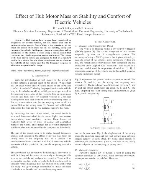
Fig. 1 represents the quarter vehicle suspension model. The
masses, Mv and Ms, are the sprung and unsprung mass
respectively. The two damper coefficients are given by Bs and
Bt and the spring coefficients are given by Ks and Kt. The
road, unsprung mass and sprung mass displacement is given
by x, y and z respectively.
Mv
Bs Ks
Ms
Bt Kt
Fig. 1 Quarter vehicle suspension model.
As can be seen from Fig. 1, the displacement <strong>of</strong> the sprung
mass, the unsprung mass and the road surface have different
origins relative to each other. By using these frames <strong>of</strong>
reference, the displacements, y and z, can refer to any solidly
connected point on the unsprung or sprung mass.
B. Dynamic Equations
Newton’s second law <strong>of</strong> motion is used to derive the
dynamic equations <strong>of</strong> the system. Since there are two bodies,
two equations need to be satisfied. These are:
M z
(1)
V
= FV
M z
(2)
S
= FS
z
y
x

The two forces Fv and Fs, which are the forces acting on the
sprung and unsprung mass respectively can be found through
inspection <strong>of</strong> Fig. 1. The dynamic equations <strong>of</strong> the system
become:
= −K
S ( z − y)
− BS
( z − y)
− M g
(3)
= K ( z − y)
+ B ( z − y)
− K ( y − x)
− B ( y − x)
− M g (4)
MV z
V
M S y S
S
T
T
S
C. Wheel Hop
A very real phenomenon is that <strong>of</strong> the tire losing contact
with the road surface, also known as “wheel hop”. This
phenomenon needs to be taken into account as it could happen
during the simulations that the tire looses contact with the
road due to either fast changing road conditions or the
instability <strong>of</strong> the suspension system.
The last point <strong>of</strong> contact between the tire and the road surface
occurs when the unsprung mass and the road surface is
equally displaced from their respective origins i.e. y-x=0. The
force due to the tire spring and damper are only exerted when
the wheel is in contact with the road surface. Incorporating
wheel hop into the dynamic equations, (4) becomes:
= K S ( z − y)
+ BS
( z − y)
− KT
( y − x)
− BS
( y − x)
− M g (5)
if ( y − x)
≤ 0
= K S ( z − y)
+ BS
( z − y)
− M g
(6)
if ( y − x)
≥ 0
M S y
S
M S y
S
The wheel hop phenomenon adds a non-linearity to the
system. It has been decided that it can be neglected during the
frequency analysis <strong>of</strong> the system, but not for the simulations.
It will have little or no effect on the frequency response <strong>of</strong> the
system. It adds complexity to the analysis with little increase
in the accuracy <strong>of</strong> the results.
D. Vehicle Parameters
Two vehicles are compared in the study. One is a
standard vehicle and the other a vehicle with a hub motor
place in the rear wheels. The same total mass i.e. sprung and
unsprung mass combined, is used for both vehicles. A total
mass <strong>of</strong> 1500 kg was chosen. This is the mass <strong>of</strong> a fully laden
vehicle (vehicle mass, passengers and payload). All constants
used, such as damping and spring coefficients, are kept the
same for both vehicles. Table I gives a list <strong>of</strong> all the constants
used.
TABLE I
VEHICLE PARAMETERS
Standard Vehicle <strong>Hub</strong> Driven Vehicle
Total Model Total Model
Total <strong>Mass</strong> (kg) 1500 375 1500 375
Sprung mass (kg) 1340 335 1100 275
Unsprung mass (kg) 160 40 400 100
Ks (N/m) 36 000 36 000 36 000 36 000
Bs (Ns/m) 3000 3000 3000 3000
Kt (N/m) 110 000 110 000 110 000 110 000
Bt (Ns/m) 200 200 200 200
The standard vehicle will serve as the control for the
investigation and the hub driven vehicle as the experiment. As
the simulation uses the quarter vehicle suspension model, all
masses are a quarter <strong>of</strong> the real values.
III. FREQUENCY ANALYSIS
A. Bode-plot Analysis
It is important to verify that the suspension system and
the vehicle are, through system frequency response analysis,
stabile under changing road surface conditions. The simplest
method to investigate the frequency response <strong>of</strong> the system is
through a Bode-plot analysis. This can easily be done with the
help <strong>of</strong> s<strong>of</strong>tware like MatLab.
The transfer function is required to obtain the Bode-plot <strong>of</strong> the
system. The transfer function can be mathematically derived
from the dynamic equations or extracted from the linear model
using MatLab. From MatLab the transfer function for the
standard vehicle system is given as
( s)
G ST
3
2
8.
527e
−14s
+ 4.
093e
−12s
+ 2.
463e4s
+ 2.
955e5
= (7)
4
3 2
s + 88.
96s
+ 3802s
+ 2.
516e4s
+ 2.
955e5
and the hub driven vehicle system as
( s)
G HD
3
6.
395e
−14s
+ 3.
638e
−12s
+ 1.
2e4s
+ 1.
44e5
= (8)
4
3 2
s + 42.
91s
+ 1613s
+ 1.
226e4s
+ 1.
44e5
The transfer function can give an indication on the stability <strong>of</strong>
the system. Both transfer functions have higher order poles
than zeros. It can be seen that the second and third order zeros
are small in comparison with the rest. These are good
indicators that a system is stable. The Bode-plot will give an
even better indication on the stability <strong>of</strong> the system.
Fig. 2 Bode-plot <strong>of</strong> standard and hub driven vehicle.
2

A system is said to be unstable if it has a phase <strong>of</strong> -180
degrees at its crossover frequency. A system could also
possibly be unstable if the magnitude is larger than 1 dB when
the phase is equal to -180 degrees. From Fig. 2 and Table II it
can be seen that the standard and hub driven vehicle do not
meet these two criteria and thus are stable.
The dominant natural frequency <strong>of</strong> the system can easily be
seen from the Bode-plot. This natural frequency is where the
Bode-plot reaches a maximum. As both systems are 2DOF
systems, two natural frequencies occur. The first or lower
frequency will be the dominant natural frequency, with the
higher second frequency being the damped natural frequency.
The damped natural frequency is difficult to distinguish, but
can be found by looking at the shape <strong>of</strong> the Bode-plot. The
natural frequency can be calculated more accurately.
TABLE II
BODE-PLOT INFORMATION
Standard <strong>Hub</strong> Driven
First Natural Frequency (rad/s) 9 10
Second Natural Frequency (rad/s) 60 40
Crossover Frequency (rad/s) 15 18
-180 deg Frequency (rad/s) 52 33
Mag. at natural frequency (dB) 7 7.5
Something to note is that the two natural frequencies move
closer together as the mass is shifted from the body to the
wheels. When the natural frequencies are far apart the second
is extremely damped and plays virtually no part in the
oscillation <strong>of</strong> the system. As the two moves closer together,
the second frequency starts playing a larger role. The two
frequencies could move so close together, super positioning
on each other, causing larger and unwanted oscillations.
B. Natural Frequency Analysis
The natural frequency <strong>of</strong> a system is the frequency at
which a driving force causes maximum oscillation amplitude
or even unbounded oscillation. In multiple-degree-<strong>of</strong>-freedom
systems, the system has n number <strong>of</strong> natural frequencies. It is
possible that the system resonates at all, some or none <strong>of</strong> its
natural frequencies.
The natural frequencies <strong>of</strong> a 2DOF system are given as the
square-root <strong>of</strong> its eigenvalues, that is
ω
n
= λ
n
(9)
The eigenvalues <strong>of</strong> the systems are derived from the state
space equations. The eigenvalues are given as:
1 K S + KT
K S K S + KT
K S K S KT
λ =
+ −
+ − 4 (10)
1
2 M M M M M M
λ2
=
1
2
K
S
S
+ K
M
S
T
V
K
+
M
S
V
+
K
S
S
+ K
M
S
T
V
K
+
M
S
V
2
2
S
K S K
− 4
M M
S
V
T
V
(11)
The natural frequencies are calculated to be:
Standard vehicle: ω = 80.
368 = 8.
96 rad/s or1. 43 Hz
1
ω = 3677.
09 = 60.
639 rad/s or 9. 65 Hz
2
<strong>Hub</strong> driven vehicle: ω = 96.
349 = 9.
82 rad/s or1. 56 Hz
1
ω2 = 1494.
56 = 38.
659 rad/s or 6. 15 Hz
The calculated frequencies compare well with those given by
the Bode-plot. The inaccuracy <strong>of</strong> the Bode-plot figures is due
to the fact that the natural frequencies were obtained by
inspection.
The human body is sensitive to certain frequency ranges [4].
The vehicle will be classified as uncomfortable if the first
natural frequency falls within these ranges. It has been found
that frequencies between 0.5 and 1 Hz cause a high
occurrence <strong>of</strong> motion sickness. The human head and neck is
especially sensitive to vibrations between 18 and 20 Hz. The
abdomen region <strong>of</strong> the body is sensitive to vibrations between
5 and 7 Hz. Research has shown that a system with a natural
frequency higher than 3 Hz is perceived as a “harsh ride”. A
ride is deemed to be comfortable near the 1.5 Hz mark.
Taking the above mentioned frequency regions into account; it
is safe to stipulate a guideline stating that a comfortable
system would have a dominant frequency between 1 and 3 Hz.
It can be seen that the calculated frequencies fall within this
ranges. Furthermore they are close to 1.5 Hz which is
perceived as the optimum natural frequency.
C. Payload Analysis
The analysis in the previous section was done on the
suspension system <strong>of</strong> a fully loaded standard and hub driven
vehicle. The next step is to investigate the effect <strong>of</strong> varying
the payload on the natural frequency <strong>of</strong> the system. The
payload range from empty to fully load. A vehicle’s curb
weight is defined as the weight <strong>of</strong> the vehicle when it is fully
operational plus one passenger. An electric vehicle’s curb
weight is generally less than that <strong>of</strong> a standard vehicle, as is
the case in this section. The curb weights for a standard and
hub driven vehicle is chosen as 900 kg and 750 kg
respectively. Fig. 3 shows the dominant natural frequency for
both the standard and hub driven vehicles for a range <strong>of</strong>
payloads. The natural frequencies are calculated by means <strong>of</strong>
the equations used in the previous section.
It can be seen that the varying payload has little effect on the
natural frequency <strong>of</strong> the standard vehicle. On the other hand,
the natural frequency <strong>of</strong> the hub driven vehicle shows
significant variations due to the changing payload. This means
that the hub driven vehicle will have a more varying ride
response due to payload changes than the standard vehicle.
However, both the vehicle’s natural frequencies stay within
the 1 to 3 Hz range, although the hub driven vehicle’s
frequency nears the 3 Hz limit when empty.

Frequency (Hz)
2.8
2.6
2.4
2.2
2
1.8
1.6
1.4
1.2
1
0 100 200 300 400 500 600 700
Standard
<strong>Hub</strong>-driven
Payload (kg)
Fig. 3 Dominant natural frequency <strong>of</strong> standard and hub driven vehicles.
VI. SIMULATION
A. Simulation Model
The dynamic equations are implemented as a block
diagram in MatLab /Simulink. This was done using standard
Simulink blocks. All constants are imported into the model
from a pre-created M-file. Fig. 4 gives the Simulink block
diagram <strong>of</strong> the system. It can be seen that the wheel hop
phenomenon was included in the model.
Fig. 4 Simulink model <strong>of</strong> mass-suspension system
B. Equilibrium Points
The simulation model <strong>of</strong> Fig. 4 takes static deflection <strong>of</strong>
the suspension and tire into account. This is physically
observed as suspension and tire sag. Both masses will thus
have a negative displacement at equilibrium. Some models
compensate for this by either adding pre-stress forces to the
weight <strong>of</strong> the vehicle or removing the weight from the model.
As the investigation is to determine what effect the changes in
mass has on the system, no static deflection compensation
should be done. With static deflection in mind, it is important
to allow the simulation to reach equilibrium before any road
input is given.
The static deflection points <strong>of</strong> the simulation were verified by
comparing them with that <strong>of</strong> an actual vehicle. This is also
done to verify the suspension constants used. The actual
vehicle used has a mass <strong>of</strong> 1100 kg. The simulation
parameters were changed to match these values. The
simulation results <strong>of</strong> the static deflection points compare well
with that <strong>of</strong> the actual vehicle.
B. Road Surface Input
Three types <strong>of</strong> inputs are used to investigate the
suspension system’s response to changing road surface
condition. Again the hub driven vehicle is compared to a
standard vehicle. The three road inputs used are a step input, a
single bump and multiple or harmonic bumps. This is done at
different vehicle speeds namely 5 and 50 km/h. Simulations
are done at other speeds, but at these speeds two enough
information is obtained. The vehicle’s speed needs to be taken
into account because <strong>of</strong> the fact that a faster vehicle has a
shorter bump crossing time. The frequency components <strong>of</strong> the
bump increases as the crossing time become shorter. Fig. 5
shows the crossing time at the simulated speeds.
Height (mm)
35
30
25
20
15
10
5
0
0
4.61
9.21
13.8
18.4
23
27.6
32.2
36.8
41.4
46.1
50.7
55.3
59.9
64.5
Time (ms)
Fig. 5 Bump crossing at 5 and 50 km/h
35
30
25
20
15
10
5
0
0.00
0.45
0.91
1.36
1.82
2.27
2.72
3.18
3.63
4.09
4.54
4.99
5.45
5.90
6.36
C. Drop Test
The drop test is a standard test done on physical vehicles
to measure suspension damping as well as oscillation
frequencies. For simulation purposes the drop test can be done
using a step input to the system. The standard step height is
0.08m [5]. In practical tests the vehicle is either be driven <strong>of</strong>f
a 0.08 m high ledge or dropped from a height <strong>of</strong> 0.08m.
From Fig. 6 it can be seen that the hub driven vehicle’s sprung
mass displacement is less negative than that <strong>of</strong> the standard
vehicle. The suspension system exerts less force on the sprung
mass due to the decreased weight. Less force means less
suspension compression.
Displacement (mm)
standard hub driven
0
-20
-40
-60
-80
-100
-120
-140
-160
-180
2.5 2.7 3.0 3.2 3.5 3.7 3.9 4.2 4.4 4.7 4.9
60
40
20
0
-20
-40
standard hub driven
-60
2.5 2.7 3.0 3.2 3.5 3.7 3.9 4.2 4.4 4.7 4.9
Time (s)
Fig. 6 Sprung and unsprung mass step response
No major differences were found from Fig. 6 in the
displacement <strong>of</strong> the standard and hub driven vehicles’
unsprung mass. The only occurrence worth noting is the peak
<strong>of</strong> the first oscillation <strong>of</strong> the hub driven vehicle’s unsprung
mass displacement. This peak could compress the tire to such
an extent, especially low pr<strong>of</strong>ile tires, as to cause damage to
the wheel rim.

D. Single and Multiple Bumps
The simulation model allows for any road surface data to
be used as input to the system. This can be a single or a series
<strong>of</strong> road bumps, either harmonic or irregular in shape. For the
study, sinusoidal shaped bumps are used. These bumps are
chosen to be 30 mm high and 90 mm wide.
The first simulation uses a single bump <strong>of</strong> the above
mentioned dimensions as input. It was done for both the
standard as well as the hub driven vehicle. Fig. 7 and 8 show
the results <strong>of</strong> the displacement <strong>of</strong> the sprung and unsprung
mass’ displacement at different speeds.
Displacement (mm)
Displacement (mm)
-90
-100
-110
-120
-130
standard hub driven
-140
2.5 2.7 3.0 3.2 3.5 3.7 3.9 4.2 4.4 4.7 4.9
-105
-110
-115
-120
-125
standard hub driven
-130
2.5 2.7 3.0 3.2 3.5 3.7 3.9 4.2 4.4 4.7 4.9
Time (s)
Fig. 7 Sprung mass displacement at 5 and 50 km/h (single bump).
-15
-20
-25
-30
-35
standard hub driven
-40
2.5 2.7 3.0 3.2 3.5 3.7 3.9 4.2 4.4 4.7 4.9
-31.5
-32
-32.5
-33
-33.5
-34
standard hub driven
-34.5
2.5 2.7 3.0 3.2 3.5 3.7 3.9 4.2 4.4 4.7 4.9
Time (s)
Fig. 8 Unsprung mass displacement at 5 and 50 km/h (single bump).
As can be seen, the systems are stable at the simulated speeds
and no unwanted oscillations occur. As the speed increases,
less <strong>of</strong> the bump is seen in the displacement <strong>of</strong> the sprung and
unsprung mass. The increase in speed increases the frequency
<strong>of</strong> the bump and thus moving further away from the natural
frequency <strong>of</strong> the system. In reality this means that more <strong>of</strong> the
bump is absorbed by the tire. When the hub driven vehicle is
compared to that <strong>of</strong> the standard vehicle, no major differences
are found in the displacement <strong>of</strong> the masses.
The next step is to investigate the systems response to
multiple bumps and harmonic road surfaces, as seen in Fig. 10
and 11. These are implemented by using a series <strong>of</strong> the bumps
used in the single bump simulation; the bumps are <strong>of</strong> the same
dimensions.
The introduction <strong>of</strong> a series <strong>of</strong> bumps causes vibrations in the
displacement <strong>of</strong> both the sprung and unsprung mass. The
frequency and amplitude <strong>of</strong> these vibrations are important as
they could cause discomfort to the occupants and possible
damage to the suspension system and tire.
Displacement (mm)
Displacement (mm)
-85
-90
-95
-100
-105
-110
-115
-120
-125
standard hub driven
-130
2.5 2.7 3.0 3.2 3.5 3.7 3.9 4.2 4.4 4.7 4.9
-85.00
-90.00
-95.00
-100.00
-105.00
-110.00
-115.00
-120.00
-125.00
standard hub driven
-130.00
2.5 2.74 2.98 3.22 3.46 3.7 3.94 4.18 4.42 4.66 4.9
Time (s)
Fig. 9 Sprung mass displacement at 5 and 50 km/h (multi-bump).
-10
-15
-20
-25
-30
-35
standard hub driven
-40
2.5 2.7 2.9 3.1 3.3 3.5 3.7 3.9 4.1 4.3 4.5 4.7 4.9
-10
-15
-20
-25
-30
-35
standard hub driven
-40
2.5 2.7 3.0 3.2 3.5 3.7 3.9 4.2 4.4 4.7 4.9
Time (s)
Fig. 10 Unsprung mass displacement at 5 and 50 km/h (multi-bump).
The displacement <strong>of</strong> sprung mass <strong>of</strong> both vehicles has
noticeable vibrations at 5 km/h and decreases as the speed
increases. The amplitude these vibrations experienced by the
hub driven vehicle is found to be smaller than that <strong>of</strong> the
standard vehicle. The frequencies are the same for the two
vehicles as well.
The unsprung mass experiences more vibrations than the
sprung mass. Again the amplitude is smaller for the hub
driven vehicle than for the standard vehicle.
An interesting observation is that the system’s response to the
series <strong>of</strong> bumps starts to resemble that <strong>of</strong> a step response as
the speed increases. At high speed the system seems to ‘glide’
across the bumps. This is due to the same fact mentioned for
the single bump response. As the vehicle’s speed increases, so
does the input frequency increase and moves further away
from the systems natural frequency. The vibrations are
absorbed by the suspension system and the tire.
E. Wheel Hop
During all simulations the occurrence <strong>of</strong> the wheel hop
phenomenon was monitored. It was found that it almost never
occurs. The only simulation where it was found was during
the drop test.
Studying the time it takes the wheel to regain contact with the
road surface, it was found that the tire <strong>of</strong> the hub driven
vehicle tire takes longer to return than that <strong>of</strong> the standard
vehicle. This is due to the fact that for a smaller sprung mass,
the suspension exerts a smaller force on the unsprung mass.
This could cause weaker handling <strong>of</strong> the hub driven vehicle.
On the other hand, the increased unsprung mass makes the
hub driven vehicle’s wheel less likely to leave the road

surface. A more in-depth study is required to ascertain the full
effect the added mass has on the handling <strong>of</strong> the vehicle.
F. Force Analysis
Standard vehicle wheels are rigid structures able to
absorb high shock and vibration forces. By using hub motors a
critical system is placed within the wheels <strong>of</strong> the vehicle. It is
important to determine the magnitude <strong>of</strong> the forces exerted on
the unsprung mass. If these forces are too high and are
transferred through the motor, it could lead to quicker wearing
<strong>of</strong> components or even damage to the motor. The forces are
calculated for both single and multiple bump road inputs.
Table III and IV gives the maximum forces for these cases.
TABLE III
MAXIMUM FORCE EXERTED ON UNSPRUNG MASS (SINGLE BUMP)
Speed Standard <strong>Hub</strong> Driven
5 km/h 1215 N 1984 N
50 km/h 4525 N 4800 N
100 km/h 7475 N 7680 N
TABLE III
MAXIMUM FORCE EXERTED ON UNSPRUNG MASS (MULTI BUMP)
Speed
Standard <strong>Hub</strong> driven
Initial Mag. Freq. Initial Mag. Freq.
5 km/h 1219N 1550N 15.3 Hz 1970N 1775 N 14.3 Hz
50 km/h 4630N 3450N 166.7Hz 5880N 3460N 166.7Hz
100 km/h 8860N 6250N 333.3Hz 8830N 6200N 333.3 Hz
The unsprung mass receives an initial shock force when the
tire hits the first <strong>of</strong> the bumps. This initial force has the same
magnitude as for the case <strong>of</strong> a single bump. After the initial
force, the unsprung mass experiences the vibrations caused by
traveling across the series <strong>of</strong> bumps. Although the oscillations
in displacement decrease with an increase in speed, it can be
seen that the force increases with the increase in speed.
At this stage it can not be decided whether the results <strong>of</strong> the
force analysis is within limits. The force exerted on the
unsprung mass <strong>of</strong> the hub driven vehicle is not remarkably
higher than that experienced by the standard vehicle. The only
way to determine whether or not these results are acceptable is
to investigate the physical structure <strong>of</strong> the hub motor. Finite
element strength analysis can determine if the wheel structure
and motor can withstand the shock and vibration forces.
VI. FUTURE WORK
The work described in this paper is the first step in studying
the effect <strong>of</strong> the added mass <strong>of</strong> a hub motor on the response <strong>of</strong>
a vehicle’s suspension system. As mentioned in a previous
section, the effect <strong>of</strong> vibrations on the structural integrity <strong>of</strong>
the hub motor can not be found from the system simulation
results. A full strength analysis is to be done through the use
<strong>of</strong> finite element s<strong>of</strong>tware.
It is important to verify the simulation results with the use <strong>of</strong>
practical experiments. An experimental test setup has been
devised where a vehicle is modified by adding mass to its
wheels. This is done by attaching a weight to the axel <strong>of</strong> the
vehicle. This weight represents the added hub motor. The
vehicle can be driven over different road surfaces at different
speeds. The vehicle is still powered by an internal combustion
engine. Measurement can be taken and even handling test can
be done before any hub motor is attached. Fig. 11 shows the
weight attached to the vehicle’s axel and the rim assembly.
Fig. 11 Axel weight representing the hub motor mass.
V. CONCLUSIONS
The simulation results show that the displacement <strong>of</strong> the
sprung and unsprung mass <strong>of</strong> the hub driven vehicle does not
differ much from that <strong>of</strong> the standard vehicle. The vibrations
experienced by the sprung mass and thus by the occupants <strong>of</strong>
the vehicle does not decrease the comfort <strong>of</strong> the vehicle with
the addition <strong>of</strong> the hub motor.
Natural frequency calculations show that the natural
frequency for the hub driven vehicle fall within the acceptable
frequency ranges <strong>of</strong> driver comfort and safety. The hub driven
vehicle shows increased variation in natural frequency caused
by payload variations. The study has shown that the
suspension system <strong>of</strong> a standard vehicle can be used for a hub
driven vehicle without loss <strong>of</strong> comfort and safety. It is
possible to improve the comfort <strong>of</strong> the vehicle by designing
the suspension system to match the mass distribution.
It is the opinion <strong>of</strong> the authors that hub motors can be used
successfully as propulsion for electric or hybrid electric
vehicles.
REFERENCES
[1] W.E. Misselhorn, “Verification <strong>of</strong> hardware-in-loop as a valid testing
method for suspension development,” Masters Degree dissertation, 2005,
University <strong>of</strong> Pretoria, South Africa.
[2] R.Q. Riley, “Automobile ride, handling and suspension design with
implications for low mass vehicles,” Copyright 1999-2005, Robert Q.
Riley Enterprises.
[3] D.J. Inman, Engineering Vibration, 2 nd ed., Publisher, 2001, pp.243-358.
[4] A. Kader, A. Dobos, and M. Cullinan, “Speed bump and automotive
suspension analysis,” Linear Physics Laboratory Experiment 4, 2004.
[5] “Certification <strong>of</strong> road friendly suspension systems,” Australian
Department <strong>of</strong> Transport and Regional Services, July 2004.