Short and long-range visual navigation using warped panoramic ...

Short and long-range visual navigation
using warped panoramic images
Frédéric Labrosse
Department of Computer Science
University of Wales, Aberystwyth
Aberystwyth SY23 3DB, United Kingdom
e-mail: ffl@aber.ac.uk
This is a preprint of an article published in Robotics and Autonomous Systems, 55(9), pp. 675–684, 2007. Published
online at ScienceDirect (www.sciencedirect.com).
Preprint submitted to Robotics and Autonomous Systems

Short and long-range visual navigation using warped panoramic images
Abstract
Frédéric Labrosse
Department of Computer Science, University of Wales, Aberystwyth
Aberystwyth, Ceredigion, SY23 3ET, United Kingdom
In this paper, we present a method that uses panoramic images to perform long-range navigation as a succession of short-range
homing steps along a route specified by appearances of the environment of the robot along the route. Our method is different
from others in that it does not extract any features from the images and only performs simple image processing operations. The
method does only make weak assumptions about the surroundings of the robot, assumptions that are discussed. Furthermore, the
method uses a technique borrowed from computer graphics to simulate the effect in the images of short translations of the robot to
compute local motion parameters. Finally, the proposed method shows that it is possible to perform navigation without explicitly
knowing where the destination is nor where the robot currently is. Results in our Lab are presented that show the performance of
the proposed system.
1. Introduction
Visual navigation increasingly relies on local methods:
paths are specified in terms of intermediate targets that
need to be reached in succession to perform the navigation
task (Vassallo et al., 2002; Neal and Labrosse, 2004; Gourichon,
2004). This task can thus be seen as a succession of
homing steps.
Many homing methods that use vision require the extraction
of features from the images and their matching
between successive images. This is for example the
case of most methods derived from the snapshot model
(Cartwright and Collett, 1983, 1987). A snapshot is a representation
of the environment at the homing position,
often a one-dimensional black and white image of landmarks
and gaps between landmarks (Röfer, 1997; Möller
et al., 1999), but also a two-dimensional image of landmarks
such as corners (Vardy and Oppacher, 2003). Most
of these methods use panoramic snapshots.
Although feature extraction can be fast, it often requires
assumptions about the type of features being extracted and
the world in which the robot is, in particular its structure
(Gonzales-Barbosa and Lacroix, 2002). Natural environments
often present no obvious visual landmarks or when
Email address: ffl@aber.ac.uk (Frédéric Labrosse).
1
these exist, they are not necessarily easy to distinguish from
their surroundings. The matching of features between successive
images is often difficult and also requires many assumptions
about the world surrounding the robot and/or
the motion of the robot. Even currently widely used feature
extraction methods such as the Harris detector or the Scale
Invariant Feature Transform (SIFT) (Nistér et al., 2006;
Lowe, 2004; Se et al., 2002) require expensive computation
stages. Recently, Stürzl and Mallot (2006) have used the
correlation of Fourier transformed 1D panoramic images
to compute homing vectors. Although this offers a compact
way of storing snapshots of the world (a few Fourier
coefficients), this introduces additional computation (the
Fourier transform).
We propose to use raw images; this is the appearancebased
approach (Labrosse, 2006; Binding and Labrosse,
2006; Neal and Labrosse, 2004). Using whole twodimensional
images rather than a few landmarks extracted
from images or even 1D images (as in (Stürzl and Mallot,
2006)) reduces aliasing problems; indeed, different places
can look similar, especially if “seen” using only a few
elements of their appearance.
Only a few authors proposed to use raw images of some
sort, e.g., Röfer (1997); Bisset et al. (2003); Neal and
Labrosse (2004); Gonzales-Barbosa and Lacroix (2002). An

important exception is the work of Zeil et al. (2003), who
systematically studied the changes in panoramic images
when the camera was moved in an outdoor environment.
In this paper we address the problem of following a route
in an unmodified environment specified by way-points characterised
by their appearance (way-images). The route is
followed by a succession of homing steps from one wayimage
to the following. The method uses panoramic images
captured using an omni-directional camera (a “normal”
camera pointing up at a hyperbolic mirror) and simple
image processing as well as algorithms borrowed from
computer graphics. An early version of the homing procedure
was proposed in (Binding and Labrosse, 2006).
Note that a method implementing the homing stages
was proposed in (Zeil et al., 2003) but implemented in an
unrealistic setting: the robot was not rotating and it was
moving along trajectories that were neither efficient nor
possible with a mobile robot (their “robot” was a camera
mounted on a gantry). Similar work and methods have
been presented in (Franz et al., 1998; Stürzl and Mallot,
2006), the important differences being that (1) they used
1D panoramic images, (2) they used features that were
“warped” on the 1D image, while we use complete 2D images
without any feature extraction, and (3) the matching
between images was done in the Fourier domain, while we
do it in the image space.
Section 2 describes the method used to perform the shortrange
step (homing) by first describing what the problem
is and our solution to the problem. Section 3 describes our
solution to long-range navigation and the overall algorithm.
Section 4 presents some results. A discussion and conclusion
are provided in Sections 5 and 6.
2. Short-range navigation: the homing step
2.1. The problem
The method relies on the fact that images grabbed by a
moving robot progressively change and that there is thus a
clear mapping between images and positions of the robot in
its environment. This mapping however can break in some
circumstances, typically when distinct places look similar
(i.e. have the same appearance). In the case of homing, this
is not a problem because the robot starts from a position
that is not too remote from its destination. The mapping is
however made more robust by the use of whole panoramic
images (Figure 2 gives some examples and the procedure
to obtain these images is detailed in (Labrosse, 2006)), not
just features extracted from them.
2
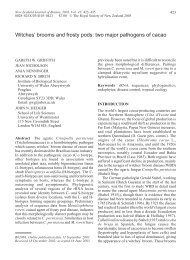
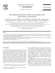
Fig. 1. The distance between images grabbed from a number of
regular positions and a target image at the centre of the area
The problem is then to compare images in a way that is
both fast and reliable and expresses this mapping between
images and positions. For this, we compare images using
a simple pixel-wise method. An h × w pixels image with c
colour components per pixel is a point in the image space, a
space having h × w × c dimensions representing all possible
images of the given size. Images can thus be compared by
measuring the distance between them in that image space.
In this work, for no other reason than simplicity, continuity
and smoothness, the Euclidean distance was used. The
distance between two images is thus defined as:
�
�
�
d(Ii, Ij) = � h×w � c�
(Ij(k, l) − Ii(k, l)) 2 , (1)
k=1 l=1
where Ii(k, l) and Ij(k, l) are the l th colour component of
the k th pixel of images Ii and Ij respectively. Pixels are
enumerated, without loss of generality, in raster order from
top-left corner to bottom-right corner. We used for this
work the RGB (Red-Green-Blue) colour space, thus having
three components per pixel. The combination of Euclidean
distance and RGB space is not necessarily the best to use
but it is sufficient for our purposes (see (Labrosse, 2006)
for a discussion).
Figure 1 shows the distance between a number of images
and a “target” image, in our Lab. The images were grabbed
from positions on a regular grid (81 images in total) and the
target image was grabbed from approximately the centre
of the grid. The grid size in Cartesian space is 4 m × 4 m.
For all the images the robot was facing the same direction.
Images corresponding to positions on Figure 1 around

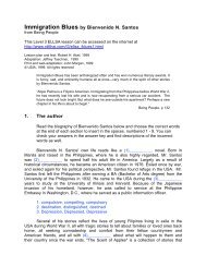
Fig. 2. Some of the images used for the experiment on Figure 1:
target image (top) and positions (3, 3.5) (middle) and (0, 0) (bottom)
It
Y
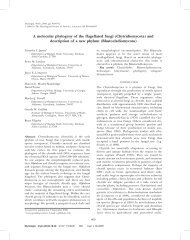
Fig. 3. The four images needed to compute the gradient of the
distance function at a given position
(0, 0) and (0, 4) were grabbed while the robot was almost
touching large objects (Figure 2, bottom), hence producing
larger and faster varying distance values compared to
other places where the robot was far from any object. This
is consistent with results presented in (Zeil et al., 2003) for
an outdoor environment in a large variety of spatial configurations.
The mapping between distance in image space (comparison
of the images) and in Cartesian space (distance to the
target) is clearly visible. In particular it is visible that the
homing position corresponds to the minimum of the distance
as a function of Cartesian space, which in a real situation
is not available. It is also clear that a gradient descent
on this function will lead to the minimum. This however implies
two problems: computing the gradient of the distance
function and knowing the orientation of the robot relative
to that of the target (the mapping is indeed not as clear
when the images are grabbed with random orientations).
Computing the gradient of the distance function at any
point requires four images: the target image It, the current
image Ic and two images Iδx and Iδy taken after two short
displacements from the current position corresponding to
two orthogonal directions X and Y , as shown in Figure 3.
A solution to that problem was proposed by Zeil et al.
(2003): physically moving the robot to obtain the images
Iδx and Iδy. However, in the context of mobile robotics this
is not desirable or even possible. It could be argued that
only a small triangular trajectory from the current position
is needed to obtain the three images, but such a trajectory
is difficult to accurately perform in all but contrived cases
and is impossible with many robots (but not with the one
Iδy
Ic
X
Iδx
3
we used in this work, although it was used as a car-like
vehicle, making such trajectory indeed difficult to follow).
Moreover, such a procedure would not be efficient, which
is important in many situations.
The problem of knowing the orientation of the robot relative
to that of the target can be solved in a number of ways
(and as such has been assumed to be available in many papers).
One solution is to use an additional sensor such as a
magnetic compass. Another is to incorporate the orientation
finding in the process. This is possible to some extent
for example as part of the feature matching process (Möller
et al., 1999) or optical flow computation (Röfer, 1997).
We propose our solution to these two problems in the
next section.
2.2. Our solution
The orientation of the robot can be estimated using the
panoramic images themselves. This is what we use here.
For each new image grabbed, the change in orientation is
computed by measuring column shifts between the previous
and current images (Labrosse, 2006). This procedure
provides the orientation of the robot at each new image
with an error within 20 ◦ after a long trajectory. For short
trajectories involved in homing, the typical error is below
5 ◦ , which is of the order of the maximum error the proposed
method can cope with (see (Binding and Labrosse, 2006)
for the relevant experiments).
Once the orientation of the robot relative to that of the
target is known, the direction of the two translations needed
for the gradient computation becomes specified.
We propose to simulate the translations by synthesising
the corresponding images from the current image Ic. There
is a large number of papers in the literature on image-based
rendering in general and simulation of new viewpoints in
particular. Most of these methods tackle the more general
and theoretical problems (Ullman and Basri, 1991; Lu
et al., 1998; Tenenbaum, 1998; Shum et al., 2002). In this
paper we adopt a more purposive approach because we are
only interested in simulating specific short displacements:
forward and sideways translations.
The environment of the robot projects onto the
panoramic images from left to right in the images as the
areas corresponding to the left of the robot (column 1),
the back (column 90), the right (column 180), the front
(column 270) and finally the left again (column 360), for
images that are 360 pixels wide, Figure 4. When the robot
moves forward, the part of the image corresponding to the
front of the robot expands while the part corresponding to

PSfrag replacements
Left Back Right Front Left
Fig. 4. Projection of the environment of the robot onto panoramic
images
Left Back Right Front Left
Left Back Right Front Left
Fig. 5. Deformations introduced in panoramic images by forward
(top) and sideways to the right (bottom) translation of the robot
the back contracts. The parts corresponding to the sides
move from front to back, Figure 5. A similar deformation
happens when the robot moves sideways (to the right).
An exact transformation could be computed using the
characteristics of the camera, if the 3D structure of the environment
was available. Indeed, the exact apparent motion
of objects in the images depends on their position in
the environment relative to the camera. Since the 3D structure
of the environment is not available, we can only compute
an approximation of the transformation. Moreover,
parts of the environment not visible from the current position
might be visible from the translated position, and
vice-versa. These occluded parts cannot be recovered by
any transformation of the images.
We perform the transformation by warping the images
using bilinear Coons patches (Heckbert, 1994). The method
only needs the boundary of the area of the original images
that need to be transformed into the new rectangular images,
this for both translations. To obtain these boundaries,
the rectangle corresponding to the boundary of the original
images is transformed as follows:
– the top and bottom edges of the rectangle are regularly
sampled into a number of positions x (20 in all the experiments
reported here);
– each position is shifted horizontally (sh) and vertically
(sv) using functions described below;
– the new positions are used as control points for the Coons
patches of the top and bottom parts of the boundaries;
– the right and left sides are defined by the extremities of
the top and bottom edges and are straight lines.
The two functions used to shift boundary positions are
4
Table 1
Parameters of the polynomials used for the warping corresponding
to a displacement of the robot of 25 cm
Parameter dh ah dv av
Value 3 3.0 3 1.2
piece-wise polynomials of the form s = ax d . These are characterised
by four parameters: dh and dv, and ah and av
respectively for the degrees and amplitudes of the polynomials
used for the horizontal and vertical shifts.
The value of the parameters was determined by optimisation
as follows. A number of pairs of images grabbed before
and after the short forward displacement to model was
acquired. For each pair, the first image was warped and
compared to the second image using Eq. (1) to obtain the
distance between the real and simulated images. This distance
was then minimised as a function of the amplitudes
of the polynomials for a range of values of the degrees of
the polynomials and the overall minimum was kept.
The degrees of the polynomials was not included in the
minimisation because of their discrete nature. Moreover,
because the image re-sampling operations (during acquisition
of the panoramic images and their warping) are done
without smoothing for efficiency reasons, the distance function
tends to present many flat steps separated by sharp
transitions. This means that the gradient of the function
to minimise is difficult to compute. The minimisation was
therefore done using the Nelder-Mead simplex method ∗ because
it does not need the gradient of the minimised function.
This minimisation was performed for a large number
of pairs of images and the average values was retained as
the parameters of the warping.
For the experiments reported here, the pairs of images
were taken for a forward displacement of 25 cm and the
optimal values obtained are given in Table 1. The degrees
of the polynomials has only very limited effect on the minimum
value obtained during the minimisation and on the
performance of the system. The amplitudes of the polynomials
is more critical as it reflects the amount of simulated
translation. The simulated displacement should be small
for the computed discrete gradients to be close to the real
gradient of the distance function between current and target
images. A displacement of the order of the displacement
between successive images while the robot moves is
appropriate. In previous work, the parameters were determined
manually and proved to simulate a (slightly wrong
and) too important displacement, making the estimation
∗ The implementation provided in the GNU Scientific Library was
used (http://www.gnu.org/software/gsl/).

sh
sv
3
0
-3
0
1
0
-1
0
90
90
180
Column index
Fig. 6. The functions used for the horizontal (top) and vertical
(bottom) shifts of positions to obtain the top of the boundary used
by the warping to simulate the forward translation. For the bottom
part of the boundary, the same functions were used but inverting
the column index.
180
Forward translation
Right translation
Fig. 7. The boundaries used by the warping to simulate the translations
(solid) that map onto the image (dashed)
Fig. 8. A pair of images used to determine the parameters of the
warping and the result of the warping: Ic (top), Iδx (middle) and the
simulation I ′ δx of Iδx (bottom). Vertical lines show the alignment of
several features.
of the gradient wrong, especially near the minimum of the
distance between current and target images, leading to the
systematic offset reported in (Binding and Labrosse, 2006).
Figure 6 shows the resulting functions that were used to
shift the boundary points. The sideways translation functions
are the same as for the forward translation but shifted
column-wise by 90 columns. Figure 7 shows the resulting
boundaries used by the warping.
Figure 8 shows an example of an image pair used to determine
the warping parameters along with the result of the
warping of the first image of the pair. Vertical lines show
the alignment of visual features of the images. This clearly
shows that the pixels of the real and simulated translations
align properly. Note that because the vertical shift is only
of 1.2 pixels, the effect of this shift is only barely visible
on Figure 7 and especially Figure 8. This has however a
definitive impact on the computed gradient.
270
270
360
360
5
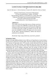
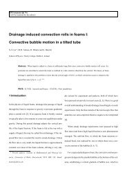
Fig. 9. The computed gradient for the images used in Figure 1
Once the images simulating the translation of the robot
can be obtained, the gradient of the distance function in
image space at the current position of the robot can be
computed using the current image Ic, the two simulated
images I ′ δx and I′ δy and the target image It:
Γ = (d(Ic, It) − d(I ′ δx, It), d(Ic, It) − d(I ′ δy, It)), (2)
assuming a unitary displacement. The gradient is a vector
the orientation of which, Θ(Γ), points towards the target. †
The gradient is expressed in the reference system of the
target, by aligning all images with the target, ‡ including any
specific orientation of the target that might not be null.
Figure 9 shows the gradient computed using the method
for the images used to compute the distance function in
Figure 1. This shows that the method works in most cases.
A typical failure is visible at the left corners of Figure 9.
These positions correspond to places in the environment
which were changing rapidly as a function of the displacement
of the robot because of the proximity of large objects,
Figure 2 (bottom). This is further discussed in Section 5.
It is interesting to note that, as expected from Figure 1,
the magnitude of the gradient increases dramatically as the
robot gets closer to the target. This will be used to compute
the rotational and translational speed of the robot.
Note as well that the computed gradient is much better
around the target than the one presented in (Binding and
† Actually, the gradient should point away from the target as it
should “indicate” high values of the distance function. However, for
convenience, the opposite value was adopted here.
‡ Note, however, that images need not be explicitly re-aligned. Instead,
a change in pixel indexing is performed for efficiency reasons.
Similarly, the warping is never explicitly performed but pre-computed
and saved in lookup tables.

Labrosse, 2006). This is due to the automatic estimation of
the parameters of the warping.
Aligning the robot with the direction provided by the
gradient would therefore make it move towards the target,
without knowing where the target or even the robot are in
Cartesian space. This is used for the homing step performed
in the central loop of the algorithm presented in Figure 10.
3. Long-range navigation: following way-images
3.1. From short to long-range navigation
The homing procedure directs the robot towards the target
following the angle Θ(Γ) of the gradient, from any position
at some distance away from it, withing the limits of
the performance of the controller of the robot.
Achieving long-range navigation is done by making the
robot “home” onto a succession of targets, or way-images.
If the gradient as computed in Section 2.2 was perfect, a
visual route would therefore be a linear approximation of
the real desired path.
However, as is visible in Figure 9 (and as the results will
show), the computed gradient is not necessarily pointing
directly at the target but rather follows local, possibly narrow,
valleys of the distance function. These narrow valleys
are created by asymmetries of the environment, in particular
sudden changes in appearance created by the proximity
of large objects. This implies that the actual path cannot be
guarantied. However, if the path is critical, more frequent
way-images can be used.
3.2. Route following: the algorithm
The algorithm to follow the succession of way-images
making up the route is detailed in Figure 10. The central
loop constitutes the “homing” step (reaching the next wayimage)
while the outer loop performs the following of the
succession of steps.
As previously stated, the orientation of the robot relative
to that of the target must be known at all times. Using
the visual compass (Labrosse, 2006), the orientation of the
robot at the beginning of the process must be available.
This is done by using a first way-image at the start of the
route. The robot grabs a first image and aligns it with the
way-image to compute its orientation relative to it. This is
done by minimising a function similar to the one shown in
Figure 1 but as a function of the orientation of the robot
rather than its position (Labrosse, 2006). Note that this
6
1: It ← firstWayImage()
2: Ic ← newImage()
3: initialiseOrientation(It,Ic)
2006)
4: while (moreWayImages()) do
// See (Labrosse,
5: It ← nextWayImage()
6: behindWayImage ← false
7: repeat // Homing loop
8: Ic ← newImage()
← forwardWarping(Ic)
9: I ′ 10:
δx
I ′ 11:
δy ← sidewaysWarping(Ic)
Γ ← gradient(It,Ic,I ′ δx ,I′ δy )
12: Θ ′ ← turningAngle()
13: τ ← translationSpeed(Γ)
14: ρ ← rotationSpeed(Θ ′ ,Γ)
15: robot.setSpeed(τ,ρ)
16: if (|Θ ′ | < θt) then
17: behindWayImage ← true
18: end if
19: until (behindWayImage && (|Θ ′ | > θT ))
image reached
// Way-
20: end while
21: alignRobot(It,Ic)
// End of route
Fig. 10. The visual route following algorithm
procedure does not need the robot to be precisely located
at the position of the first way-image.
A fixed speed was used all along the trajectory for normal
cruising, i.e. before reaching the last but one way-image.
When not at cruising speed, the magnitude of the gradient,
increasing when approaching a target, was used to set the
translational speed of the robot:
τ = τm/(1 + ||Γ||), (3)
where τm is a multiplicative factor. The speed was
clamped to a maximum value equal to the speed used
during normal cruising. This is implemented in function
translationSpeed().
The angle of the gradient is used to compute the turning
angle Θ ′ as the difference between the gradient direction
and the current orientation of the robot. This is then used
to compute the rotational speed. This speed could be a
simple proportion of the turning angle. However, because
the angle of the gradient is not reliable near the target (due
to the sudden change in the distance function at the target),
the rotational speed is set as:
ρ = ρm × Θ ′ /||Γ||, (4)
where ρm is a multiplicative factor. When the robot is far
from the target, the magnitude of the gradient tends to zero
and takes high values when nearing the target, values that
can be well above 1.0. In practise, because the magnitude

of the gradient can become very small, but never null, the
rotational speed is clamped to a maximum value to ensure
the robot cannot turn on the spot. This is implemented in
function rotationSpeed().
Determining when a way-image is reached can be done
in a number of ways. For example, as previously noted, the
magnitude of the gradient increases dramatically at the target.
A threshold on the magnitude, or its rate of change, or
on the distance itself could be used. However, such thresholds
are difficult to establish and their value depends on a
number of factors such as the pixel values of the images,
themselves depending on many factors (illumination, environment,
etc.).
We have used in (Binding and Labrosse, 2006) a sudden
change in gradient orientation to detect the passing of the
target, a method that has been used by others, e.g. Röfer
(1997). However, because the current implementation is
much faster than the previous, such sudden changes don’t
happen anymore in most cases. Instead, we simply keep
track of whether the robot has been behind the way-image
(absolute value of the turning angle less than a threshold
θt with a value of 50 ◦ in all experiments reported here) and
when this has been the case, then a turning angle becoming
higher than a threshold θT (set to 110 ◦ ) in absolute value
indicates that the robot just passed the target.
At the end of the route, the robot is aligned with the final
way-image by computing the difference in orientation between
the final way-image and the current image, as for the
initialisation of the orientation of the robot. Although this
only has a limited value for the route following, this shows
that should the visual compass used here drift (Labrosse,
2006), the orientation of the robot could be re-computed
when it passes way-images. This could systematically be
done to detect problems of the system, see Section 5. This
has not been done here.
4. Results
We report a number of experiments performed in our
Lab. The motion tracking system VICON 512 was used
to track the position and orientation of the robot during
the experiments to assess the precision, repeatability and
robustness of the method. All distances are given in metres.
Unless otherwise specified, the maximum speed of the robot
was set to 0.6 m/s, approximately the maximum speed the
robot can achieve, and turning rate to 28 ◦ /s. The robot used
was a Pioneer 2DXe equipped with a panoramic camera. All
the processing was performed on the on-board computer,
a Pentium III at 800 MHz.
7
2
1
0
-1
-2
-4
-2 0
2
4
Fig. 11. Homing from 18 different initial positions randomly scattered
around the target. The initial and final orientations of the robot are
show by short thin lines. The target is marked by a star.
As a rough measure of the cost of the computation, the
system was processing approximately 15 frames per second § ,
which is significantly faster than the slowest of two processing
speeds mentioned in (Stürzl and Mallot, 2006), but
on whole 2D images in our case. Finally, maximum speeds
were set such that the robot was not turning on the spot,
therefore approaching a car-like model, apart from during
the final alignment stage.
Often, during the experiments, users of the Lab moved
in view of the camera. This didn’t affect the performance of
the system, mostly because the projection of these people
in the images was small and therefore not consequential
when performing the global comparison of the images.
4.1. Homing experiments
We start with a number of homing experiments. The
reader is also directed to the experiments reported in (Binding
and Labrosse, 2006).
For the first experiment the target was positioned at the
centre of the play area to assess the performance of the
system when the robot starts from all around the target.
In all cases the robot started with the same orientation as
the target (within approximately 4 ◦ ). Figure 11 shows the
trajectories of the robot for 18 runs. The orientation of the
robot and target are shown with short thin lines. The target
is shown as a star.
All final positions are in a rectangle of about 1.5 m ×1 m
roughly centred on the target, compared to starting positions
as far as 4 m away from the target. The final orientation
is within 5 ◦ of the target orientation, which is approximately
the maximum error in initial orientation the
method coped with in an experiment reported in (Binding
§ The frame rate dropped to around 9 fps when the system was getting
VICON information due to the bottleneck of the communication
between the VICON server and the robot.

1
0
-1
-2
-2 -1 0
1
2
3
Fig. 12. Homing from 4 different initial positions 5.5 m away from
the target
and Labrosse, 2006). This shows a good repeatability of
the method. The performance seems however to be worse
than in (Binding and Labrosse, 2006). The starting positions
were however much further away from the target than
before. Moreover, in many cases, the robot finished further
away from the target than it was earlier on its path, as a
few highlighted cases in Figure 11 show. This indicates that
the stopping mechanism is not performing very well. Note
as well that the starting positions at the bottom of Figure
11 were approximately 50 cm away from obstacles and
with that respect the method performs much better than
in (Binding and Labrosse, 2006). Finally, and most importantly,
there is no bias in the homing position.
The second experiment shows the performance of the
homing over long distances. The target was set up at one
end of the play area and the robot started from 4 different
positions about 5.5 m away from the target. Because of the
many local minima of the distance function present over
such long distances, the robot did oscillate significantly. In
many cases this was triggering the finishing criterion, which
was therefore not used in this experiment. Rather, the robot
was manually stopped once it passed the target, the final
alignment therefore not being done. Despite the many local
minima, the robot does successfully reach the target with
a maximum distance to the target of about 60 cm.
The third experiment shows the repeatability of the trajectories.
The homing procedure was performed several
times from two different starting positions (with an initial
error within 28 mm in the x direction, 21 mm in the y direction
and 1 ◦ ). Figure 13 shows the results of the experiment.
All the trajectories finish less than 25 cm from the target
and the largest distance between trajectories is about
25 cm, these for initial positions about 3.5 m away from the
target. This shows good repeatability of the method.
8
1.5
0.5
-0.5
1
0
-1
-1.5
-1
2
1
0
-1
-2
-3
0
1
2 3
Fig. 13. Repeatability of the homing procedure
-2
-1
Fig. 14. Repeatability of the route following (1)
4.2. Route following experiments
Having shown the performance of the homing step, we
now present experiments on the long-range route following.
The first experiment uses 4 way-images set up as the vertices
of an approximate square, starting from the top left
corner and running clock-wise back to the starting position,
the first way-image being also used as the last. The route
was first followed 6 times from roughly the same pose (with
an accuracy similar to the one for the experiment on the
repeatability of the homing). The results are shown in Figure
14. A performance similar to that of the homing stage
is displayed. However, not visible on the figure is the fact
that the way-images were sometimes detected too late. One
such trajectory is highlighted in Figure 14. Although the
system did recover, this produced a significantly different
trajectory.
Figure 15 shows the same way-images but this time with
0
1
2

3
2
1
0
-1
-2
2
1
0
-1
-2
-3
-2
Fig. 15. Repeatability of the route following (2)
-2
0
Fig. 16. Repeatability of the route following on a long route
significantly different initial orientations of the robot. This
does lead to very different trajectories, mostly because
again of the late detection of the passing of the way-images.
Despite this, the robot still arrives in the vicinity of the
final way-image with the correct orientation.
The final experiment is a route made of 8 way-images,
is significantly longer, used most of the play area and was
indeed close to its edges (around 1 m at the bottom of Figure
16). The starting position was around (4, −0.5). Various
speeds and turning rates were used (maximum speeds from
0.3 m/s up to 0.6 m/s and maximum turning rates from
14 ◦ /s up to 28 ◦ /s, the highest values for both being the values
used for all the other experiments).
As with the previous experiments, the system did
wrongly detect the passing of way-images in a number of
cases. This was particularly the case of way-image 6 (at
position (0.25, −1.5)), which was detected just after pass-
-1
0
2
1
4
9
ing way-image 5. In one case (highlighted in Figure 16),
way-image 5 was detected while moving away from wayimage
6, therefore requiring a sudden change in orientation
to turn towards way-image 6. This triggered the detection
of way-image 6 while the robot was very far from it
(approximately at position (−2.7, −1.4)). Nevertheless,
the system recovered by simply moving onto the following
way-image.
However, it is visible that the accuracy does degrade significantly
as the robot progresses. This is partly due to the
increasing error in the measurement of the robot’s orientation
by the visual compass, mostly due to the fact that the
robot was moving close to some objects, which is the worst
situation for the visual compass (Labrosse, 2006) and for
the estimation of the gradient (Section 2.2). This suggests
that the orientation of the robot should indeed be updated
by aligning the current image with the way-image when its
passing is detected, Section 3.2. This however is not that
obvious, see Section 5.
5. Discussion
All the results show good performance of the visual homing
procedure and the long-range navigation proposed here.
In particular, good repeatability has been demonstrated.
The method makes a number of assumptions. The first
is that, at least for the final stage of the homing, the robot
must be able to turn on the spot. This is because no trajectory
planning has been incorporated in the procedure
to ensure that the robot arrives at the target with the correct
orientation. This is obviously a problem that needs
to be solved should the method be applied to a car-like
robot. However, reaching the correct orientation at each
way-image is not necessarily important and correct orientation
could be easily reached for the final target by specifying
a number of close sub-way-images just before the end
of the route. Smoothing the trajectories could however be
beneficial to ensure smooth transitions between segments
of trajectories at the passing of way-images. This moreover
might help solving the detection of this passing. This is still
work in progress.
The second assumption made by the method is that the
same parameters of the warping used to simulate the translation
of the robot for the gradient computation are suitable
in all situations. This is obviously wrong. For example,
the apparent motion of the objects in the images is more
important for objects that are close to the robot than for
far away objects. In other words, we use the “equal distance
assumption” that others have also used (Franz et al., 1998):

the robot is at the centre of a circular arena! However, the
parameters used in these experiments have been obtained
in an environment that was different (objects placed differently
around the play area) and for positions that were different
than the positions used in the reported experiments.
Despite this, the performance shown is good.
It is also not clear whether the warping should be symmetrical
for the front and back and for the right and left
because environments are usually not symmetrical around
the robot. This possibly means that the actual directions
of the simulated translations should probably be such that
they align with visual symmetries of the environment. Such
symmetries are however difficult to establish.
Because way-images can be in very different locations
for long-range navigation, establishing parameters on a per
way-image basis might be a good idea. This could be done
automatically from real images grabbed after a short (forward)
translation from the way-image, for example when
the route is saved by the robot during a tele-operated first
trip. However, automatically determining the parameters
of the sideways translation, if they need to be different from
that of the forward translation, might be a problem as many
robots cannot reliably perform that translation.
The third assumption is that the way-images can still be
obtained, which is not necessarily the case. For example
if the illumination is not constant in time, then images
grabbed during the route following will often not match the
way-images and the performance will decrease. It is however
possible to solve such problems by using different colour
spaces (Woodland and Labrosse, 2005) and using shadow
removal or colour constancy methods (Funt et al., 1992;
Finlayson et al., 1993; Barnard and Funt, 1998). Moreover,
it has been show that the combination of Euclidean distance
and RGB colour space is far from optimal (Labrosse, 2006).
This is an issue that still needs to be addressed.
More difficult to solve is the problem that the environment
of the robot might have changed between the acquisition
of the way-images and the route following. The system
is already robust to temporary changes in the current
appearance of the environment if these are not too significant.
This is partly because of the projection geometry of
the camera and the global nature of the image comparison,
partly because temporally short glitches do not affect
the system much. To cope with the stability of the wayimages,
it might be possible to replace single way-images
by several that would represent the variations of the appearance
of the environment at the corresponding position.
Methods such as the ones described by Neal and Labrosse
(2004) or Nehmzow and Vieira Neto (2006) might be useful
10
in that context. This would however imply more expensive
processing. More work is needed in that area.
Another improvement, as discussed above, might be to
re-align the visual compass with way-images when they
are passed by. This would reduce the drift of the visual
compass and/or would allow the detection of decreasing
performance. The problem is that if the robot passes (or
at least detects that it passes) a way-image while in fact
it is far from it, then the alignment of the current image
with the way-image is error-prone because of parallax error
(Labrosse, 2006). Doing so would therefore introduce wrong
corrections that might not have been needed.
Finally, the automatic creation of the visual routes could
also be important, in particular in the context of Simultaneous
Localisation And Mapping (SLAM). We have already
proposed methods to build topological maps (Neal
and Labrosse, 2004) but more needs to be done, in particular
taking into account the characteristics of the navigation
system.
6. Conclusion
We have described a method that uses simple 2D
panoramic image comparisons and techniques borrowed
from computer graphics to perform visual homing and
long-range navigation as a succession of homing steps.
The performance of the method has been evaluated in a
number of situations in our Lab and shown to be good. A
significant contribution of the work is to show that navigation
to a specified place in Cartesian space is possible
without knowing where the place is nor even where the
robot is. This has obvious applications, in particular in the
area of exploration and map building. Finally, the method
is fast and usually recovers from its own failures.
Acknowledgement
The equipment used for this work was partly funded by
HEFCW Science Research Investment Fund (SRIF) grants
from 1999 (for the VICON system) and 2002 (for the research
Lab and the robotic equipment).
References
Barnard, K., Funt, B., 1998. Experiments in sensor
sharpening for color constancy. In: Proceedings of the
IS&T/SID Sixth Color Imaging Conference: Color Science,
Systems and Applications.

Binding, D., Labrosse, F., 2006. Visual local navigation
using warped panoramic images. In: Proceedings of Towards
Autonomous Robotic Systems. University of Surrey,
Guildford, UK, pp. 19–26.
Bisset, D. L., Aldred, M. D., Wiseman, S. J., 2003.
Light detection apparatus. United States Patent
US 6,590,222 B1, also UK Patent GB 2 344 884 A, 2000.
Cartwright, B. A., Collett, T. S., 1983. Landmark learning
in bees: experiments and models. Journal of Comparative
Physiology 151, 521–543.
Cartwright, B. A., Collett, T. S., 1987. Landmark maps for
honeybees. Biological Cybernetics 57 (1/2), 85–93.
Finlayson, G. D., Drew, M. S., Funt, B. V., 1993. Diagonal
transforms suffice for color constancy. In: Proceedings of
the International Conference on Computer Vision. pp.
164–171.
Franz, M. O., Schölkopf, B., Mallot, H. A., Bülthoff, H. H.,
1998. Where did I take that snapshot? Scene-based homing
by image matching. Biological Cybernetics 79, 191–
202.
Funt, B. V., Drew, M. S., Brockington, M., 1992. Recovering
shading from color images. In: Proceedings of the
European Conference on Computer Vision. pp. 124–132.
Gonzales-Barbosa, J.-J., Lacroix, S., 2002. Rover localization
in natural environments by indexing panoramic images.
In: Proceedings of the IEEE International Conference
on Robotics and Automation. Washington, USA,
pp. 1365–1370.
Gourichon, S., 2004. Utilisation d’un compas visuel pour
la navigation d’un robot mobile. Ph.D. thesis, Université
Paris VI, Paris, France.
Heckbert, P. S., 1994. Bilinear Coons patch image warping.
In: Graphics Gems IV. Academic Press, pp. 438–446.
Labrosse, F., 2006. The visual compass: Performance and
limitations of an appearance-based method. Journal of
Field Robotics 23 (10), 913–941.
Lowe, D. G., 2004. Distinctive image features from scaleinvariant
keypoints. International Journal of Computer
Vision 60 (2), 91–110.
Lu, H.-m., Fainman, Y., Hecht-Nielsen, R., 1998. Image
manifolds. In: Proceedings of SPIE; Applications of Artificial
Neural Networks in Image Processing III. Vol. 3307.
San Jose, CA, USA, pp. 52–63.
Möller, R., Maris, M., Lambrinos, D., 1999. A neural model
of landmark navigation in insects. Neurocomputing 26–
27, 801–808.
Neal, M., Labrosse, F., 2004. Rotation-invariant appearance
based maps for robot navigation using an artificial
immune network algorithm. In: Proceedings of the
11
Congress on Evolutionary Computation. Vol. 1. Portland,
Oregon, USA, pp. 863–870.
Nehmzow, U., Vieira Neto, H., 2006. Visual attention and
novelty detection: Experiments with automatic scale selection.
In: Proceedings of Towards Autonomous Robotic
Systems. University of Surrey, Guildford, UK, pp. 139–
146.
Nistér, D., Naroditsky, O., Bergen, J., 2006. Visual odometry
for ground vehicle applications. Journal of Field
Robotics 23 (1).
Röfer, T., 1997. Controlling a wheelchair with image-based
homing. In: Proceedings of the AISB Symposium on Spatial
Reasoning in Mobile Robots and Animals. Manchester
University, UK.
Se, S., Lowe, D., Little, J., 2002. Mobile robot localization
and mapping with uncertainty using scale-invariant visual
landmarks. International Journal of Robotics Research
21 (8), 735–758.
Shum, H.-Y., Wang, L., Chai, J.-X., Tong, X., 2002. Rendering
by manifold hopping. International Journal of
Computer Vision 50 (2), 185–201.
Stürzl, W., Mallot, H. L., 2006. Efficient visual homing
based on Fourier transformed panoramic images. Journal
of Robotics and Autonomous Systems 54 (4), 300–313.
Tenenbaum, J. B., 1998. Mapping a manifold of perceptual
observations. Advances in Neural Information Processing
Systems (10).
Ullman, S., Basri, R., 1991. Recognition by linear combination
of models. IEEE Transactions on Pattern Analysis
and Machine Intelligence 13 (10), 992–1006.
Vardy, A., Oppacher, F., 2003. Low-level visual homing. In:
Advances in Artificial Life: Proceedings of the European
Conference on Artificial Life.
Vassallo, R. F., Santos-Victor, J., Schneebeli, H. J., 2002.
Using motor representations for topological mapping and
navigation. In: Proceedings of the International Conference
on Intelligent Robots and Systems. Lausanne,
Switzerland, pp. 478–483.
Woodland, A., Labrosse, F., 2005. On the separation of luminance
from colour in images. In: Proceedings of the
International Conference on Vision, Video, and Graphics.
University of Edinburgh, UK, pp. 29–36.
Zeil, J., Hofmann, M. I., Chahl, J. S., 2003. Catchment
areas of panoramic snapshots in outdoor scenes. Journal
of the Optical Society of America A 20 (3), 450–469.