1U08p2c

SERC DISCUSSION PAPER 197
Enabled to Work:
The Impact of
Government
Housing on Slum
Dwellers in
South Africa
Simon Franklin (SERC)
May 2016

This work is part of the research programme of the UK Spatial Economics Research
Centre funded by a grant from the Economic and Social Research Council (ESRC).
The views expressed are those of the authors and do not represent the views of the
ESRC.
© S. Franklin, submitted 2016

Enabled to Work: The Impact of Government Housing on
Slum Dwellers in South Africa
Simon Franklin*
May 2016
* Spatial Economics Research Centre and London School of Economics
This paper is a part of a Global Research Program on Spatial Development of Cities, funded
by the Multi Donor Trust Fund on Sustainable Urbanization of the World Bank and supported
by the UK Department for International Development. For their assistance in giving me
access to specific household GIS data and an early release of the 5th wave of CAPS data, I’d
like to thank Jeremy Seekings, Brendan Maughan-Brown and David Lam. Thank you to
Magdalen College for providing a great deal of the funding that made possible my research in
Cape Town. Thank you to Marcel Fafchamps for input, oversight and guidance of the project.
Thank you to helpful seminar participants at the CSAE Conference, Oxford OXIGED
housing workshop, as well various internal seminars in Oxford. In particular I thank Tony
Venables, Stefan Dercon, Paul Collier, Somik Lall, John Muellbauer, Taryn Dinkelman,
James Fenske, Simon Quinn, Francis Teal, Julien Labonne, & Kate Vyborny. I also thank
two anonymous MPhil examiners for their detailed and useful comments.

Abstract
This paper looks at the link between housing conditions and household income and labour
market participation in South Africa. I use four waves of panel data from 2002-2009 on
households that were originally living in informal dwellings. I find that those households that
received free government housing later experienced large increases in their incomes. This
effect is driven by increased employment rates among female members of these households,
rather than other sources of income. I take advantage of a natural experiment created by a
policy of allocating housing to households that lived in close proximity to new housing
developments. Using rich spatial data on the roll out of government housing projects, I
generate geographic instruments to predict selection into receiving housing. I then use
housing projects that were planned and approved but never actually built to allay concerns
about non-random placement of housing projects. The fixed effects results are robust to the
use of these instruments and placebo tests. I present suggestive evidence that formal housing
alleviates the demands of work at home for women, which leads to increases in labour supply
to wage paying jobs.
Keywords: housing, labour supply, time allocation, home production
JEL Classifications: P14; J22; O18; D13

1 Introduction
Substandard housing conditions are considered to be one of the key deprivations suffered by the
poor. Currently, it is estimated that over 860 million people live in slums in developing countries,
and this number has been growing rapidly over the last decade (UN Habitat, 2003, 2010). Living
in informal settlements is associated with a lack of access to running water, electricity, ventilation,
security of tenure and access to economic opportunity. Improving or eradicating slums has been
a key policy goal of governments, yet there is no clear consensus on what best practice should
be. 1 Slums can be thought to constitute a poverty trap (Marx et al., 2013). Living in a slum is not
only an outcome of poverty, a growing body of evidence shows that slum conditions themselves
have a detrimental impact on households. Yet improving housing conditions at the cost of
relocating households further away from jobs and existing networks could do more harm than
good (Barnhardt et al., 2014; Lall et al., 2008). Policies aimed at improving the housing conditions
of the poor need to take account the effect that they have on the economic and labour outcomes
of slum-dwellers.
This paper examines the links between housing conditions and labour supply. Over the past
20 years the South African government has provided over 3 million free stand-alone houses to
its citizens. While the government housing policy has been praised for the extraordinary scale
of delivery of housing, it has also been criticised for providing low quality homes in areas far
away from jobs. I study the impact of free government housing in South Africa, and find clear
evidence of increased incomes among recipient households. The evidence suggests that poor
housing conditions constrain the ability of households to take wage-paying work.
I use longitudinal household data from Cape Town over four waves from 2002 to 2009 to assess
the impact of government housing on household income and labour market participation. 2 I test
the hypothesis that receiving a government home allows substitution from labour at home to
work in the labour market, which in turn leads to increases in household income.
I use the allocation procedure used by the local government to award housing to households
as a natural experiment. Recipients of housing were selected because of their proximity to the
new housing projects. I proceed in two steps: firstly I use the distance between households’
original place of living and locations of newly built housing projects to instrument for individual
selection into treatment. To do this I develop a unique maximum likelihood estimator
which predicts the probability of receiving government housing from any one of multiple nearby
housing projects.
Secondly, I control for non-random locations for the selected sites of new housing projects. I
use a set of housing projects that were approved and planned but cancelled for reasons unrelated
to the communities they were intended to benefit. I exclude from the sample households that
had no projects planned nearby and use only those households that had planned but incomplete
projects nearby as a control group. I then repeat the main estimates using only completed
projects as instruments.
Both household fixed effects and instrumental variable estimates show that households receiving
government housing experience large increases in income, relative to households that do not
receive housing. These findings are robust to tests using the cancelled projects. In general the IV
1 For an overview of some of the debates in this literature see Marx et al. (2013); Collier and Venables (2013); Davis
(2007); Werlin (1999).
2 It is estimated that between one quarter and one fifth Cape Town’s entire population benefited from government
housing since 1994 (Seekings et al., 2010).
2

esults are larger than the fixed-effects results. This is consistent either with measurement error,
or a story whereby households with the greatest needs (those struggling economically) within
communities are awarded the housing, leading to downward bias in the fixed-effect estimates. 3
I investigate the channels through which improved housing increases household incomes. I
find that the rise in household income is due to wage employment, rather than increases in
income from rent or self-employment. The effect seems to be driven by increased female labour
force participation. Women in treated households are more likely to be working in wage labour.
These effects are not present for male households members. However, I do find a significant
treatment effect on both both female and male household members’ wage earnings.
The concentration of the effect on female labour supply suggests that poor housing conditions
place particular burdens on the time use of women. I show that that women in South Africa,
particularly in informal settlements, allocate significant time to housework and care. This is
consistent with evidence from other developing countries (Berniell and Sánchez-Páramo, 2012).
Due to data limitations, I cannot conclusively show that this is the main channel driving the
results. I do find that government housing significantly increases electrification, direct access to
running water, and modern home appliances, all of which could be saving significant amounts
of time for women. In addition, living in the South African slums is hazardous- shack fires are
common because of low quality stove and heating devices. I speculate that improved housing
could reduce time mending and rebuilding after these kinds of disasters.
Field (2007) argues that improved tenure security frees up time that otherwise would have
been spent at home defending the home from expropriation. Most South African households in
informal settlements already enjoy de-facto tenure security (Payne et al., 2008), and eviction risks
that do exist are unlikely to be bolstered by time spent at home. 4 I argue that these results are
not driven by tenure security. Instead, South African households face a high rate of crime, and
may need to spend time at home to deter intruders. I show that receiving government housing
significantly increases feelings of safety in the home.
I contribute to the literature on the relationship between physical living conditions and female
labour supply. Labour saving improvements to the lives of the poor can free up time to work
in the labour market (Duflo, 2012; Greenwood et al., 2005; Devoto et al., 2011). Dinkelman
(2011) and Field (2007) show that home electrification and improved tenure security, respectively,
increase female labour supply and earnings by freeing up time from work at home. In the context
of housing projects specifically, Keare and Parris (1982) find that provision of tenure and basic
services in four countries had positive impacts on employment and income generation.
A related literature looks at the impact of where people live on their labour outcomes (Bryan
et al., 2014; Ardington et al., 2009; Barnhardt et al., 2014; Franklin, 2015). The housing project
studied in this paper moved households very slightly further away from job opportunities. In
a setting where distance from jobs is thought to be an important contributor to poor labour
market outcomes for black South Africans (Banerjee et al., 2007), I find evidence that government
housing is not improving the class and race-based segregation of the city. My study benefits from
an IV estimator that estimates the impacts of housing on those that did not have to move too far.
In this way my study isolates the impact of housing on household outcomes from the effect of
3 It could be because of local average treatment effect interpretation of the results, which I discuss in detail in the
paper. Briefly, the instruments identify the effect on households that didn’t have to move too far to take up housing,
because they were treated by virtue of their proximity to housing.
4 Ironically, evictions that have come from large townships, as opposed to “squatter” settlements on private land,
are made by the government to make way for government housing projects. While these evictions often come with
the promise of replacement government housing, some households could miss out, or have been placed in temporary
shelters for long periods of time.
3

elocation. 5
Secondly, I contribute to the broader literature on the ways in which slum living constitutes
a poverty trap. A growing literature looks at the impact of slum upgrading on health and wellbeing
(Cattaneo et al., 2009; Galiani et al., 2014), considerable evidence shows large impacts on
health of improved access to services such as sanitation and running water (Zwane and Kremer,
2007; Pitt et al., 2006; Jalan and Ravallion, 2003; Duflo et al., 2012). Marx et al. (2013) discuss
three channels through which slums could act as a poverty trap: human capital and health
effects, poor incentives for policy, and under-investment due to weak property rights. 6 I add a
forth channel to this list by showing that poor housing conditions can constraint labour market
participation.
Thirdly, this paper provides a rigorous evaluation of a large scale government program that
is the subject of much debate and criticism. The scale and political sensitivities of projects like
these make them difficult to randomize. A large developed country literature generally draws
negative conclusions about the impacts of large scale public housing projects (Olsen and Zabel,
2014). 7 This is the first rigorous evaluation, to my knowledge, of a housing project that provides
a complete housing unit free of charge in developing country context.
Indeed, delivery of housing on the scale of millions of households is usually considered infeasible
or not cost-effective for most developing countries (Gilbert, 2004). Donors and researchers
have tended to focus on evaluations of upgrading and land-titling programs. However, standard
policy approaches have had little success at mitigating the expansion of slums (Marx et al., 2013).
Housing projects of the kind of implemented by South Africa are popular with governments, because
they are so popular with electorates. Ethiopia and Columbia (Gilbert, 2014) are embarking
on a housing projects of a similar scale. Rigorous evaluations of projects like these are important
to guide policy makers, to inform best practices for dealing with informal housing conditions.
Finally I contribute methodologically to a growing literature that attempts to estimate the
effects of housing policies and urban policy more generally (Baum-Snow and Ferreira, 2014;
Field and Kremer, 2006). Local area instrumental variables are harder to use in a setting of
continuous population density. I extend a literature that uses proximity data to instrument for
individual selection into projects (Attanasio and Vera-Hernandez, 2004; McKenzie and Seynabou
Sakho, 2010). I overcome the challenge of multiple weak instruments and improve the efficiency
of my first stage IV estimate by creating a unique maximum likelihood estimator for the effect
to create a time-varying set of instruments top predict selection into housing.
The rest of the paper is organized as follows. In Section 2 I discuss the context of housing
policy in South Africa, as well the role of work at home for women in South Africa. I present a
simple model of how housing could increase labour supply for women. Section 3 describes the
GIS and survey data used in the paper. In Section 4 I describe the instrumental variables strategy
in detail, and show results from the first stage to show that proximity to housing predicts selection
into treatment. Section 5 show the main results for household earnings. The mechanisms
driving the impacts on income are discussed in Section 6, while further robustness checks are in
Section 7. Section 8 concludes.
5 If the movement induced by housing did have negative impacts on household outcomes, it seems that household
incomes rise in spite of this additional distance from jobs.
6 Galiani and Schargrodsky (2010) provide strong evidence for the last of these channels in Argentina.
7 The flavour of these arguments are still best summarized by Jane Jacobs (1961), in her seminal text on urban planning:
“The method fails. At best it merely shifts slums from here to there, adding its own tincture of extra hardship and
disruption. At worst, it destroys neighbourhoods where constructive and improving communities exist and where the
situation calls for encouragement rather than destruction”.
4

2 Setting and Context
Informal settlements in South Africa grew in the context of the apartheid system of enforced
segregation. Relocation of non-white populations to the periphery of cities or remote rural
areas has left a persistent pattern of segregation. Poor non-white areas are located far from
more prosperous city centres. Migrant labour in cities was highly regulated, making access to
urban employment a constant battle, and secure rights to adequate housing in the cities almost
impossible (Royston, 1998). Public investment in urban infrastructure and housing in black areas
was minimal.
As the architecture of apartheid was dismantled, starting in the 1980’s with the repeal of the
Group Areas Act, families that had previously been prevented from doing so began to move to
the cities in vast numbers. This rate of migration, combined with the poor existing housing stock
and South Africa’s extremely high and rising employment rate (estimated to be around 24% for
those actively seeking work) has led to a housing crisis. Many new urban migrants moved into
shacks built in the backyards of existing formal dwellers (Seekings et al., 2010).
When the first democratic government was elected in 1994 there were an estimated 12.5 million
people without adequate housing. Only 65% of the total population was housed in formal
(cement and brick) dwellings, and high household formation rates have made this problem even
more acute. It is estimated that the number of informal dwellings in Cape Town grew from 28
000 in 1993 to roughly 100 000 in 2005 under the pressure of migration and urban population
growth (Rodriques et al., 2006).
2.1 Housing Policy
The first democratically elected government embarked on a number of policies to improve the
lives of South Africans. 8 The new South African constitution included the right to adequate
housing (see Section 26, Constitution of South Africa). 9 The South African government promised
to deliver 1 million houses in the 5 years between 1995 and 2000. This ambitious target was more
or less met. By 2008 it was estimated that 2.3 million houses had been built, and in May 2013
the government announced that it had passed the 3 million mark (South Africa, 2013). 10
This housing policy, originally referred to as the Reconstruction and Development Program
(RDP) aimed to provide as many low cost houses as quickly as possible. 11 The value of the house
provided is very small in comparison to similar projects in countries such as Chile (Gilbert, 2004).
The program gives individual capital subsidies to eligible households. However, the vast
majority of the subsidies have been product linked; they had to be used to purchase houses
commissioned by the government and built by private construction companies. These came
to be known as the RDP houses, small stand alone units built on large empty land just outside
existing informal settlements. Government housing policy was updated with the “Breaking
New Ground” policy document of 2004, which placed increased emphasis on minimum build-
8 Important policies include electrification of 1.75 million home, improved access to running water to nearly 5 million
people in rural areas, the extension of free basic health care to 5 million people, and a childcare grant and pension
program. Some evidence on the positive impacts of these policies are documented in Duflo (2003); Case and Deaton
(1998); Dinkelman (2011).
9 The South African constitutional court has consistently upheld individual rights to housing, and these constitutional
changes have insured rights to land for millions of households that were previously categorized as “squatters”. For a
description of the watershed legal case involving land rights see Sachs (2003) on the Grootboom case.
10 According to the census of 2011 there are approximately 14.5 million households in total in South Africa.
11 This policy of the national housing subsidy scheme was outlined in “A New Housing Policy and Strategy for South
Africa” (Republic of South Africa, 1994).
5

ing standards, in situ approaches to upgrading, rental housing and densification (Charlton and
Kihato, 2006). But by and large, the housing scheme has continued to be characterized by the
construction of large greenfields projects. Small houses on separate plots with the orange roofs
that have come to characterize the South African urban landscape. For a detailed and up-to-date
outline of issues relating to the housing policy, see Tissington (2011). There is no evidence to
my knowledge that government housing projects have been rolled out in conjunction with other
welfare or urban improvements projects.
To be eligible to receive housing an individual applicant needs to be married or otherwise
supporting dependents in a household with total income of less than R3500 per month, cannot
own a registered property, and must be a South African citizen (Department of Human
Settlements, 2009). 12
The success in the delivery of housing units has been a cornerstone of the African National
Congress’s electoral campaigns since 1994. More than 10 million people are estimated to have
benefited directly from the program. Yet in a period of increasing poverty, unemployment and
urbanization, the number of households living in informal housing has actually increased, especially
among the African population.
The policy has been criticised for not doing enough to deal with the housing backlog, providing
low quality substandard housing that hardly improves living conditions of the poor (Tomlinson,
1998; Lipman, 1998), not being accompanied with other infrastructure and neighbourhood
investments (Huchzermeyer, 2003) and for not doing enough to deal informality by ensuring
transfer of title deeds (Huchzermeyer and Karam, 2006). Housing programs have been said to
have contributed to forced evictions (Chance, 2008), particularly to areas further away (Centre
on Housing Rights and Evictions, 2009) and to have been biased towards particular racial or
political groups (Seekings et al., 2010). The most pervasive criticism of the policy has been the
location of housing which has often been determined by private construction companies that
choose to build on the cheapest possible land. In most cities housing has been built far away
from the city centres in a way that has reinforced the spatial segregation of South African cities
(Huchzermeyer, 2006; Bundy, 2014; Charlton and Kihato, 2006).
In the setting where this study is conducted, the Western Cape Occupancy Study (Vorster
and Tolken, 2008) finds that resale rates of housing are high, at around 20%, mostly on an
informal market. Rental of these houses does not appear to be at all common, while the practice
of building a small “backyard” shack or shelter is. More than one third of households had a
backyard structure within a few years of receiving the house. 13
While many studies have evaluated government housing using observational data or qualitative
analysis, there is no study, to my knowledge, that attempts to estimate causal impacts of
government houses on the outcomes of households receiving them.
2.2 Theoretical Framework
In this section, I provide a theoretical basis for causal links between housing and household
labour participation. I provide evidence on the patterns of time use for female household mem-
12 It has been frequently observed that these eligibility requirements were often unverified, and for the vast majority of
slum dwellers, are not likely to be binding anyway. I discuss issues to do with allocation of housing to applicants when
I discuss the identification strategy used in this paper in Section 4
13 These structure were sometimes used to accommodate other members of the household that could not fit in the
original structure. In the cases when the structures were occupied by non-household members, only about half of paid
rent. Some households still owned their previous (informal) dwelling, and were renting it out, but in most cases their
informal dwellings had been demolished when they left, or they had given it to a friend or family member.
6

ers in South Africa and argue that slum dwellers’ time is constrained by their physical living
environment. A simple model of home production predicts that upgrading housing would induce
substitution of time away from home production into wage labour.
I conceive of home production as time consuming activities related to the production of goods
and services consumed at home. This includes maintaining the physical structure to ensure
safety, security, warmth and shelter, household activities such as cooking and cleaning, and
rebuilding of structures after damage from fires or flooding.
The UN-Habitat report of 2003 (UN Habitat, 2003) outlines a full taxonomy of the basic characteristics
of slums. Many of the deprivations of slum living relate to issues of home production.
Cooking and bathing is likely to be considerably easier in a home with running water and electricity,
as opposed to a informal dwelling where other carbon fuel sources are often collected,
and water has to be fetched from communal taps. Maintaining a sanitary home environment is
also likely to be far easier in a cement floored home without leaking roofs or permeable walls. 14
In Cape Town most slum dwellers have to use badly maintained communal toilets located some
distance from their homes, or buckets which must be emptied outside of the home every morning.
Paraffin is a common use of fuel for cooking and heating, and is known to be a cause of fires
and respiratory disease (Schwebel et al., 2009). In Cape Town, as in slums around the world,
formal electricity connections are rare for shack dwellers, with more than 50% having fire-prone
illegal connections, or no electricity at all (City of Cape Town, 2005). Electricity greatly aides
home production if it facilitates the use of fridges, stoves and microwaves.
Time use surveys of poor South African indicate that a considerable amount of time is consumed
by domestic activities, particularly for female members of households, who are primarily
responsible for chores at home. South African women spend on average three times as long (3.5
hours a day) as men on unpaid work (Budlender et al., 2001). 15 Crucially, the evidence suggests
that these activities take far longer in informal housing. In the national accounts individuals
living in informal housing in urban areas spent 25% more time on non-labour market work
than other urban households (Budlender et al., 2001). Shack dwellers in Cape Town report more
than twice as much time (17.1 hours per week) spent on housework than their formally housed
counterparts (7.5 hours per week). 16
Many of the issues related to time use are likely to do with access to labour saving appliances.
In 2000 only 28% of informal dwellings in urban areas used electricity for cooking, versus 77% of
urban households. Similarly they were far more likely to use gas or paraffin stoves for cooking
and heating and lighting. Only 46% of shack dwellers have access to a refrigerator, compared to
90% of families in brick houses.
Households living in the slums on the Cape flats are extremely vulnerable to township fires
and, during winter months, storms and flooding. 17 Fire hazards are due, in part, to the types
of appliances used for cooking and heating outlined above. These events are common, and
often lead to widespread destruction of housing infrastructure, which takes time and money to
rebuild.
14 Cattaneo et al. (2009) have looked at how cement floors improve health from improved sanitary conditions.
15 These patterns are consistent estimates for other developing countries (Berniell and Sánchez-Páramo, 2012).
16 These were calculations based on the CAPS datasets used for this paper, outlined in Section 3. Unfortunately this
data was no collected for periods of the survey beyond the first wave, which makes it impossible to estimate the impact
of housing on time use in this setting.
17 In 2005 a particularly damaging fire razed over 3000 shacks in Joe Slovo informal settlement just outside of Cape
Town (“Shack-dwellers have nothing left after blaze” (iolnews, January 17 2005)) The victims of the fire were promised
government housing after being displaced, but many remain in temporary relocation camps years later (Centre on
Housing Rights and Evictions, 2009).
7

Pharoah (2012) provides an overview of some of the risks facing informal dwellers in Cape
Town. The greatest impacts come from the health problems and losses of days worked and at
school because of the disruption caused by fires. 18 In that study 83% of shack dwellers had
experienced some kind of flooding while living in Cape Town.
In addition, slum dwellers have considerably less security, since their homes can easily be
broken into. This could impose limits on tenants’ ability to commute into the city to look for
work for fear of theft. 19
2.3 A Model of Home Production, Work and Leisure
All told, the time burdens of living in informal dwellings are considerable. In the empirical
analysis I seek to evaluate the total effect of receiving housing, which affects the way in which
home production happens through many channels. In what follows, I present a simple model
of how changes in housing quality could influence home production, which in turn predicts
increases in labour hours due to the effect of formalized housing. I do not distinguish between
the different channels through which housing could improve home production, which were
outlined in the previous section.
The model I use is of the lineage of Becker (1965), since it specifies utility as a function of
an unobserved home production input H(T h , b), which is produced through time at home T h
in combination with the physical housing infrastructure b. Importantly, I assume that home
produced goods and services are not perfect substitutes with other forms of consumption, as
opposed to many of the other models in this literature (Gronau, 1977, for example). This fits
with the way I have conceived of home production in informal settings, where the basic needs
provided for by housing cannot be taken for granted.
In this model, production at home cannot be traded on the market, it is used within the household.
Household utility is a function of home production, consumption and leisure U(H, C, L).
Consumption is given by time spent working for wage labour T w times the prevailing wage w.
Leisure, time on home production, and time at work sum to one. With prices normalized to one,
household utility is given by:
U(H(T h , b), wT w , 1 − T h − T w , )
If the household maximizes utility with respect to its allocation of time between labour, leisure
and work at home, the first order conditions are simple:
U H · H Th = U L
U C · w = U L
The optimizing household would thus choose its optimal time on work at home and labour,
given by Th ⋆ = T⋆ h (b, w) and T⋆ w = Tw(b, ⋆ w), respectively. I want to find dT⋆ w
db
: the impact of
upgrading the physical housing infrastructure on wage labour supplied. While one could speculate
intuitively about the direction of impact from the FOC’s, total differentiation with respect
18 Some 20% of live in high flood risk areas, and roughly 40 000 people were directly affected by townships fires in
Cape Town between 1995 and 2004.
19 This threat of invasion seems more urgent than that of expropriation risk (Field, 2007). While security of tenure is
a great issue for informal dwellers in South Africa (Royston, 2002) this risk is related more to formal eviction to make
way for new housing or urban development projects, rather than contestation of property right by other private agents.
8

to b, gives a more complete picture, in the general case. With some manipulation this eventually
yields:
dT ⋆ w
db
[
U LL − wU ]
CC + U LL
(U LL + U HH H T + H TT U H ) = −[U HH H
U b H T + H Tb U H ]
LL
dT ⋆ w
db = [U HH H b H t + H Tb U H ]
wU CC +
(
UCC w+U LL
U LL
)
(U HH H T + H TT U H )
Assuming diminishing marginal utility for all inputs into the utility function, and a diminishing
marginal product of time at home, renders the denominator unambiguously negative. Turning
to the numerator, the first term is clearly negative due to the diminishing marginal returns on
home production and the positive returns to housing quality from time spent at home. The sign
of the second term hinges on whether or not the marginal utility of time in the home increases
or decreases with an improvement in housing quality. If H Tb = ∂2 H
∂T∂b
≤ 0 the numerator would
be negative, and the response of hours in the labour market would be unambiguously positive.
The sign of the H Tb reflects the extent to which the returns to time spent on activities in
the home increase or decrease as the home technology improves. In an setting where home
production leads to income through the production of goods sold on the market, one might
expect a positive sign for H Tb : b acts as production technology that allows households to increase
output by working at home more.
I would argue that under my definition of home production, H Tb is likely to be negative in
this context. Improved housing is thought to be a labour saving technology, allowing households
to reach a desired level of home quality. For instance, providing a better roof and walls would
reduce the value of work done on maintaining the home, because nothing really needs to be
done to make the structure more secure anymore.
In a sense, the empirical results of the paper provide a test of the sign of H Tb , showing that
poor housing quality necessitates increased time spent at home, which could be spent more
productivity somewhere else.
2.3.1 Alternative channels
I cannot rule rule out other channels that could lead to changes in household labour supply.
Health could be leading to a positive impact on labour supply through the productivity of
household members. There is a large literature looking at the links between health and productivity
(Strauss, 1986; Strauss and Thomas, 1998). The links between housing and health are also
firmly established (Pitt et al., 2006; Cattaneo et al., 2009). This channel is relevant in this setting,
but I am unable to estimate the impact of housing on health using the data available. Given that
the impacts of improved health are likely to accrue more to female members of households who
spend the most time using the stoves and appliances that are most detrimental to health, this
effect might be considered part of the full effect of informal housing on female capabilities.
In addition there could be additional effects of receiving government housing such as changes
in household composition, new rental income, and household location. New household members
might move into the additional space that a larger house and plot affords. These new
arrivals could bring with them sources of income if they are employed, or government grants.
Alternatively they could be alleviating the burden of work in the home, allowing other members
9

of the household to seek employment. Recipients of housing could see large increases in incomes
due to rental incomes- either from the shacks they have moved out of, or backyard structures
constructed on their properties, which is common practice. 20 In my empirical analysis I will
show that the results are not influenced by including controls for changes in household size
and composition, nor are they effected by looking at per capita measures of household income
and earnings. I argue that the labour supply channel fully explains the impacts on household
income.
3 Data
My empirical analysis uses the CAPS panel survey of Cape Town metropolitan area, with four
waves collected in 2002, 2005, 2006, and 2009. 21 The sample was randomly selected using probability
proportional to size sampling and stratification by racial group using 1996 local area
census data. 22
Of the households surveyed in the first wave, roughly one third were living in informal
dwellings. For the purposes of evaluating the impact of receiving a housing subsidy, it was
necessary to drop all those who weren’t eligible, and therefore not a valid control group. As a
result I have dropped all households that were not living in an informal dwelling (or “shack” as
coded in my data). I also drop the few households who report that they have already received
government housing before wave one. Households who have received government housing are
usually not still living in shacks, but some have moved out or lost their houses. These individuals
are no longer eligible for housing and thus should not be in the sample. This leaves me with a
sample of 1350 eligible households. 1097 of these are found at least once in subsequent waves. 23
Table 1 provides an overview of my sample of houses that were living in shacks in 2002. Over
a period of just 7 years nearly 40% of the sample has received a government house. I show the
proportion of households that received housing for each wave of data (“Treated Here”) as well
as cumulative proportion that have received housing to that point. It is the latter outcome that
will be used as the dependent variable in the analysis because I expect the impact of housing
to be present in all periods after which it is received. More households are treated between the
first and second periods (19.7%) than any other. The high proportion of households receiving
housing in this data is testament to the scale of the roll out of the housing program in Cape
Town.
However, it is also striking how rapidly all households improved the quality of their living
and housing conditions. Some of this effect is undoubtedly due to government housing, but
households that did not receive government housing managed to either improve their housing
20 Rent and one off wealth increases from the sale of housing should not be included in measures of include, but it is
possible that these were incorrectly reported by households.
21 The Cape Area Panel Study Waves 1-2-3 were collected between 2002 and 2005 by the University of Cape Town
and the University of Michigan, with funding provided by the US National Institute for Child Health and Human
Development and the Andrew W. Mellon Foundation. Wave 4 was collected in 2006 by the University of Cape Town,
University of Michigan and Princeton University. Major funding for Wave 4 was provided by the National Institute on
Aging through a grant to Princeton University, in addition to funding provided by NICHD through the University of
Michigan (Lam et al., 2006). Further information can be found on the CAPS website at http://www.caps.uct.ac.za
22 This survey was conducted with the primary motivation of tracking young adult’s behaviour, sexual attitudes, labour
force participation and health. However household questionnaires were also conducted, with an extensive household
roster questionnaire which surveyed the entire household. However, this does impose some limitations on the analysis
that can be conducted.
23 Although in each specific follow up wave about 80% of households are reached on average, conditional on having
been found at least once in the follow up waves.
10

conditions (move out of shacks) or gain access to important infrastructure and amenities. This
could be due to both improved government service delivery during this time, and a natural
process whereby new migrants to cities manage to improve their living conditions over time,
consistent with a “modernization theory of slums” (Marx et al., 2013). Indeed many of the
households in informal housing in the first wave of the panel were recent migrants to the city.
Table 1: Evolution of sample household characteristics
Wave 1 2 3 4
Year 2002 2005 2006 2009
Treated 0.0% 19.7% 25.9% 38.6%
Treated Here 0.0% 19.7% 8.87% 12.09%
Shack 100.0% 65.6% 62.4% 45.6%
Flush Toilet 70.8% 79.2% 85.6% 90.7%
Piped Water 12.3% 25.3% 28.4% 42.0%
% Female 54.0% 55.1% 54.0% 53.3%
Dist To City (km) 23.51 23.69 23.65 23.55
Head of Household Background
Coloured 15.0%
African 83.2%
Moved to Cape Since 1985 56.2%
Born Cape Town 19.0%
Born Eastern Cape 75.1%
Lived in backyard dwelling 10.6%
The scale of rollout of housing, the effects of which are clear in my sample, provides a perfect
setting in which to evaluate the effects of government housing on labour outcomes. My data
includes information on housing conditions in each wave of the survey, and detailed information
on labour market decisions of one young adult member of the household. Other labour data
comes from the household rosters.
In Table 19 in the Appendix, I compare the sample mean for households that received housing
to those that did not at both baseline and and endline (at baseline I look at househld that are
going to receive housing). There are clear differences in observables between treated and control
individuals. This differences are consistent with a story of housing allocation whereby poorer
households were more likely to get housing, as discussed in Section 4. Backyarders (those living
not in large informal settlements but in shacks in the yards of a more formal dwellings) seem far
less likely to get housing, as are coloured households. Migrant status does not seem to make a
significant difference. Importantly, we observe that households that were treated lived far further
away from the city center, which is due to to fact that projects were built further away from the
city, where there was more cheap available land. These differences in the characteristics of the
population targeted by housing motivate many of the robustness checks discussed in Section 7.
3.1 Housing Project Data
During fieldwork conducted during 2011, I gathered datasets on the rollout of government housing
from the Provincial Department of Human Settlements and Local Government Planning departments
in Cape Town. I built a comprehensive and accurate dataset of RDP housing roll out
in Cape Town over last 15 years. I used three main sources to generate this data. The first was a
database of projects that originally came from the National Housing administrative records, with
11

geographical coordinates of the projects, along with approval status and date of approval. However
I found that a great deal of the coordinates were highly inaccurate. 24 The data lists dates for
when programs were proposed or approved, rather than when they were actually completed. I
used project ID numbers to match this data with a second database of projects which listed more
accurate dates of housing roll out, as well as a detailed breakdown of housing subsidy numbers
by building date, but that lacked any geographical information.
Finally I combined this data with an invaluable geographical ArcGIS map acquired from
the Cape Town City Housing Department, which provided polygons outlining the location of
housing projects. 25 By linking the three datasets together I was able to generate a georeferenced
panel of the number of households built per project in each year.
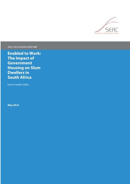
This data is presented in Figure 1 showing the expansion of housing projects over the years
from 1999 to 2009 for areas in Cape Town where housing was built. Figure 7 in the Appendix
shows a broader overview of housing projects for the whole City in 2009.
Figure 1: Housing roll out in Cape Town
1999
Airport
Legend
1996 - 1999
2000 - 2001
2002 - 2004
2005 - 2007
2008 - 2009
2003
Airport
Informal 07
2006
Indian Ocean
2009
Indian Ocean
Airport
Airport
Indian Ocean
Indian Ocean
I aggregated this yearly data into blocks of years corresponding to the time between waves of
the CAPS data to get a measure of how many houses were built, at each location, between each
wave of survey data.
24 There were housing projects placed in the ocean or on the mountain.
25 This dataset was built by Rehana Moorad at the local government department with great accuracy. In some cases
planning department construction blueprints had been used to individually identify housing units in great detail.
12

3.2 Location and Proximity Measures
I used confidential datasets in order to track households as they moved. 26 I used original enumeration
areas maps to locate the original living location of households in the first wave of
the sample, then used household addresses from survey tracking sheets to update household
locations as they moved.
I used ArcGIS maps of the original EAs sampled to map the approximate locations of the
households at the start of the survey. I then used household’s addresses in later waves, transcribed
from the survey documents, to identify households that had changed address. I then
geocoded the new addresses. In this way I tracked households throughout the four waves by
their GPS coordinates. 27 I was then able to generate a range of distance and geographic outcomes
for each household. In each wave of data I calculated the distance from schools, roads,
the city centre, and the distance of move from the original place of living at the basline (if there
was any move at all).
Summary statistics of the migration data are presented in table 2, along with the housing
distance data described in the next section. Roughly 30% of the sample moved at some point
during the survey. 28 The average move distance is small, under 1 km. 29 This data gives an idea
of how far informal households live from the city centre- 26kms on average.
Table 2: Proximity data in wave 3 (2006)
Mean Min Max N Control Treat Diff
City Distance 25.8 4.05 53.3 968 24.7 27.8 3.07***
School Distance 0.48 0.019 3.43 970 0.50 0.45 -0.041
Moved 0.36 0 1 970 0.34 0.40 0.060
Move distance 0.94 0 36.8 970 0.95 0.92 -0.025
Cumulative dist moved 1.53 0 36.8 968 1.37 1.83 0.46
Distance Proj1 0.88 0 16.7 970 1.13 0.41 -0.73***
Distance Proj2 2.41 0 28.6 970 2.82 1.69 -1.13***
Distance Proj3 3.24 0.046 31.2 970 3.60 2.57 -1.04***
Rank Proj1 0.39 0 1 970 0.35 0.48 0.13***
Rank Proj 2 0.11 0 1 970 0.089 0.16 0.068***
3.2.1 Housing Project Distances
Most importantly I was able to generate distances for each household, in each wave, to all of the
government housing projects on which houses had been constructed during the years since the
last survey. For the reasons that become clear in the next section, I focus only on the distance
between housing projects and enumeration areas (EAs) that the household was living in the first
26 These were provided with the help of Jeremy Seekings of the Centre for Social Science Research, University of Cape
Town, and David Lam of Population Studies Center, University of Michigan, after discussions in January 2011.
27 I used Google maps for this. Their batch geoprocessing tools could not always be used because of the considerable
variation in spellings of streets and areas name, especially when in different languages, or in newly developed areas
were street names had not been formalized. Most of these GPS coordinates had to be found by hand.
28 Most of these moves were within the boundaries of the City of Cape Town, but there were a few households that
moved back to rural areas in the Eastern Cape or KwaZulu Nata, some hundreds of kilometers away. For the purposes
of urban relocation analysis, such outliers were excluded from the sample.
29 This may be an underestimate because households that moved further were less likely to be found, and there were
sometimes mistakes with updating address data during the fieldwork.
13

wave. 30 I created dummy variables for EAs that were contained within housing projects, as they
were most likely to be upgraded.
In addition each EA was given a rank (among all other EAs) to each project nearby, such
that each household-project distance pair had a corresponding rank assigned to it. A housing
ranking might not necessarily correspond closely with its distance to a project, if is located in a
densely populated area where many households are competing for treatment.
Table 2 shows these measures, the average distance from the closest housing project, then the
second and third closest. I also show a dummy variable for whether the household lived in the
top 3 closest EAs to the housing project nearest to that household.
4 Empirical Strategy
The paper uses three key strategies for identifying the causal effect of government housing on
household outcomes. Firstly I look at OLS regressions with household fixed effects to estimate
the effect of receiving housing. This gives a basic estimate for the difference-in-difference treatment
effect of housing. Secondly, using a natural experiment that I will explain in detail in
this Section, I instrument for individual selection into treatment (receiving a house) by using
proximity to government housing projects. Thirdly, I use a set of housing projects that were
planned but not built in order to control for selection at the geographic level, by dropping from
the control group those areas that never had projects planned nearby.
Before turning to the formal identifying specifications and assumptions, I describe the natural
experiment that I exploit as part of my identification strategy. In what follows, I use ‘treated’ or
‘treatment households’ to refer to households that received government housing as a result of
the policy.
4.1 Natural Experiment: allocation by proximity
This paper uses the government’s proximity-based allocation policy as a natural experiment.
I focus on the procedures used by the local government in Cape Town. Observations on the
workings of allocation procedures came from numerous meetings and discussions with officials
in the local government in early 2011. 31 Additional policy documents, reports and research
papers on the methods of allocation corroborate this story (Tshangana, 2009; Seekings et al.,
2010; Tissington et al., 2013).
While the official eligibility rules for housing stipulate that households must earn less than
R3500 per month to be eligible for housing, this cut off seems not to be enforced in practice. 32
Once a household has (rightly or wrongly) been deemed eligible, it joins a national housing
waiting list. This list is supposed to work like first-come-first-served queue, but in reality housing
construction at the local level determines the order of delivery, and even within communities
there is evidence that households often jump the queue (Tissington et al., 2013).
30 Importantly, EA centroid locations, instead of their boundaries, were used to calculate distance. This only makes a
noticeable difference for those EAs right next to, or inside projects. I wanted to distinguish EAs that were completely
surrounded by projects from those that simply had part of their boundary overlapping with the boundary of a housing
project.
31 I refer to discussions I had with Paul Whelan (Western Cape Provincial Department of Housing), and Heinrich Lotze
(Head Housing Development Co-ordinator, City of Cape Town Government).
32 Indeed I looked for a discontinuity in the probability of receiving housing at the cut-off in baseline income. While the
probability of receiving housing was definitely lower for very wealthier households, the discontinuity at the eligibility
cut-off was almost non-existent and statistically insignificant. In addition, there are relatively few individuals (only 12%)
in my sample of slum-dwellers who fall above that cut off: the eligibility constraint did not find for them.
14

As a result of the project-by-project nature of the roll out, households were selected into
projects according to catchment areas around the projects. From these areas a number of “source
areas” (particular informal settlements, or communities within settlements) were selected. These
stakeholders were allocated a certain quota of housing units from the project (Tshangana, 2009). 33
That group of communities would establish project committees responsible for allocating housing
to their members, with the one restriction (not always enforced) that all selected candidates
much be on the housing waiting lists. 34
In this way, households that were living close to housing projects that were built between 2002
and 2009 were more likely to be treated than those living further away. It is this relationship
that I exploit as an identification strategy. Of course location of housing projects itself was
not exogenous, making it crucial to understand how housing site locations were selected. The
location of the housing projects was not generally determined by members of communities. In
most cases it was not determined by the government either. The role of private developers in the
housing process meant that land availability and affordability were the main forces determining
construction locations. This meant that housing projects were generally developed in areas
where land was relatively abundant or cheap, or in parcels of undeveloped within the city.
In this way I argue that geographic proximity to new projects was uncorrelated with changes
in household outcomes, except through the channel of improved housing. I will return to this
argument shortly. Firstly, I use a set of the set of distance-from-project measures to predict
selection into treatment, as the first stage of an instrumental variables estimator, discussed in
more detail below.
4.2 Identification
The basic OLS regression of household outcome y it on having government housing T it , including
controls for household observables X it is given by:
y it = α 0 + α i + λ t + X it β + T it τ + δ it + ɛ it (1)
This estimator likely to be biased due to correlation between household unobservables α i and
the housing treatment. In order to account for household unobservables that might be driving
selection into housing, as well as outcomes of interest, I estimate a fixed effects model which
estimates the difference-in-difference impact of receiving government housing:
y it − ȳ i = λ t − ¯λ + (X it − ¯X i )β + (T it − ¯T i )τ + (ɛ it − ¯ɛ i )
ỹ it = ˜λ t + ˜X it β + ˜T it τ + ˜ɛ it (2)
where ỹ it represents the demeaned version of the outcome of interest. The fixed effects estimates
correctly identify the effect of housing under the assumption of common trends. That is,
households that were treated would have had the same changes in y over time had they not been
given the housing, that is: E(δ it |T it = 1) = E(δ it |T it = 0). 35 This requires of course that treated
33 In some cases a certain number of units would be reserved for households outside of the catchment area, usually
communities that had been waiting for a houses for a particularly long time, or had been recently relocated. An example
is the Joe Slovo informal settlement near Langa, which was allocated housing in the N2 Gateway Project due to a fire
that affected that community.
34 Street committees are a common characteristic of most townships in Cape Town and are often those involved in the
management of the communities housing quota allocations. Committee representatives that I met in Cape Town had a
list of their community members who were eligible for housing, which they used to make allocations.
35 For a more detailed discussion of the problem of unobserved time trends in panels, and the resulting bias of
15

households were not effected by different trends or shocks unrelated to housing over time.
4.2.1 Sources of bias
There are a number of reasons to doubt the assumption that treatment is uncorrelated with
individual time shocks. There have been widespread reports of manipulation of the housing
allocation lists, with certain individuals receiving preferential treatment based on political connections
or other means to access housing (even paying bribes) (Seekings et al., 2010; Tissington
et al., 2013). If households who received windfalls or good new jobs were able to leverage their
increased incomes to access housing, this could bias the estimates upwards. 36
On the other hand, it may be the case that housing allocation is more pro-poor such that housing
is allocated by local politicians and communities to households that have the least ability to
improve their own circumstances. Alternatively, households that suffer negative income shocks
might be more likely to be awarded housing. This would bias the estimates of the impact of
housing downwards, as households are less likely to experience increases in their incomes are
most likely to get housing. In the data used in this paper I find that housing is more likely to go
to households that were poorer at baseline.
In addition, the long waiting lists for houses could cause downward selection bias. Many of
households that get treated are likely to be the ones who have remained in informal dwellings
the longest, making them high up the community waiting lists. Those who were able to get out
of poverty and upgrade dwellings on their own are, by definition, off the waiting lists (or at leats
out of my sample of eligible individuals). Thus households would be selected into treatment
due to their relative inability to improve their housing on their own. Finally, measurement error
could be a source of downward bias: the extent of measurement error in the sample could be
substantial, especially in the measurement of incomes, and even in the treatment variable. 37
4.2.2 Instrumental variables estimator
I deal with non-random selection into housing at the individual level through use of an instrumental
variables (IV) estimator. The natural experiment outlined in the previous section allows
me to use distance from housing projects as instrument for selection into housing projects. In
this way I follow McKenzie and Seynabou Sakho (2010), Attanasio and Vera-Hernandez (2004)
and Ravallion and Wodon (2000), who use distance from tax registration offices, community
centres and schooling project, respectively, to control for selection into social programs. 38
Call the relevant distance instrument Z it to estimate a fixed effects-two stage least squares
difference-in-difference estimators see (Bertrand et al., 2004).
36 Given the roll-out of numerous government programs at the same time as the housing project, it is possible that
households that managed to get government housing, also received other benefits simultaneously, which might improve
their economic outcomes
37 Sometimes the interviewed household member might not be able to remember if the household had received the
house from the government. Alternatively households might have moved out of housing after selling it or renting it out,
such that they would mistakenly report not having received government housing.
38 This fits with a larger literature of using geographic instruments. Dinkelman (2011) and Klonner and Nolen (2010)
use terrain data to instrument for the placement of electrification programs and mobile phone antennas, respectively.
These papers follow a methodology pioneered in Duflo and Pande (2007) to evaluate the growth impact of dams.
Similarly Banerjee et al. (2012) uses distances from major roads built across China to evaluate the impact of these roads
on local growth.
16

(FE-2SLS) estimator, given by
ỹ it = ˜λ t + ˜X it β + ˜T it τ + ˜ɛ it (3)
˜T it = ˜λ t + ˜X it π 1 + ˜Z it π 2 + ˜ɛ it (4)
where Equation 4 gives the first stage prediction of the probability of switching to be treated
(receiving a house) from non-treated in time period t. The fitted values for ˜T it are then used as
regressors in Equation 4.2.3. The identifying assumption (exclusion restriction) of this model is
that distance from housing projects is uncorrelated with the change in the outcome of interest:
˜Z it ⊥ ˜δ it + ˜ɛ it . I turn to discuss this assumption in Section 4.4.
In this framework, fixed effects estimation addresses the problem of endogenous time invariant
household unobservables, while endogenous time varying “shocks” to the household are
dealt with through the instrumentation. 39
4.2.3 First stage
It is the distance from multiple housing projects that matters for the probability of receiving
government housing. This presents an econometric challenge since the distance from a single
(closest) housing project is not particularly informative about the probability of treatment. It
is the cumulative effect of numerous housing projects, including the number of houses built
in that project, over the years that predicts selection. After all, if a household was not given
a house by the closest project, it may stand a good chance of winning housing in the next
closest project, especially if it was moved up the waiting list after neighboring households got
houses. Furthermore the number of other households in the neighbourhood of a project will
also influence the probability of receiving housing for a fixed supply of new housing.
In Section A.1 in the Appendix I discuss in more detail some of the challenges arising from
this issue, including a discussion of why alternative measures summarizing the total distance of
households from multiple projects are problematic in terms of the parametric assumptions that
they place on the relationship between distance and selection. In the robustness checks, Section
5.3 I look at the results IV estimates where I simply use a full set of distance measures linear
predictors of treatment in the first stage, and show that the results are consistent with the rest of
the results in the paper, but are estimated imprecisely and with a severe problem of too many
weak instruments.
Instead, I need a flexible estimator to predict selection into treatment that involves multiple
nearby housing projects. I follow Wooldridge (2002) by estimating the probability of treatment
by a non-parametric function G(x, z; ρ) = P(T = 1|x, z), which uses multiple instruments z
and a common coefficient ρ determining the impact of distance on the probability of treatment.
Importantly, the fitted probabilities of the probability of treatment Ĝ cannot be used as regressors
in Equation in the usual 2SLS estimator. These are unlikely to uncorrelated with the error term
as they are in the linear case. 40 Such an estimator will not be consistent. In addition, inference
with this method will produce incorrect standard errors because of the non-linear form of the
regressors and error correction methods would need to be applied.
39 Murtazashvili and Wooldridge (2008) present a more thorough discussion of what I have presented here. They
investigate a more general version of the model I have introduced, using time varying and permanent individual slopes,
and show the conditions required for this model to give consistent estimates of the 2nd stage parameters.
40 The only condition under which such a method would yield an efficient estimator is if data generating process is
perfectly specified by G. We can never really know this and is far too strong an assumption in almost any case (Angrist
and Pischke, 2008).
17

I use an IV estimator adapted from Wooldridge (2002) and applied to the fixed effects case.
Firstly I generate fitted probabilities of treatment Ĝ it for each individual in each period using a
non-linear specification based on a full set of proximity instruments. I then use those predicted
values as an instrument for treatment status T it in the FE-SLS given by Equation 4. In other
words I use a linear projection of T it onto [x, G(x, z; ˆρ)] as the first stage of a 2SLS procedure.
Wooldridge (2002) refers to this as using generated instruments as opposed to generated regressors.
This linear projection will not be correlated with the error term under a valid exclusion
restriction. This follows intuitively from the logic of 2SLS; if the instruments Z are informative
and valid, then G(x, z; ˆρ) will be too.
Wooldridge (2002) shows that in the IV framework, we can ignore the method of estimation of
ρ in the first stage. Inference in the 2SLS with Ĝ it as instruments is consistent, and no standard
error corrections are required. But this non-linear form is more efficient than the linear 2SLS,
and thus more likely to provide valid inference (Newey, 1990).
4.2.4 First Stage Specification
In this section I define the function that determines selection into housing G(x, z; ρ) and the
estimation of ρ (the set of coefficients that capture the effect of distance on receiving housing).
I use maximum likelihood methods to estimate a unique binary outcomes estimator which assume
a latent variable structure for the impact of each distance instrument on the probability of
treatment.
Imagine a household surrounded by a number of housing projets: the aim here is to predict
treatment as a joint function of distance from all of the nearby housing projects as efficiently
as possible. Firstly I use a binary outcomes model to for an expression for the probability of
household i being selected by a particular project a, for each project-household pair. This is
not the same as actually getting housing from that project, since a household cannot receiving
housing twice. I then combine the probability of being selected by each project into an expression
for the joint probability of a household being selected by any housing project. I do not observe
T ia : that is which households received housing from which projects. I observe only T i , the
combined effect of being selected by any project.
Here I use the set of instruments dis ia - the distance between the household and a project built
since the last survey wave. 41 The probability of household being selected housing from a specific
project is given by:
y ⋆ ia = x iβ + dis ia ρ (5)
T ia = 1(y ⋆ > 0)
T ia = 1(x i β + dis ia ρ + v i > 0) (6)
I assume that the error term v takes on the logistic distribution F(y ⋆ ) = Λ(y ⋆ ) = exp(y⋆ )
1+exp(y ⋆ ) such
that
P(T ia = 1) = Λ(x i β + dis ia ρ) (7)
Imagine the case where there are only two projects, and note that a household can receive
41 In the application to the real data we will use a more full set of instruments, all relating to the relationship between
households and individual projects. These are excluded at this point, for ease of exposition.
18

housing from only one project. The likelihood of a household being treated by either project is:
P(T i = 1) = P(T i1 = 1) + P(T i2 = 1) − P(T i1 = 1)P(T i2 = 1)
where P(T ia = 1) is calculated by (7). Notice the adjustment for the fact that a household
cannot be treated more than once. In this framework, the expression P(T ia = 1), given by (7)
has to be interpreted as the project specific contribution to being treated, not the probability of
being treated by that project. For many projects, the probability is most simply expressed as
complement of the probability of being selected by none of the projects:
P(T i = 1) = 1 −
= 1 −
A
∏
a
A
∏
a
(P(T ia = 0)) (8)
Λ(−x i β − dis ia ρ) (9)
This expression, when estimated, gives a single solution to the coefficient ρ, a common effect
of distance for all housing projects, no matter how many different housing projects are used in
the estimation. I use this model to predict the probability of being treatment for a single period,
based on the housing projects that were built in that period.
The problem is complicated further by the use panel data: we’d like efficient estimates for
the probability of receiving housing in each period. Households cannot receiving housing more
than once, so the predicted probability of treatment should decline in a period after a household
had a high predicted probability of treatment, all things equal. We want to derive an expression
for the probability that a household has received housing at point in time up until the specific
period. I development a functional form that conditions the probability of receiving housing in
a particular time period on the probability of having received housing in previous periods.In
the interests of space, this method relegated to the Appendix, Section A.2. There I also develop
a multinominal estimator that predicts, the period in which a household will most likely be
treated.
In addition, I present Monte Carlo simulations using simulations with calibrated parameters
for ρ which gives the effect of proximity on the probability of receiving housing. I find that
the estimator developed here does a good job of recovering the true parameter value for ρ,
even in the presence of considerable noise and individual fixed effects. The average predicted
probabilities of treatment from this model match the rates of treatment in the simulated data.
I am able to estimate the equation given by the 8 and the time (wave) specific probability of
being treated using maximum likelihood techniques. It is to the results of these estimates that I
now turn.
4.3 First Stage Results
I have outlined the key elements on the first stage of my instrumental variables strategy. Taken
together I will estimate a system of equations taking the following form:
ỹ it = ˜λ t + ˜X it β + ˜T it τ + ˜ɛ it (10)
˜T it = ˜δ t + ˜X it δ 1 + ˜Ĝ it π + ṽ it (11)
Ĝ it = G(X it , Z it ; ̂ρ) (12)
19

In this section, I show the results for the estimates of the selection equation (12). The model is
estimated by maximum likelihood, where a single likelihood function describes the probability
of getting housing in each period using all housing projects built during the time period. In
this section show that this method of predicting selection into housing is highly informative and
efficient. I also discuss other interesting predictors of selection into treatment to shed light on
the way in which allocation to housing opportunities happens in practice.
Table 3 shows the estimates for the two different models outlined in the estimation section and
obtained by maximum likelihood programming methods. I show two estimates: “L” denotes the
use of the binary form estimator with a different likelihood function for each time period given
by Equation (13). In this case the dependent variable is T it - whether the household had received
a government house by time period t. By contrast the multinominal “MNL” (described in detail
in Equation (14) in the Appendix) denotes the model with dependent variable TD i - indicating
the period in which the household got the house (or 0 if not at all).
In the estimation I add a range of additional project-household variables to predict treatment
to the basic specification . The distance between the household and the project (ProjectDist ia ), a
dummy variable indicating that the household was actually located within the boundary of the
project (Insitu ia ), and dummy variable indicating that the household’s enumeration area was
ranked among the three closest EAs to the project (Rank ia ). 42 I also include a square term in the
distance from projects, to capture non-linearities in the effect of distance.
Figure 2: Kernel density of predicted treatment for treated and untreated groups
Table 3 shows large and significant impacts of distance from housing on the probability of
receiving housing. Living in an area that was fulling upgraded “in situ” is also a significant
predictor of treatment, as is being one of the closest three households. I discuss some marginal
effects interpretation in the Appendix, Section A.2.1.
The combined effect of the distance has enormous predictive power on the probability of
treatment in the data. I use the coefficients from the estimates in Table 3 to predict treatment
in each time period (Ĝ it ). Using the coefficients from the estimation in Column 1 in Table 3, I
plot the kernel density of predicted treatment by those that actually received housing, and those
42 Such a household might have been upgraded in situ, which was the case for some areas in Cape Town. This dummy
variable indicates that the entire enumeration area (EA) was located within a project, not just that the boundary of the
EA overlapped with a project.
20

Table 3: Maximum likelihood estimation of treatment status
(1) (2) (3) (4) (5) (6) (7)
L L L L MNL MNL MNL
Project Dist -0.499*** -0.515*** -0.396*** -0.672*** -0.534*** -0.514*** -0.561***
(0.100) (0.105) (0.106) (0.142) (0.137) (0.135) (0.164)
Rank 0.687*** 0.735*** 0.662*** 0.350** 0.844*** 0.897*** 0.426*
(0.126) (0.127) (0.130) (0.143) (0.203) (0.202) (0.245)
Project Dist sq .0062*** .0065*** .0044*** .0079*** 0.007*** 0.007*** 0.007***
(.0015) (.0015) (.0017) (.002) (.245) (.244) (.288)
In situ 1.113*** 1.149*** 1.191*** 1.802*** 0.707*** 0.761*** 1.28***
(0.176) (0.177) (0.186) (.196) (.0019) (.0019) (.0023)
Female Head 0.202** 0.166* 0.120 0.312** 0.269*
(0.0895) (0.0910) (0.0957) (0.136) (0.142)
HH Size 0.0859*** 0.0666*** 0.0733*** 0.0219 0.0178
(0.0158) (0.0173) (0.0180) (0.0272) (0.0319)
Sex Ratio -0.610*** -0.637*** -0.544** -0.679** -0.591**
(0.197) (0.201) (0.212) (0.283) (0.295)
Age Ratio 0.153 0.205 0.0658 0.744** 0.667*
(0.224) (0.226) (0.237) (0.325) (0.355)
City Distance 0.04*** 0.05*** 0.04***
(0.00655) (0.00699) (0.0111)
Max Education 0.0267** 0.0319** 0.0132
(0.0126) (0.0134) (0.0194)
From Cape Town -0.515** -0.168
(0.239) (0.344)
Coloured -0.713 -0.713
(0.643) (0.942)
Back yard 0.0492 0.0418
(0.183) (0.277)
Migrant -0.70*** -0.69***
(0.0969) (0.138)
Informal settlement 1.35*** 0.89**
(0.243) (0.348)
Obs 2,694 2,654 2,648 2,648 1,074 1,074 1,074
Time Yes Yes Yes Yes No No No
LL -1430 -1390 -1364 -1284 -838.2 -829.9 -801.9
Notes: Clustered standard errors in parentheses.*** p

that did not, by the final wave of data from 2009. The results show a very clear right shift in the
distribution for treated households.
I note a few other facts about observables that predict access to housing: female headed
households are more likely to get housing, households living further away from the city are more
likely to getting housing even when controlling for distance from projects, perhaps indicating
that higher demand for housing closer to the city leads to housing being allocated differently. 43
Recent migrants (arrived in Cape Town in the last 5 years) are less likely to be treated, perhaps
reflecting the fact that they joined the housing lists later and are there further down the waiting
lists. Households living in communities classified as informal by the city government were also
more likely to get housing: perhaps reflecting that formal slum recognition matters for ensuring
access to services in this context.
4.4 Cancelled Projects
The identification strategy using proximity instruments attempts deals with issues of selection
into treatment based on individual characteristics. It does not necessarily account for nonrandom
selection at the geographic level.
Cancelled Figure and 3: Comparison Complete Projects of 2000-2009 complete and cancelled housing projects
Airport
Indian Ocean
Legend
Cancelled Projects
Complete Projects
The identifying assumption of the IV strategy with fixed effects is that the chosen location
of projects is not correlated with changes in households outcomes over time, except through
the channel of government housing. This assumption may not hold for a number of reasons.
Although all anecdotal reports suggest that communities had very little power in initiating new
housing projects, which were mostly driven by the land demand needs of private construction
companies, it is possible that certain connected individuals were able to lobby effectively for
housing on the part of their communities. These individuals have been successful at lobbying
43 Perhaps ineligible, wealthier households were more likely to jump the queues and get these houses.
22

for other services or employment projects. Further, the government may have prioritized the development
of certain neighborhoods or areas for political reasons, and simultaneously awarded
those areas other social programs.
Figure 4: Predicted probability: comparison with and without incomplete projects
I present a set of robustness checks to show that the results are not driven by larger geographical
variation in treatment: I restrict the estimation to certain areas and townships and find that
the results hold within those sub-samples. Similarly I argue that the results were not driven by
targeting of certain ethnic groups geographically, by restricting the analysis to certain groups
in turn. I also show that receiving government housing did not lead to the receipt of other,
additional government grants. Finally, I argue that housing projects did not stimulate local employment
by creating construction jobs. Construction was always done by external construction
companies that brought in their own permanent labour force to the sites. 44
Figure 5: Predicted probability of treatment in the trimmed sample
Most importantly, I use a natural experiment using housing projects that were planned and
44 In addition, my results show the biggest impact on labour supply of women, who are unlikely to have got jobs on
construction sites.
23

approved but cancelled for bureaucratic reasons. According to discussions with City officials,
this was often due to bureaucratic and budget issues, or problems with the construction companies,
as opposed to something inherent in the local communities in the area. 45 Table 3 shows a
map of the cancelled projects along with completed projects, which gives an idea of the variation
in treatment probabilities induced by project cancellations.
The idea of using cancelled projects is to compare households that lived near planned and
cancelled projects to those that lived near housing projects that were actually built, while excluding
from the sample those households that lived in areas were projects were not even planned.
To do this, I generate a new dataset of distances from housing projects, including the projects
that were cancelled. 46 This new dataset of distances, combined with coefficient estimates from
Table 3, are then used to predict the probability of having been treated had all planned projects
been completed. These predicted probabilities are the counterfactual probabilities of treatment
had all housing been built.
Naturally, this new set of instruments has a smaller average distance to housing- there were
a number of areas that would have been very close to housing projects had their nearby projects
not been cancelled. As a result, the predicted probability of treatment (I call this the “placebo
probabilities”) with the completed projects is considerably higher with the cancelled projects
included. Figure 4 shows the predicted probabilities of treatment with and without cancelled
projects, and a clear right shift for the “placebo probabilities”, and considerably less mass with
probabilities less than 30%.
In order to concentrate on the differences between areas that were near cancelled projects
and those near completed projects, I trim the sample by dropping those far away from both.
That is, I drop individuals with a low probability of treatment with cancelled projects included.
Since many individuals with a relatively high probability of treatment when cancelled projects
are included have a relatively low probability of treatment with only completed projects, the
distribution of the predicted treatment once the sample has been trimmed still has support over
the full range of predicted probabilities. This is illustrated in Figure 5 where all households with
probability of treatment less than 40% are dropped from the sample.
In the main empirical results, I will re-estimate the impacts of receiving housing using
trimmed samples, by iteratively dropping quintiles of the “placebo probabilities” and estimating
both the fixed effects and IV models for those restricted samples.
5 Main Results
In this section I present the main results of the impact of government housing on household
outcomes.
As explained in the empirical strategy, I proceed in three steps: I estimate regular OLS models
with household fixed effects, then use instruments to deal with selection on individual unobservables,
and finally re-estimate both the FE and IV result with a trimmed sample that excludes
areas that were far away from both cancelled and completed projects.
I start by looking at the impacts housing on log of household income.
The income vari-
45 During the time of the study, there were numerous reports of housing projects that were cancelled or put on hold
because the holding companies had become bankrupt
46 Of course, the distance instruments used until now included only distances from completed projects. I carefully
verified that cancelled projects had indeed been cancelled, and that completed projects had indeed been completed, by
using satellite imagery from the time.
24

able comes directly from the CAPS household data. 47 Throughout this section I use the label
“house” to denote this coefficient of interest. Column 1 of Table shows the results from fixed
effects regressions without any controls for changes in household composition, characteristics,
place of living, or other sources of income shows large and significant increases in incomes for
households receiving housing. This effect on total income is about 24%.
Table 4: Effects of government housing on total household income
(1) (2) (3) (4) (5) (6) (7)
FE FE FE IV IV IV IVbal
lginc lginc lginc lginc lginc lginc lginc
house 0.245*** 0.192*** 0.190*** 0.552** 0.617** 0.559* 0.657**
(0.0539) (0.0509) (0.0512) (0.2695) (0.310) (0.313) (0.313)
femalehd -0.188*** -0.188*** -0.172** -0.174** -0.144*
(.0477) (.0480) (.0712) (.0743) (.0798)
hhsize 0.146*** 0.122*** 0.142*** 0.120*** 0.112***
(.0085) (.0126) (.0137) (.0177) (.019)
sexratio -0.174 -0.228* -0.178 -0.231 -0.317*
(0.114) (0.122) (0.140) (0.144) (0.166)
youngratio -0.60*** -0.56*** -0.59*** -0.55*** -0.63***
(0.0921) (0.104) (0.115) (0.129) (0.163)
femadults 0.0353 0.0360 0.0603*
(0.0272) (0.0325) (0.0337)
citydis -0.00705 -0.0128 -0.0212*
(.0079) (.0089) (.0121)
maxedu 0.0209*** 0.0203*** 0.0145*
(.0060) (.0078) (.0084)
maxage 0.00159 0.000842 0.000417
(.0017) (.0024) (.0025)
govgrants 0.0679* 0.0744 0.0899
(0.038) (0.049) (0.059)
Obs 3,590 3,590 3,570 3,572 3,572 3,547 2,526
R 2 0.191 0.284 0.291 0.1828 0.264 0.277 0.272
Groups 1,077 1,077 1,076 1,059 1,059 1,053 661
AvGroup 3.333 3.333 3.318 3.373 3.373 3.368 3.821
McKinnonF . . . 2.62* 5.51*** 4.31*** 2.26***
WeakIVF . . . 70.24 96.98 96.95 91.94
Notes: Clustered standard errors in parentheses.*** p

the estimated effect of housing, but not significantly. The results are similar and still significant
even when controlling for changes in household composition and size. This goes some way to
showing that the effects are not driven by new incomes from new household members.
I then turn to the IV results. As outlined in the estimation section I use the predicted probabilities
from Equation (13) and Table 3 (Column 1) in each time period as instruments in a two
staged least squares estimator. The estimation results of this first stage of the 2SLS is presented
in the Appendix 21.
All IV regressions report the Kleibergen-Paap Wald F statistic for weak instruments. 48 There
is little reason to suspect a problem of weak instruments, given the very high Wald F-statistics
on the test for insignificant instruments in the first stage, reported in the last row of each table.
I find that the IV results estimate large and significant effects of housing on household income.
The coefficients are generally larger than the OLS results, which indicates either correlation
between the probability of treatment and negative income shocks or a problem of measurement
error. 49 As discussed in the conceptual framework, this could be due to individuals in worsening
circumstances (like the aged or recently unemployed), or victims of recent shocks, being assigned
houses by their communities, which leads to downward bias of the treatment effects of housing.
We might have expected them to have done considerably worse without the treatment. Finally,
under the LATE interpretation of my results (see Section 6.5.1) my IV results identify the effects
for households who did not have to move far to get housing, and thus do better than households
that were required to relocate.
Next, I confirm that these results are due to higher average wage earnings for members
of the household. The data on household income used thus far came from a combination of
questions, including a one-shot question on household income when individual earnings were
missing. This may have contained sources of income not related to labour market activities.
I use estimates of the sum of household income from earnings data from household rosters.
However, the data is more often missing for these variables, which yields less precision for the
estimates. Panel A shows the OLS fixed-effects results, Panel B the IV results. The coefficients
on the impacts on household income in logs are significant and similar in magnitude to those in
Table 4.
I also estimate the impact of housing on the per capita income of household members, to rule
out that the effects on incomes were being driven by increases in household size. I find that
receiving housing had a significant impact on the total salary earned by the household, and on
the average earnings per person in the household. In Column 1 I estimate the impact on the
total salary in levels. This is estimated with less precision, but estimates an average impact on
household income of about R350. Average household earnings in the final wave around R2500.
5.1 Cancelled Projects
In this section I use the data on cancelled projects to deal with non-random selection of project
sites. As outlined by the identification strategy, I use the predicted probability of receiving housing
using the projects that were cancelled (I call this the “placebo probability”) in order to drop
48 This is the analogue of Cragg-Donald Wald F statistic, under the assumption of heteroskedastic or serially correlated
errors. Note that in the single endogenous regressor case, such as this one, this statistic is equivalent to standard Wald
test on the first stage coefficient on the single instrument (Baum and Schaffer, 2007).
49 I report post estimation tests of endogeneity, which, in the fixed effect IV setting is the Davidson-MacKinnon F
statistic. This test rejects the null that the IV estimates are the same as the OLS model. See Davidson and MacKinnon
(1993). For the execution of the Fixed Effects Instrumental Variable model with clustered standard errors and 2-Step
GMM I use the stata command xtivreg2, and the dmexogxt post estimation command for exogeneity test of OLS vs XT-IV
estimation (Baum and Stillman, 1999).
26

Table 5: FE and IV Impacts on different earnings measures
(1) (2) (3) (4)
log log log
total salary total salary income/person head’s salary
Panel A: OLS with Fixed Effects Impacts on Different Income Measures
house 348.8* 0.242*** 0.199*** 0.137**
(195.5) (0.0649) (0.0717) (0.0664)
Observations 2,273 1,837 2,438 1,159
R-squared 0.171 0.158 0.236 0.197
Number of hhs 574 574 636 416
Av Group Size 3.960 3.200 3.833 2.786
Panel B: Instrumental Variables Impacts on Different Income Measures
house 568.0 0.520* 0.721** 0.547*
(801.6) (0.304) (0.344) (0.312)
Observations 2,518 1,837 2,438 1,159
R-squared 0.099 0.117 0.185 0.157
Number of hhs 637 574 636 416
Av Group Size 3.953 3.200 3.833 2.786
Weak IV F 79.21 63.30 75.94 44.08
Notes: Clustered standard errors in parentheses. All IV regressions use a non-linear predicted
probability of treatment. house=1 if household reported getting a subsidized house at any point in
the past. Dependent Variable is the log of total household income from wage earnings *** p

Table 6: Impacts on total income with trimming using cancelled projects
(1) (2) (3) (4)
Sample Trimmed % 20 40 60 80
Panel A: OLS with Fixed Effects Impacts on Log Total Income
house 0.163** 0.203*** 0.163** 0.116
(0.0650) (0.0750) (0.0793) (0.0799)
Observations 2,874 2,219 1,507 743
R-squared 0.272 0.271 0.328 0.486
Households 831 625 417 206
Panel B: Instrumental Variables Impacts on Log Total Income
house 0.886** 1.313** 1.409** 0.639
(0.422) (0.571) (0.659) (0.544)
Observations 2,880 2,224 1,510 745
R-squared 0.209 0.123 0.108 0.420
Households 829 623 416 206
Av Group Size 3.474 3.570 3.630 3.617
Weak IV F 53.35 37.73 14.92 15.83
Notes: Clustered standard errors in parentheses. All IV regressions use a nonlinear
predicted probability of treatment. house=1 if household reported getting
a subsidized house at any point in the past. Dependent Variable lginc is the log
of total household income from all sources *** p

Table 7: Impacts on log total salaries with trimming using cancelled projects
(1) (2) (3) (4)
FE FE FE FE
Sample Trimmed % 20 40 60 80
house 0.189** 0.210** 0.191** 0.0751
(0.0741) (0.0797) (0.0867) (0.0910)
Observations 2,167 1,720 1,171 590
R-squared 0.130 0.158 0.199 0.352
Number of personid 719 557 373 184
Av Group Size 3.014 3.088 3.139 3.207
Notes: Clustered standard errors in parentheses.*** p

Paap F statistics for weak instruments are very low: we cannot reject the null of no effect of
the instruments on treatment in the first stage. This problem is improved by the inclusion of
the distance squared as a regressor, but Stock Yogo maximal bias critical values (Stock and
Yogo, 2005) still show that we cannot reject the null of up to 20% bias in IV results. Further,
I have estimated the results using limited information maximum likelihood (LIML) estimation
techniques in which standard errors are correct in the presence of weak instruments: these
estimators inflate the standard errors such that the effects are no longer significant. These results
justify the use of the more precise first stage estimator. 52
6 Mechanisms
In this section I look for mechanisms through which households who received government
housing were able to increase their household incomes. I have documented that these increases
in household income were due to increases in the total wage earnings of individuals in the
household.
In this section, I argue that housing enables household members to leave the home and go out
in search of (more) work, because it alleviates the usual burdens of home production associated
with living in informal housing. I document three main facts about labour outcomes in treated
households. I find that female members of the households are more likely to be employed
after receiving government housing, and that the same results do not apply to male household
members. I find clear evidence that the household earnings from females and males increased
significantly after receiving government housing. For young adult members of the household,
for whom I have more detailed labour data, I find significant impacts of hours worked.
I then look for mechanisms through which labour supply might be restricted by poor housing
conditions. I find that receiving government housing significantly increases feeling of safety.
Receiving housing seems to have moved households further away from the city centre and jobs.
However, these effects are small, compared to anecdotal accounts of how far houses do move in
Cape Town. I also find that improved housing is associated with a number of measures of labour
saving technologies in the home. Finally, I discuss other mechanisms through which housing
might be driving the results, and some limitations of the data to identify these. 53
6.1 Labour Supply
I estimate the effect of government housing on the total number and proportion of women in
the household working in last 7 days before the survey. The results show a significant increase
in female labour supply in households that received government housing. The effects are there
in the fixed effects and the IV regressions.
The impact on the proportion of females employed in the household is not significant in the
fixed effects regression. I find that this is because the treatment effects do not seem to be present
in the early waves of the data- waves 2 and 3. The effects are large and significant however, for
the last wave of the survey. This could be because the effects of moving into new housing take a
52 My non-linear estiamte is considerable more efficient than all other linear first stage estimators, even when the
distance measures are aggregated into a single composite measaure, which improves over the efficiency of the basic
2SLS presented here, but not by much.
53 The data places certain limitations on the mechanisms that can be explored. The CAPS data used in this data focused
on the young adult members of the household, and most of the detailed questions about labour supply and employment
is recorded only for those individuals. Similarly outcomes related to health and small scale enterprises are not well
measured in the data.
30

Table 8: Impacts on male and female labour supply at the extensive margin
(1) (2) (3) (4) (5)
FE FE FD IV IV
num % % num %
employed employed employed employed employed
Panel A: Employment among Female Household Members
subhere 0.102* 0.0285 0.0842* 0.488** 0.325**
(0.0532) (0.0291) (0.0451) (0.237) (0.144)
Observations 2,471 2,471 1,237 2,459 2,458
R-squared 0.032 0.007 0.017 0.087 -0.017
Number of hhs 658 658 654 646 646
Av Group 3.755 3.755 1.891 3.807 3.805
HH Controls Yes Yes Yes Yes Yes
Weak IV F 96.03 86.43
Panel B: Employment among Male Household Members
subhere 0.00256 -0.0200 -0.0497 0.0348 -0.0846
(0.0502) (0.0365) (0.0584) (0.234) (0.171)
Observations 2,471 1,906 947 2,459 1,836
R-squared 0.023 0.014 0.013 0.191 0.059
Number of personid 658 609 589 646 539
Av Group 3.755 3.130 1.608 3.807 3.406
HH Controls Yes Yes Yes Yes Yes
Weak IV F 96.03 40.89
Notes: Clustered standard errors in parentheses.*** p

Table 9: Effect of government housing on hours worked per day (young adults)
(1) (2) (3) (4) (5)
FE FE IV IV IV-Bal
house 0.642** 0.599** 2.289* 2.482* 2.717*
(0.252) (0.256) (1.346) (1.286) (1.480)
HH Chars No Yes No Yes Yes
Obs 1,630 1,605 1,295 1,293 969
Groups 821 813 502 501 356
Av Group 1.985 1.974 2.580 2.581 2.722
Weak IV F 17.20 21.38 9.232
Notes: Clustered standard errors in parentheses.*** p

Table 10: Effect of government housing on earnings of female & male household members
(1) (2) (3) (4)
FE IV FE IV
sum sum average average
earnings earnings earnings earnings
Panel A: Impacts on Earnings of Female Household Members
house 0.200** 0.832* 0.148 0.900*
(0.0899) (0.500) (0.0940) (0.470)
Observations 1,164 1,164 1,139 1,133
R-squared 0.230 0.087 0.115 0.027
Number of hhs 412 412 412 406
Av Group Size 2.825 2.825 2.765 2.791
Weak IV F 36.00 34.05
Panel B: Impacts on Earnings of Male Household Members
house 0.245*** 0.0554 0.255*** 0.113
(0.0888) (0.308) (0.0912) (0.254)
Observations 1,114 1,113 1,098 1,090
R-squared 0.108 0.103 0.096 0.100
Number of hhs 398 398 398 391
Av Group Size 2.799 2.796 2.759 2.788
Weak IV F 35.96 34.21
Notes: Clustered standard errors in parentheses.*** p

Government housing reduces the probability that households use paraffin- a form a fuel
commonly used in informal settlements in South Africa. Many of the devastating fires that
occur in townships in South Africa are attributed to the use of paraffin. There is a negative effect
on the occurrence of fires in the home (although this coefficient is not significant, it was only
measured once in the follow survey rounds) which could be driven by the reduction in paraffin
use.
Table 11: Effects of government housing on living conditions in the home
(1) (2) (3) (4) (5)
FE FE FE FE FE
Panel A: Impact on Household Access to Services
Shack Electricity Toilet Piped Piped In
subhere -0.579*** 0.000640 0.00995 0.102*** 0.242***
(0.0206) (0.0208) (0.0210) (0.0206) (0.0219)
Observations 3,750 3,789 3,789 3,789 3,789
R-squared 0.480 0.041 0.077 0.028 0.157
Number of personid 1,095 1,095 1,095 1,095 1,095
Panel B: Impact on Ownershipo of Household Appliances and Fuel Use
Stove Fridge Microwave Paraffin Fire
subhere 0.0445* 0.0908*** 0.0575** -0.0439* -0.0171
(0.0267) (0.0259) (0.0250) (0.0237) (0.0193)
Observations 3,749 3,749 3,748 2,942 2,949
R-squared 0.149 0.064 0.158 0.002 0.036
Number of hhs 1,095 1,095 1,095 1,095 1,095
Notes: Clustered standard errors in parentheses.*** p

evidence of this in this in Table 12. I find that households that received government housing
were far less likely to report that they felt unsafe in their homes at night.
Table 12: Effects of government housing on feelings of being unsafe at home at night
(1) (2) (3) (4) (5)
FE FE IV IV IVBal
unsafe unsafe unsafe unsafe unsafe
house -0.325*** -0.134** -1.711** -1.169* -0.714*
(0.0548) (0.0643) (0.818) (0.655) (0.411)
HH Chars No Yes No Yes Yes
Observations 1,408 1,376 1,352 1,344 816
R 2 0.039 0.103 -0.631 -0.210 -0.032
Av Group Size 2 1.955 2 2 2
Weak IV F 8.723 11.47 23.92
Notes: Clustered standard errors in parentheses.*** p

I confirm that government housing has moved households slightly further away from the
city, on average. Beneficiary households have not had their situation improved with regards to
distance from the city. Households that receive the government houses move on average 600m
further away from the city during the course of the survey.
Further, this estimate is likely to be an underestimate of the impacts on distance, since for
some households I was not able to geocode their new location, or their location was not updated
by enumerators in the data files. I restrict the sample to households for which a move
is recorded. Here I my point estimates indicate that treated households moved nearly 1.5kms
further away from the city than untreated households. Given that the average distance from the
city is about 22kms in this sample, this is not a huge difference in relative terms. In this sense
the IV results isolate the effects of improved housing without the usual large effect on displacement
that comes with large housing projects of this kind. Government housing had a positive
impact on household labour supply and earnings, in spite of whatever effect housing did have
on distance.
6.5.1 LATE and distance
The results discussed in this paper deserve one important caveat, related to this issue of distance
discussed above. The impact of housing estimated by instrumental variables should be
interpreted as a local average treatment effect (LATE) (Angrist and Imbens, 1994). The instruments
identify the effect of treatment on those household that received housing because of their
proximity to housing. These are known as “compliers” in the framework of Angrist and Imbens
(1994): in the potential outcomes framework they receive government housing if and only if a
housing project is constructed nearby.
The average treatment effect (ATE) is identified by the LATE under the assumption of homogenous
treatment effects (Heckman, 1990). If households that were selected to receive housing
because of their proximity to housing respond differently to treatment than those who receive
housing for different reasons, then this assumption is violated.
This group of compliers is likely to differ from other housing recipients in at least one way.
They are less likely to have moved a significant distance from their original place of living
when receiving housing, precisely because the housing to which they were assigned was close
by to their original place of living. Not all individuals were assigned housing because of their
proximity to housing. A significant number of individuals were able to access housing far away
from their place of living. Among households with predicted probability of receiving housing Ĝ
above the median, 47% received government housing. Among those below the median of value
of Ĝ, 24.3% received housing.
In this way, the estimated impact on distance moved may not fully capture the way in which
households were relocated further away from the city. If individuals who moved further away
from the city centre were likely to suffer worse outcomes because of their distance from jobs and
communities, this could lead to the LATE estimator being an over-estimate of the average treatment
effect. This might explain some of the difference between the OLS fixed-effects estimates
and the IV results presented in this paper.
7 Robustness Checks
In this section I show that the main results on household income, female labour supply and
household wage earnings, are robust to a variety of additional robustness checks.
36

I focus on the validity of the instrumental variables strategy. The validity of the instrumental
variables results would be undermined by challenges to the exclusion restriction: that is that the
location of households in relation to new housing projects is not correlated with the outcomes
of interest except through the channel of government housing.
This assumption could be violated if project placement was driven by community organizing.
I have tried to argue that housing location decisions were more commonly made at levels above
that of the communities. Secondly, I have used the data on planned and cancelled projects to
show that it is the completion of projects, and not just the choice of location, that is driving the
results. Trimming had no effect on the results.
Here I check for robustness by checking that the results are not driven by ambitious households
moving closer to housing projects in order to gain access to housing. Secondly, to mitigate
measurement error in the timing of housing improvements, I estimate a two period first difference
model with just the first and last periods. To ensure that the results are not being driven
by politicians targeting new housing projects to high growth areas or areas where other urban
initiatives were being rolled out, I restrict the analysis to specific areas of the city, and to specific
ethnic groups. Finally, I check for impacts of housing on sources of income other than wage
earnings.
7.1 Opportunistic Relocation
The exclusion restriction would be violated if households were able to move home in order to
access housing. Given that the allocation procedures are well known, highly motivated and mobile
households could be able to move closer to projects that were going ahead before allocation
took place, in order to get a house. This would mean that more motivated households would
also be more likely to be living closer to housing projects.
In practice, this sort of activity is unlikely to have occurred. Most households that receive
government housing have either been on the waiting lists in the local areas in which they receive
housing for many years before they are given this housing. It is unlikely that households would
be able jump the queue after moving to an area so recently. Also all instruments have used
distance from housing in the first wave of the data. Thus if households moved during the period
2002 to 2009 in order to access new housing projects, this change in proximity would not be
reflected in the instruments.
Still, I want to rule out the possibility that the effects were driven by households who had
just moved into new areas in 2002 (the first wave). I drop all households from my sample there
were already treated by wave 2 (2005). This means that everyone who was treated before 2005
is dropped from the sample. I then replicate the main results presented in the paper, with the
instrumental variables and full set of controls, with only households that were treated after 2006.
I find that almost all of the results presented above remain robust to this check. 56 These results
are presented in Table 14, Panel A shows the fixed effects, Panel B the IV estimates. Thus if the
results are driven by successful households relocation decisions, it would have to have been that
they moved to their 2002 location in order to pursue a house that they would only get after 2006.
While housing projects were often subject to delays, it would be unusual if they took longer than
5 years to build.
56 Although standard errors are larger since so many households were treated between 2002 and 2005.
37

Table 14: Replication of the key results without households treated before 2005
(1) (2) (3) (4) (5) (6)
total total female male female % male %
income salary salaries salaries employed employed
Panel A: Fixed Effects Regressions (Multiple Outcomes)
house 0.268*** 0.321*** 0.341*** 0.202* 0.0718* 0.0335
(0.101) (0.103) (0.125) (0.120) (0.0379) (0.0627)
Observations 1,900 1,467 966 918 1,844 1,407
R-squared 0.256 0.127 0.172 0.114 0.036 0.045
Number of hhs 498 489 415 385 494 454
Av Group Size 3.815 3 2.328 2.384 3.733 3.099
Panel A: Instrumental Variables Regressions (Multiple Outcomes)
house 1.401** 1.982** 1.699 -0.154 0.472* 0.298
(0.698) (1.004) (1.127) (0.978) (0.260) (0.310)
Observations 1,900 1,429 858 828 1,835 1,349
R-squared 0.158 -0.120 0.016 0.097 -0.046 0.014
Number of hhs 498 451 307 295 484 396
Av Group Size 3.815 3.169 2.795 2.807 3.791 3.407
Weak IV F 27.57 19.95 13.75 6.726 31.46 23.61
Notes: Clustered standard errors in parentheses.*** p

Table 15: Replication of the key results with a 2-Period first difference estimator
(1) (2) (3) (4) (5) (6)
total total female male female % male %
income salary salaries salaries employed employed
Panel A: Fixed Effects OLS Regressions (Multiple Outcomes)
house 0.285*** 0.265** 0.218 0.285 0.0738* -0.0380
(0.0919) (0.133) (0.187) (0.182) (0.0433) (0.0664)
Observations 1,393 837 404 376 1,360 847
R-squared 0.455 0.266 0.473 0.209 0.050 0.038
Number of hhs 699 419 202 188 680 425
Panel B: Instrumental Variables Regressions (Multiple Outcomes)
house 0.526 0.981** 1.109* 0.413 0.252* -0.113
(0.336) (0.485) (0.600) (0.468) (0.140) (0.167)
Observations 1,388 836 404 376 1,360 850
R-squared 0.448 0.194 0.361 0.206 0.023 0.032
Number of hhs 694 418 202 188 680 425
Av Group Size 2 2 2 2 2 2
Weak IV F 89.97 46.66 22.80 30.57 93.86 47.68
Notes: Clustered standard errors in parentheses.*** p

idence that the effects aren’t driven by geographic selection of project sites. It could be that
projects were targeted to certain parts of the city- parts of the city that had different trajectories
over time. In particular housing could have been targeted towards entire townships, racial
groups, or areas a certain distance from the city, that were exhibiting other changes at the time.
Indeed it does appear that, on average, housing was built in areas further away from the city, in
black areas, and in poorer areas.
Table 16: Average household characteristics by major townships
Gugulethu Khayelitsha Other
N=222 N=608 N=247
Closest Project Distance 0.413 0.144 2.560
Distance to the City 18.57 29.75 21.32
Treated 30% 41% 19.4%
Coloured 7.7% 3.6% 48.8%
Log Income 7.245 7.303 7.598
I divide my sample into three: households living in and around Gugulethu, those living in
Khayelitsha, and those living outside of these two townships. 58 Gugulethu and Khayelitsha are
the two largest townships, or groupings of townships in the city and are where most of the
construction of RDP housing has taken place. Settlements outside of these two townships are
relatively neglected. The mean household characteristics for the different areas are presented in
Table 16. Clearly other informal settlements have less housing construction, are less likely to get
houses, and are more likely to be coloured families. Khayelitsha is further from the center, while
Gugulethu is relatively close.
Table 17 shows the results of regressions of log income and employment on treatment, where
the sample is restricted to various subgroups. For compactness, I report the treatment effects
coefficient for different subgroups in the same columns (both FE and IV). I look in turn at the
three different area in turn, just the poorest half of the sample and just the black sample. Sample
sizes are small in some of the specifications, but the coefficients remain similar in magnitude
to the original results for both FE and IV results for the impacts on household income. This
suggests that the results are not driven by difference across communities, although I find no
evidence of the effect in Gugulethu. 59
In addition I have a great number of households that were living in areas that became housing
projects. These areas were being upgraded in situ (their entire settlement was replaced with new
housing). My use of instruments is less valid for these communities, who may have lobbied for
their particular area to be upgraded. In this way it could be that my instrumental variable results
are picking up the effect of households that were treated because their area was being upgraded
in situ. As a result I drop these households from the sample, leaving only households that were
outside housing developments, and therefore could not have been ensured access to housing. I
find the results are present and just as strong for this group (in panel “Out of Project” in 17).
58 Refer to the map of Cape Town in the Data section. I define Gugulethu rather more broadly than its strict geographical
boundaries; including the townships of Weltevreden Valley, Nyanga, Manenberg and Crossroads Informal
Settlement.
59 This could be cause households in Gugulethu were the household most likely to be moved further away from the
city centre, since it is a relatively dense urban area where there was little space for new housing construction.
40

Table 17: Replication of impacts on Log Income within communities and sub-samples
(1) (2) (3) (4) (5) (6)
FE IV FE IV FE IV
Khayelitsha Gugulethu Other
house 0.262*** 1.243* -0.0150 0.247 0.191*** 0.564*
(0.0844) (0.733) (0.0920) (0.595) (0.0604) (0.314)
Obs 1,471 1,470 730 726 3,582 3,561
R 2 0.276 0.168 0.364 0.357 0.290 0.275
Out of Project Poor Black
house 0.268** 0.988* 0.116* 0.839 0.178*** 0.914**
(0.102) (0.574) (0.0696) (0.562) (0.0641) (0.432)
Obs 1,389 1,377 1,733 1,731 3,015 2,998
R 2 0.328 0.294 0.504 0.451 0.264 0.203
HH Chars Yes Yes Yes Yes Yes Yes
Weak IV F 19.61 13.07 95.24
Notes: Clustered standard errors in parentheses.*** p

I show that the female household members are more likely to be employed in wage paying
labour after receiving government housing. I cannot conclusively ascribe the impact on labour
to any one particular mechanism. I use evidence from time use surveys and qualitative work
on housing conditions to describe the demands on daily life faced by South African households.
These include a lack of to water from some distance away, a lack of security from crime, regular
fires and floods which cause damage to houses, and the use of inefficient and time consuming
cooking and heating technologies.
I provide evidence that government housing alleviates those constraints by improving access
to running water, increasing the probability of ownership of labour saving technologies, reducing
the use of dangerous fuels for lighting and heating, and improving feelings of security in the
home. 61 I also find that housing increases feelings of security in the home which might make it
easier for members to leave the household when they otherwise would have stayed to look after
the home. I argue that these impacts are driving the impacts on female labour supply.
This finding is consistent with the view that living conditions can have an impact on the ability
of females to work (Dinkelman, 2011; Field, 2007). It bolsters the case that informal settlements
can act as a poverty trap to those living in them because of this restriction on labour supply
(Marx et al., 2013).
Government housing in South Africa has had a transformative effect on South Africa’s urban
landscape, with over 25% of the total housing stock estimated to have been built by the government
in the last 20 years. This perceived success has been a cornerstone of the Government’s
electoral platform. Governments elsewhere in the developing world seem to be increasingly
enthusiastic about large scale housing projects of this kind.
Yet projects on this scale are not easy to evaluate. Randomization of such projects is unlikely
to be practically or politically feasible. This paper provides an example of how projects like this
can be evaluated ex post with my unique identification strategy of using the combined effect of
proximity to urban services as instruments for selection into programmes.
This paper highlights the need to take account the effect of urban and housing policy on
the labour outcomes of recipients. Ongoing research is required to fully understand the role of
labour, place of living, neighbourhoods, housing design and finance in determining the efficacy
of urban policy.
61 Data limitations prevent me from investigating the health effects of housing, or looking in more detail at the impact
of housing on time use patterns.
42

References
Angrist, J.D. and Guido W Imbens, “Identification and estimation of local average treatment
effects,” Econometrica, 1994, 62 (2), 467–475.
Angrist, Joshua D and Jorn-Steffen Pischke, Mostly harmless econometrics: an empiricist’s companion,
Princeton Univ Press, 2008.
Ardington, Cally, Anne Case, and Victoria Hosegood, “Labor supply responses to large social
transfers: Longitudinal evidence from South Africa.,” American economic journal. Applied
economics, January 2009, 1 (1), 22–48.
Attanasio, Orazio and Marcos Vera-Hernandez, “Medium- and long run effects of nutrition
and child care: evaluation of a community nursery programme in rural Colombia,” 2004.
Banerjee, Abhijit, Esther Duflo, and Nancy Qian, “On the road: Access to transportation infrastructure
and economic growth in china,” National Bureau of Economic Research, 2012, pp. 1–22.
, Sebastian Galiani, and James Levinsohn, “Why has unemployment risen in the new South
Africa,” IPC Work Paper Series Number 35, 2007.
Barnhardt, Sharon, Erica Field, and Rohini Pande, “Moving to opportunity or isolation? Network
effects of a slum relocation program in India,” mimeo, 2014.
Baum, Christopher F and Mark E. Schaffer, “Enhanced routines for instrumental variables /
generalized method of moments estimation and testing,” Stata Journal, 2007, 7 (4), 465–506.
and Steven Stillman, “{DMEXOGXT}: Stata module to test consistency of {OLS} vs {XT}-{IV}
estimates,” Statistical Software Components, 1999.
Baum-Snow, Nathaniel and Fernando Ferreira, “Causal inference in urban and regional economics,”
Technical Report, National Bureau of Economic Research 2014.
Becker, Gary, “A theory of the allocation of time,” The Economic Journal, 1965, 75 (299), 493–517.
Berniell, M and Carolina Sánchez-Páramo, “Overview of time use data used for the analysis
of gender differences in time use patterns,” Background paper for the World Development Report,
2012.
Bertrand, Marianne, Esther Duflo, and Sendhil Mullainathan, “How much should we trust
differences-in-differences estimates?,” Quarterly Journal of Economics, 2004, 119 (1), 249–275.
Bryan, Gharad, Shyamal Chowdhury, and Ahmed Mushfiq Mobarak, “Underinvestment in a
profitable technology: The case of seasonal migration in Bangladesh,” Econometrica, 2014, 82
(5), 1671–1748.
Budlender, D, N Chobokoane, and Y Mpetsheni, A survey of time use: How South African women
and men spend their time, Statistics South Africa, 2001.
Bundy, Colin, Short-changed: South Africa since Apartheid, Jacana, 2014.
Case, A and A Deaton, “Large cash transfers to the elderly in South Africa,” The Economic
Journal, 1998, 108 (450), 1330–1361.
43

Cattaneo, M.D., S. Galiani, Paul J Gertler, Sebastian Martinez, and R. Titiunik, “Housing,
health, and happiness,” American Economic Journal: Economic Policy, 2009, 1 (1), 75–105.
Centre on Housing Rights and Evictions, “N2 Gateway Project: Housing rights violations as
‘development’ in South Africa,” 2009.
Chance, K, “Housing and evictions at the N2 Gateway Project in Delft,” a report for Abahlali
baseMjondolo, available online at: [http://www. abahlali. org/], 2008.
Charlton, Sarah and C. Kihato, “Reaching the poor? An analysis of the influences on the
evolution of South Africa’s housing programme,” Democracy and Delivery: Urban policy in South
Africa, 2006, pp. 252–282.
City of Cape Town, “Study on the social profile of residents of three selection informal settlements
in Cape Town,” 2005.
Collier, Paul and Anthony J Venables, “Housing and Urbanization in Africa: unleashing a
formal market process,” CSAE Working Paper WPS /2013/01, 2013, 44, 0–18.
Davidson, Russell and James G MacKinnon, Estimation and Inference in Econometrics, Oxford,
UK: Oxford University Press, 1993.
Davis, Mike, Planet of Slums, Verso Books, 2007.
Department of Human Settlements, “National Housing Code,” 2009.
Devoto, Florencia, Esther Duflo, Pascaline Dupas, William Pariente, and Vincent Pons, “Happiness
on tap: piped water adoption in urban Morocco,” Technical Report, National Bureau
of Economic Research 2011.
Dinkelman, Taryn, “The Effects of Rural Electrification on Employment : New Evidence from
South Africa valuable,” American Economic Review, 2011, 101 (7), 3078–3108.
Duflo, Esther, “Grandmothers and Granddaughters: Old-Age Pensions and Intrahousehold Allocation
in South Africa,” The World Bank Economic Review, 2003, 17 (1), 1–25.
, “Women’s empowerment and economic eevelopment,” Journal of Economic Literature, 2012, 50
(4), 1051–1079.
and Rohini Pande, “Dams,” Quarterly Journal of Economics, 2007, 122 (2), 601–646.
, Sebastian Galiani, and Ahmed Mushfiq Mobarak, “Improving access to urban services for
the poor: open issues and a framework for a future research agenda,” J-PAL Urban Services
Review Paper. Cambridge, MA: Abdul Latif Jameel Poverty Action Lab. http://www. povertyactionlab.
org/publication/improving-access-urban-services-poor, 2012.
Field, Erica, “Property rights and investment in urban slums,” Journal of the European Economic
Association, 2005, 3 (2-3), 279–290.
, “Entitled to work: Urban property rights and labor supply in Peru,” Quarterly Journal of
Economics, 2007, 122 (4), 1561–1602.
and Michael Kremer, Impact Evaluation for Slum Upgrading Interventions, World Bank, Poverty
Reduction and Economic Management, Thematic Group on Poverty Analysis, Monitoring and
Impact Evaluation, 2006.
44

Franklin, Simon, “Location, search costs and youth unemployment: A randomized trial of
transport subsidies in Ethiopia,” Working Paper, 2015.
Galiani, Sebastian and Ernesto Schargrodsky, “Property rights for the poor: Effects of land
titling,” Technical Report, Business School Working Paper, Universidad Torcuato Di Tella,
Buenos Aires 2010.
, Paul J Gertler, Ryan Cooper, Sebastian Martinez, Adam Ross, and Raimundo Undurraga,
“Shelter from the storm: Upgrading housing infrastructure in Latin American slums,” IDB
Working Paper, 2014, IDB-WP-528.
Gilbert, Alan G., “Helping the poor through housing subsidies: Lessons from Chile, Columbia
and South Africa,” Habitat International, 2004, 28, 13–40.
, “Free housing for the poor: An effective way to address poverty?,” Habitat International, 2014,
41, 253–261.
Greenwood, Jeremy, Ananth Seshadri, and Mehmet Yorukoglu, “Engines of liberation,” The
Review of Economic Studies, 2005, 72 (1), 109–133.
Gronau, Reuben, “Leisure, Home Production, and Work–the Theory of the Allocation of Time
Revisited,” Journal of Political Economy, 1977, 85 (6), 1099.
Heckman, James, “Varieties of selection bias,” American Economic Review, 1990, 80 (2), 313–318.
Huchzermeyer, Marie, “A legacy of control? The capital subsidy for housing, and informal
settlement intervention in South Africa,” International Journal of Urban and Regional Research,
2003, 27 (3), 591–612.
, “Challenges facing people-driven development in the context of a strong, delivery-oriented
state: Joe Slovo Village, Port Elizabeth,” in “Urban Forum,” Vol. 17 Springer 2006, pp. 25–53.
and Aly Karam, Informal settlements: a perpetual challenge?, Juta and Company Ltd, 2006.
Jacobs, Jane M., The Death and Life of Great American Cities, Vintage books, 1961.
Jalan, Jyotsna and Martin Ravallion, “Does piped water reduce diarrhea for children in rural
India?,” Journal of econometrics, 2003.
Keare, Douglas H and Scott Parris, “Evaluation of Shelter Programs for the Urban Poor Evaluation
of Shelter Programs for the Urban Poor Principal Findings,” 1982.
Klonner, Stefan and Patrick Nolen, “Cell Phones and Rural Labor Markets: Evidence from
South Africa,” Proceedings of the German Development Economics Conference, Hannover
2010 2010.
Lall, Somik V., M. K a Lundberg, and Zmarak Shalizi, “Implications of alternate policies on
welfare of slum dwellers: Evidence from Pune, India,” Journal of Urban Economics, 2008, 63,
56–73.
Lam, David, Jeremy Seekings, and Meredith Sparks, “The Cape Area Panel Study: Overview
and Technical Documentation for Waves 1-2-3,” 2006.
Lipman, Alan, “Apartheid ends, but they’re still put in little boxes, little boxes all the same,” in
“in” November 1998.
45

Marx, Benjamin, Thomas Stoker, and Tavneet Suri, “The economics of slums in the developing
world,” Journal of Economic Perspectives, 2013, 27 (4), 187–210.
McKenzie, David and Y Seynabou Sakho, “Does it pay firms to register for taxes? The impact
of formality on firm profitability,” Journal of Development Economics, 2010, 91 (1), 15–24.
Murtazashvili, I and Jeffrey M Wooldridge, “Fixed effects instrumental variables estimation
in correlated random coefficient panel data models,” Journal of Econometrics, 2008, 142 (1),
539–552.
Newey, W K, “Semiparametric efficiency bounds,” Journal of applied econometrics, 1990, 5 (2),
99–135.
Olsen, Edgar O and Jeffrey E Zabel, “United States housing policy,” in “HandBook of Regional
& Urban Economics” 2014.
Payne, Geoffrey, Alain Durand-Lasserve, Carole Rakodi, Colin Marx, Margot Rubin, and
Selle Ndiaye, “Social and economic impacts of land titling programmes in urban and periurban
areas: International experience and case studies of Senegal and South Africa,” Oslo and
Stockholm: SIDA and Norwegian Ministry of Foreign Affairs, 2008.
Pharoah, Robyn, “Fire Risk in Informal Settlements in Cape Town, South Africa,” Disaster risk
reduction: cases from urban Africa, 2012, p. 105.
Pitt, Mark M., Mark R Rosenzweig, and Nazmul Hassan, “Sharing the Burden of Disease:
Gender, the Household Division of Labor and the Health Effects of Indoor Air Pollution in
Bangladesh and India,” in “Health San Francisco,” Vol. 202 2006.
Ravallion, Martin and Q Wodon, “Does child labour displace schooling? Evidence on behavioural
responses to an enrollment subsidy,” The Economic Journal, 2000, 110 (462), 158–175.
Republic of South Africa, “New Housing Policy and Strategy for South Africa,” Technical
Report 1994.
Rodriques, Elvira, Janet Gie, and Craig Haskins, “Informal Dwelling Count for Cape Town (
1993- 2005 ),” 2006.
Rospabe, Sandrine and Harris Selod, “Does city structure cause unemployment? The case of
Cape Town,” in Haroon Bhorat and Ravi Kanbur, eds., Poverty and Policy in Post-Apartheid
South Africa, HSRC press, 2006, pp. 262–287.
Royston, Lauren, “South Africa: the struggle for access to the city in the Witwatersrand Region,”
Evictions and the right to housing: experience from Canada, Chile, the Dominican Republic, South
Africa, and South Korea, 1998.
, “Security of urban tenure in South Africa: Overview of policy and practice,” Holding their
Ground. Secure Land Tenure for the Urban Poor in Developing Countries, 2002, pp. 165–181.
Sachs, Albie, “The Judicial Enforcement of Socio-Economic Rights: The Grootboom Case,” Current
Legal Problems, 2003, 56 (1), 579–601.
Schwebel, David C., Dehran Swart, Siu Kuen Azor Hui, Jennifer Simpson, and Phumla
Hobeb, “Paraffin-related injury in low-income South African communities: Knowledge, practice
and perceived risk,” Bulletin of the World Health Organization, 2009, 87 (9), 700–706.
46

Seekings, Jeremy, T Jooste, S Muyeba, M Coqui, and M Russell, “The Social Consequences of
‘Mixed’ Neighbourhoods,” CSIR Working Paper, May 2010.
South Africa, “SA govt passes 3-million housing mark,” 2013.
Stock, James H and Motohiro Yogo, “Testing for weak instruments in linear IV regression,
Identification and Inference for Econometric Models: Essays in Honor of Thomas Rothenberg,”
Identification and inference for econometric models: Essays in honor of Thomas Rothenberg, 2005,
pp. 80–108.
Strauss, John, “Does Better Nutrition Raise Farm Productivity?,” Journal of Political Economy,
1986, 94 (2), 297.
and Duncan Thomas, “Health, nutrition, and economic development,” Journal of Economic
Literature, 1998, 36 (2), 766–817.
Tissington, Kate, “A Resource Guide to Housing in South Africa 1994-2010: Legislation, Policy,
Programs and Practice,” 2011.
, N Munshi, G Mirugi-Mukundi, and E Durojaye, “Jumping the Queue: Waiting lists
and other myths: Perceptions and practice around housing demand and allocation in South
Africa,” Technical Report, Socio-economic Rights Institute of South Africa 2013.
Tomlinson, Mary R., “South Africa’s New Housing Policy: An Assessment of the First Two
Years, 1994-96,” International Journal of Urban and Regional Research, 1998, 22 (1), 137–146.
Tshangana, Mbulelo, “Allocation of subsidized housing opportunities to households in the
Western Cape by municipalities,” International Conference, Exhibition and Housing Awards,
Cape Town 2009 April 2009.
UN Habitat, “The Challenge of Slums: Global report on human settlements,” Nairobi, Kenya,
UN: Habitat, 2003.
, State of the World’s Cities 2010/11: Bridging the Urban Divide, Earthscan, 2010.
Vorster, J H and J E Tolken, “Western Cape Occupancy Study,” Technical Report, Department
of Sociology and Social Anthropology, Stellenbosch University 2008.
Werlin, Herbert, “The Slum Upgrading Myth,” Urban Studies, August 1999, 36 (9), 1523–1534.
Wooldridge, Jeffrey M, Econometric Analysis of Cross Section and Panel Data, The MIT Press, 2002.
Zwane, Alix Peterson and Michael Kremer, “What works in fighting diarrheal diseases in developing
countries? A critical review,” World Bank Research Observer, 2007, 22 (1), 1–24.
47

A
Additional information on first stage estimates
This section covers some additional information related to the estimation of the predicted values
for the probability of receiving housing.
I do three things: I explain the rationale for the use of a non-linear predictor of getting
housing, as opposed to other linear estimators, or estimators using a single index of housing
proximity. Secondly, I explain the time-varying multi-nominal version of the estimator outlined,
which explains how I use this framework to predict time varying treatment effects. Thirdly,
I present Monte Carlo estimates that show the reliability of the method to recover the true
parameters of the data generating process it describes.
A.1 Why a non-linear estimator
I estimate the probability of selection into treatment as the joint probability of being selected by
a set of neighboring housing projects. Using only the closest housing project as an instrument
would completely miss the effect of living in an area with a great number of projects, relative to
a house who just has one, very small project nearby. Additionally, the marginal impact of additional
housing projects should diminish as more are built: Consider the possible geographical
scenarios depicted in figure 6 below. We want household 1 to be more likely to be treated than
2 of course, but not three times as likely. After all, we might believe the causal effect of a project
as close as C to be a 50% chance of treatment for household 2 which would lead to considerable
estimation issues for Househould 1 in a linear model. Alternatively, summing distances to all
Figure 6: Hypothetical housing proximity scenarios
A
C
C
B
Household 1 Household 2
A
C
A
C
B
D
Household 3
B
Household 4
D
projects and estimating a single coefficient would severely penalize household 3 to the benefit
of household 1 in the diagram, as 3’s extra project D would increase the sum of distances. However,
placing a different coefficient on the distance from each project, would also be misleadinga
new project’s influence should be diminishing in the probability that a household as already
been selected. For households like 3, project D is unlikely to influence is probability of treatment
at the margin but for households like 4- D could make all the difference.
Trying to incorporate all of these sorts of concerns would involve a great deal of linear restric-
48

tions. Instead I estimate a non-linear model that more closely resembles the real world allocation
process, and avoids the pitfalls of linear models.
I make two main assumptions in the specification of our function form: firstly, that a household’s
probability of selection into a individual housing project is a function of a linear combination
of a number of proximity instruments, as well as household covariates. I also assume
that each project allocates houses independently from the other projects, but that they all do so
with the same catchment area; so that parameter on “distance from a project” is constant across
households, projects and time.
A.2 Time specific predictions
The problem is complicated further when we consider that we have panel data, and need to
estimate a probability of being treated for each time period P(T it = 1) in order to generate a
time varying probability of treatment. This problem is analogous to finding the joint probability
across programs, except that in this case we find the probability across time. Just like one cannot
be treated by two projects at one time, one cannot be treated in more than one time period, and
once you are treated you stay treated for all ensuing periods. Thus the probability of not being
treated at all at time t is simply the product of the probability of not being treated by any projects
built in each time period A t ∈ A, up to and including t. This can be simply rewritten as the sum
of of probabilities across all projects built in the past. In this way, estimation exploits my data on
the timing of housing construction to more accurately predict when households were treated.
t
P(T it = 1) = 1 − ∏ ∏ P(T ia = 0)
j=1 a
A j
A t ,A t−1 ,...
= 1 − ∏
a
P(T ia = 0) (13)
A t ,A t−1 ,...
= 1 − ∏
a
Λ(−x i β − dis ia ρ)
In this functional form (13), the probability for a household at each time is an independent
event. The probability of having the treatment must be monotonically increasing with time (for
each household) as more projects are built. This is the first of two specifications I use to predict
treatment.
A more efficient way to estimate the probability of treatment, which takes into account the
panel nature of the data, is to construct a single likelihood function for each household, which
predicts when the household was treated. Each household is assigned a value for TD, which
takes on 0 if never treated or t = 1, 2, . . . , Y if it received the treatment in period t. These are
mutually exclusive outcomes. We can then estimate a model of multinomial form, in this case
for a Y period model. At each time period we continue to use the form (8) in the calculations.
49

P(TD i = 0) =
4
∏
t=1
A t
∏
a
P(T ia = 0))
A 1
P(TD i = 1) = 1 − ∏ P(T ia = 0)
a
A 2
P(TD i = 2) = (1 − ∏ P(T ia = 0)) ∏ P(T ia = 0)
a a
. . .
A 1
A Y
Y−1 A t
P(TD i = Y) = (1 − ∏ P(T ia = 0)) ∏ ∏ P(T ia = 0) (14)
a t=1 a
Notice how probability of treatment is now conditioned on not having been treated earlier.
For instance, dummy variable TD i = 2 (got treated in period 2) is the probability of not being
selected in period 1 times the probability of being selected in period 2. These dummy variables
and their predicted probabilities must, by definition, must sum to 1.
This dummy indicates the the household actually got the treatment in that period. This is
different to the outcome of interest, which is the probability of having the treatment at a given
time period. This can be backed out by simply summing the predicted dummy variables for
all time periods up to the present. The probability of treatment at a given time period then
simplifies to the same expression given by (13), although the estimation procedure differs. For
instance for could calculate the probability of being treated at time 2 using this framework and
get the expression give by (13) for t = 2:
P(T i2 = 1) = P(TD i = 1) + P(TD i = 2)
A 1
= (1 − ∏ P(T ia = 0)) + (1 − ∏ P(T ia = 0)) ∏ P(T ia = 0)
a
a a
A 1
A 2
A 2
= 1 − ∏ P(T ia = 0) ∏ P(T ia = 0)
a a
2 A t
= 1 − ∏
t
∏
a
P(T ia = 0)
To summarize, I have two non-linear specifications for the probability of being treated at a
given time, equation (13) and equation (14). In both models, probability of being treated in a
certain time period depends on the projects built up until that point. While we would expect (14)
to be the better estimator in the presence of unobserved individual heterogeneity, in the presence
of measurement error, we may get less efficient results because it requires the precise time period
in which the household was treated. The difference between these two types of estimators and
their bias in the presence of unobservables, is explored in the Monte Carlo section below.
A.2.1
Marginal Effects
But first it is useful to have some marginal effects interpretation. This is slightly more complicated
than a standard logit framework, but has an intuitive interpretation. We write down the
probability of being treated at a particular point using the expression (8) and use the properties
A 1
50

of the logistic function, to take the derivative with respect to a particular project b. 62
A
P(T i = 1) = 1 − ∏ Λ(−x i β − dis ia ρ) (15)
a
∂P(T i = 1)
∂dis ib
= 1 −
= −
=
A
∏
a̸=b
A
∏
a
1
1 + exp(x i β + dis ia ρ)
1
1 + exp(x i β + dis ia ρ) · −exp(x i β + dis ib ρ)
(1 + exp(x i β + dis ib ρ)) 2 · ρ
A
1
∏
a 1 + exp(x i β + dis ia ρ) · exp(x i β + dis ib ρ)
1 + exp(x i β + dis ib ρ) · ρ
= P(T i = 0) · P(T ib = 1) · ρ
(16)
In this framework the marginal effects of distance to particular project depend on a household’s
current probability of being treated (negatively) and on the probability of being by the
treated by the project in question (positively). This is consistent with the idea that a new construction
has a relatively bigger effect for a household with few existing projects nearby, and
that the probability of being treated drops off faster the further away a particular project gets.
Using the results from the estimation of the first stage in Section 4.3 and the coefficients in
Column (4): the coefficient on distance is 0.672, on distance squared it is 0.0079. Imagine a
household close to two projects, with characteristics such that the household has a predicted
probability of being selected of 10% for both of the projects. Then imagine that one project (b)
was originally located 1km away but is relocated slightly further away the household. Then
the probability of that household being treated would fall by over 4% for each kilometer that it
moved:
∂P(T i = 1)
∂dis ib
= P(T i = 0) · P(T ib = 1) · (−0.672 + 0.0158 × dis ib )
= (0.9 × 0.9) × 0.1 × (−0.672 + 0.0158 · 1) = −4.16%
A.2.2
Maximum Likelihood Estimation and Monte Carlo Simulations
In this section I estimate the parameters of the models specified in (13) and (14) using simulated
data. Estimation of these models has to be performed using maximum likelihood estimation.
I use the Stata ml code in order to maximize the log likelihood functions derived from the
predicted probability of treatment given by each model, using the Newton-Raphson method.
To perform Monte Carlo tests, I simulate a dataset of N = 1000 observations with 3 time periods
each. Then for each time household-time observation I generate 5 random project distances
(to simulate the construction of houses nearby that household). Each household has a randomly
generated household effect x i that is constant across time and assumed to be unobserved. In
addition, each time period has a random effect on the probability of treatment, common to everyone.
Then, for each project at each time a latent variable is generated as a function of time
62 Of course, taking a partial derivative invokes the ceteris paribus assumption. Strictly speaking, this is not plausible
in my case. Up until now, I have been discussing a set of distances to projects for each household, these projects will
be common to a number of households. So it is hard to imagine the distance from a household to a project changing
without it effecting the distance for other households, which in turn would influence the probability of a household
being treated
51

effects, the household fixed effects and, of course, the distance from the household to the project.
I use a linearly added logistic error term. If this latent variable is greater than zero we consider
a household to be “treated” by that project. A household is treated at that time if it is treated by
any one of the projects, and it remains treated for the ensuing periods.
y ⋆ iat = α + σ xx i + σ λ λ t + ρdis iat + ɛ it
y iat = 1[y ⋆ iat > 0]
A t ,A t−1 ...
y it = 1[
∑
a
y iat > 0]
Where the household characteristics and distance variables are generated in the following way:
x i ∼ N[0, 1], λ t ∼ N[0, 1]
dis iat ∼ U[1, 10]
ɛ it =
exp(η it)
1 + exp(η it ) , η it ∼ U[0, 1]
Having generated simulated values, I recover the parameter of interest, which is ρ, using the
models specified. I estimate three different specifications. The first (L nt ) uses the functional
form (13) but without any attempts to control for time trends. The second (L t ) also uses (13),
but controls for time by specifying time dummies λ t in the latent y ⋆ form. The third (MNL)
is the estimation of (14). I then perform Monte Carlo simulations with 1000 repetitions, for
each model, while varying the magnitude of variance of the unobserved effects. The results of
these simulations, with different “true” values of ρ, are given in table 18. The model performs
Table 18: Results of Monte Carlo Simulations: Estimated value of ρ with different unobserved
fixed and time effects
ρ = −1 ρ = −0.5
L nt L t MNL L nt L t MNL
σx 2 = 0, σλ 2 = 0 -1.013 -1.013 -1.019 -0.507 -0.507 -0.513
(0.148) (0.148) (0.137) (0.078) (0.078) (0.067)
σ 2 x = 1, σ 2 λ = 0 -0.914 -0.915 -0.950 -0.433 -0.433 -0.464
(0.125) (0.125) (0.109) (0.067) (0.067) (0.059)
σ 2 x = 0, σ 2 λ = 1 -0.997 -1.003 -1.007 -0.494 -0.500 -0.503
(0.144) (0.143) (0.143) (0.076) (0.075) (0.076)
σ 2 x = 3, σ 2 λ = 0 -0.742 -0.744 -0.821 -0.330 -0.332 -0.383
(0.099) (0.099) (0.089) (0.061) (0.061) (0.055)
σ 2 x = 0, σ 2 λ = 3 -0.836 -0.904 -0.928 -0.416 -0.481 -0.453
(0.244) (0.175) (0.240) (0.138) (0.082) (0.138)
(N=1000, t=3, R=1000)
very well without any fixed effects or time trends, as expected. The introduction of fixed effect
52

iases the estimates towards zero. The bias can be quite considerable when these fixed effects
are relatively large, as the example with σ 2 x = 3 indicates. The effects are less severe with
the introduction of unobserved time effects, but still biased towards zero. The MNL estimator
performs better when there fixed effects. Importantly, the inclusion of time controls in the L
model does a very good job of recovering the parameters correctly.
53

B
Additional Figures and Tables
54

55
Robben Island
Atlantic Ocean
City Center
Figure 7: Map of Cape Town and its housing projects in 2009
Dunoon
Airport
Delft
Gugulethu
Mfuleni
Khayelitsha
Mitchells Plain
Indian Ocean
Wallacedene
Legend
Housing Projects
Informal Settlements
Strand

Table 19: Household characteristics in first & last waves, by treatment
Wave 1 (2002) Wave 4 (2009)
Control Treatment Diff Control Treatment Diff
From EC 0.712 0.827 0.114 ∗∗∗
(0.0277)
Backyard 0.122 0.0742 -0.0478 ∗
(0.0198)
Coloured 0.187 0.0797 -0.107 ∗∗∗
(0.0228)
Black 0.790 0.915 0.125 ∗∗∗
(0.0238)
Migrant 0.658 0.657 -0.00119
(0.0306)
Shack 1 1 0 0.624 0.188 -0.436 ∗∗∗
(0) (0.0328)
City distance 22.68 25.12 2.434 ∗∗∗ 22.51 25.19 2.681 ∗∗∗
(0.394) (0.436)
Years Ed. head 11.04 11.38 0.341 12.22 12.46 0.238
(0.214) (0.239)
Num. Rooms 3.123 3.259 0.136 3.427 3.828 0.401 ∗∗
(0.0975) (0.122)
HH Size 5.189 5.478 0.289 5.549 6.065 0.516 ∗
(0.149) (0.221)
Female Head 0.488 0.563 0.0751 ∗ 0.533 0.597 0.0649
(0.0321) (0.0361)
Age Head 41.66 42.51 0.854 43.95 46.08 2.129 ∗
(0.758) (0.947)
Young adult employed 0.112 0.0769 -0.0353 0.465 0.460 -0.00472
(0.0193) (0.0360)
% Females Employed 0.442 0.447 0.00439 0.367 0.403 0.0353
(0.0289) (0.0277)
Head Employed 0.691 0.632 -0.0596 ∗ 0.618 0.562 -0.0554
(0.0302) (0.0354)
Health Score 3.858 3.879 0.0214 3.790 4.022 0.233 ∗
(0.0865) (0.0903)
Piped Water 0.130 0.107 -0.0233 0.348 0.534 0.185 ∗∗∗
(0.0211) (0.0351)
Earnings pc 874.9 620.21 -254.75 330.95 400.01 69.06
(254.74) (46.177)
Log Income 7.436 7.218 -0.217 ∗∗∗ 8.194 8.272 0.0784
(0.0606) (0.0635)
Obs 713 364 626 344
56

Table 20: Impact of treatment on household grants and remittances
(1) (2) (3) (4)
FE FE FE FE
hhgrants hhgrants totalsend totalrec
house -0.00495 -0.0245 -484.3 -80.95
(0.0323) (0.0303) (629.7) (197.3)
Observations 3,731 3,723 1,854 1,854
R-squared 0.009 0.140 0.006 0.029
Number of hhs 1,077 1,077 1,062 1,062
HH Chars No Yes Yes Yes
Av Group 3.464 3.457 1.746 1.746
Notes: Clustered standard errors in parentheses.*** p

Table 22: Impacts on young adult labour supply at the extensive margin
(1) (2) (3) (4) (5)
FE FE FD IV IV
num % % num %
employed employed employed employed employed
subhere 0.0338 0.0338 0.0346 0.250** 0.245**
(0.0311) (0.0311) (0.0446) (0.109) (0.112)
Observations 2,648 2,648 1,324 2,623 2,622
R-squared 0.151 0.151 0.307 0.135 0.137
Number of personid 662 662 662 662 662
HH Chars No No No Yes Yes
Av Group 4 4 2 3.962 3.961
Weak IV F . . . 97.08 87.81
Notes: Clustered standard errors in parentheses.*** p

Table 24: Main FE results only among individuals in clusters where many households were
treated
(1) (2) (3) (4) (5) (6)
FE FE FE FE FE FE
lginc lginc lginc ln_hhtotsal ln_hhtotsal ln_hhtotsal
house 0.226*** 0.150** 0.144** 0.193*** 0.181** 0.176**
(0.0609) (0.0588) (0.0582) (0.0656) (0.0722) (0.0719)
femalehead -0.297*** -0.239*** -0.221*** -0.203***
(0.0566) (0.0596) (0.0730) (0.0765)
hhsize 0.133*** 0.143*** 0.0441*** 0.0418***
(0.0102) (0.0110) (0.0124) (0.0136)
citydis -0.0118 -0.00929 -0.0216* -0.0197
(0.0110) (0.0108) (0.0130) (0.0130)
yamom -0.0145 0.0753
(0.0682) (0.0900)
maxhhed 0.0315*** 0.0396***
(0.00718) (0.00911)
sexratio -0.125 -0.184
(0.142) (0.184)
youngratio -0.623*** -0.273*
(0.112) (0.143)
Observations 2,388 2,397 2,393 1,895 1,895 1,892
R-squared 0.216 0.301 0.325 0.129 0.147 0.165
Number of hhs 747 758 758 718 718 718
Av Group Size 3.197 3.162 3.157 2.639 2.639 2.635
Notes: Clustered standard errors in parentheses.*** p

Spatial Economics Research Centre (SERC)
London School of Economics
Houghton Street
London WC2A 2AE
Web: www.spatialeconomics.ac.uk