5128_Ch06_pp320-376

Chapter6
Differential Equations
and Mathematical
Modeling
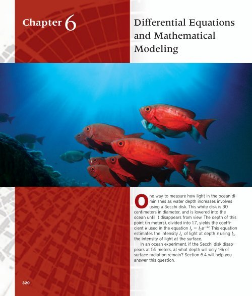
One way to measure how light in the ocean diminishes
as water depth increases involves
using a Secchi disk. This white disk is 30
centimeters in diameter, and is lowered into the
ocean until it disappears from view. The depth of this
point (in meters), divided into 1.7, yields the coefficient
k used in the equation l x l 0 e kx . This equation
estimates the intensity l x of light at depth x using l 0 ,
the intensity of light at the surface.
In an ocean experiment, if the Secchi disk disappears
at 55 meters, at what depth will only 1% of
surface radiation remain? Section 6.4 will help you
answer this question.
320

Section 6.1 Slope Fields and Euler’s Method 321
Chapter 6 Overview
One of the early accomplishments of calculus was predicting the future position of a
planet from its present position and velocity. Today this is just one of a number of occasions
on which we deduce everything we need to know about a function from one of its
known values and its rate of change. From this kind of information, we can tell how long a
sample of radioactive polonium will last; whether, given current trends, a population will
grow or become extinct; and how large major league baseball salaries are likely to be in
the year 2010. In this chapter, we examine the analytic, graphical, and numerical techniques
on which such predictions are based.
6.1
What you’ll learn about
• Differential Equations
• Slope Fields
• Euler’s Method
. . . and why
Differential equations have always
been a prime motivation for the
study of calculus and remain so
to this day.
Slope Fields and Euler’s Method
Differential Equations
We have already seen how the discovery of calculus enabled mathematicians to solve
problems that had befuddled them for centuries because the problems involved moving
objects. Leibniz and Newton were able to model these problems of motion by using equations
involving derivatives—what we call differential equations today, after the notation of
Leibniz. Much energy and creativity has been spent over the years on techniques for solving
such equations, which continue to arise in all areas of applied mathematics.
DEFINITION
Differential Equation
An equation involving a derivative is called a differential equation. The order of a
differential equation is the order of the highest derivative involved in the equation.
EXAMPLE 1
Solving a Differential Equation
Find all functions y that satisfy dydx sec 2 x 2x 5.
SOLUTION
We first encountered this sort of differential equation (called exact because it gives the
derivative exactly) in Chapter 4. The solution can be any antiderivative of sec 2 x 2x 5,
which can be any function of the form y tan x x 2 5x C. That family of functions
is the general solution to the differential equation. Now try Exercise 1.
Notice that we cannot find a unique solution to a differential equation unless we are given
further information. If the general solution to a first-order differential equation is continuous,
the only additional information needed is the value of the function at a single point, called an
initial condition. A differential equation with an initial condition is called an initial value
problem. It has a unique solution, called the particular solution to the differential equation.
EXAMPLE 2
Solving an Initial Value Problem
Find the particular solution to the equation dydx e x 6x 2 whose graph passes
through the point (1, 0).
SOLUTION
The general solution is y e x 2x 3 C. Applying the initial condition, we have
0 e 2 C, from which we conclude that C 2 e. Therefore, the particular
solution is y e x 2x 3 2 e. Now try Exercise 13.

322 Chapter 6 Differential Equations and Mathematical Modeling
An initial condition determines a particular solution by requiring that a solution curve pass
through a given point. If the curve is continuous, this pins down the solution on the entire
domain. If the curve is discontinuous, the initial condition only pins down the continuous
piece of the curve that passes through the given point. In this case, the domain of the solution
must be specified.
EXAMPLE 3
Handling Discontinuity in an Initial Value Problem
Find the particular solution to the equation dydx 2x sec 2 x whose graph passes
through the point (0, 3).
SOLUTION
The general solution is y x 2 tan x C. Applying the initial condition, we have 3
0 0 C, from which we conclude that C 3. Therefore, the particular solution is y
x 2 tan x 3. Since the point (0, 3) only pins down the continuous piece of the general
solution over the interval (p2, p2), we add the domain stipulation p2 x p/2.
Now try Exercise 15.
Sometimes we are unable to find an antiderivative to solve an initial value problem, but
we can still find a solution using the Fundamental Theorem of Calculus.
EXAMPLE 4 Using the Fundamental Theorem to Solve an Initial
Value Problem
Find the solution to the differential equation f (x) e x2 for which f (7) 3.
SOLUTION
This almost seems too simple, but f (x) x
dt 3 has both of the necessary properties!
7 et2
Clearly, f (7) 7
dt 3 0 3 3, and f (x) e
7 et2 x2 by the Fundamental Theorem.
The integral form of the solution in Example 4 might seem less desirable than the explicit
form of the solutions in Examples 2 and 3, but (thanks to modern technology) it
does enable us to find f (x) for any x. For example, f (2) 2
e t2 dt 3
7
fnInt (e^(t 2 ), t, 7,2) 3 1.2317. Now try Exercise 21.
[–2π, 2π] by [–4, 4]
Figure 6.1 A graph of the family of
functions Y 1 sin(x) L 1 , where L 1
{3, 2, 1, 0, 1, 2, 3}. This graph
shows some of the functions that satisfy
the differential equation dydx cos x.
(Example 5)
EXAMPLE 5
Graphing a General Solution
Graph the family of functions that solve the differential equation dy/dx cos x.
SOLUTION
Any function of the form y sin x C solves the differential equation. We cannot
graph them all, but we can graph enough of them to see what a family of solutions
would look like. The command {3, 2, 1, 0, 1, 2, 3,} → L 1 stores seven values of C
in the list L 1 . Figure 6.1 shows the result of graphing the function Y 1 sin(x) L 1 .
Now try Exercises 25—28.
Notice that the graph in Figure 6.1 consists of a family of parallel curves. This should
come as no surprise, since functions of the form sin(x) C are all vertical translations of
the basic sine curve. It might be less obvious that we could have predicted the appearance
of this family of curves from the differential equation itself. Exploration 1 gives you a new
way to look at the solution graph.

Section 6.1 Slope Fields and Euler’s Method 323
EXPLORATION 1
Seeing the Slopes
Figure 6.1 shows the general solution to the exact differential equation dydx cos x.
[–2π, 2π] by [–4, 4]
(a)
1. Since cos x 0 at odd multiples of p2 , we should “see” that dydx 0 at the
odd multiples of p2 in Figure 6.1. Is that true? How can you tell?
2. Algebraically, the y-coordinate does not affect the value of dydx cos x. Why not?
3. Does the graph show that the y-coordinate does not affect the value of dydx?
How can you tell?
4. According to the differential equation dydx cos x, what should be the slope of
the solution curves when x 0? Can you see this in the graph?
5. According to the differential equation dydx cos x, what should be the slope of
the solution curves when x p? Can you see this in the graph?
6. Since cos x is an even function, the slope at any point should be the same as the
slope at its reflection across the y-axis. Is this true? How can you tell?
Exploration 1 suggests the interesting possibility that we could have produced the family
of curves in Figure 6.1 without even solving the differential equation, simply by looking
carefully at slopes. That is exactly the idea behind slope fields.
Slope Fields
[–2π, 2π] by [–4, 4]
(b)
Suppose we want to produce Figure 6.1 without actually solving the differential equation
dydx cos x. Since the differential equation gives the slope at any point (x, y), we can use
that information to draw a small piece of the linearization at that point, which (thanks to
local linearity) approximates the solution curve that passes through that point. Repeating
that process at many points yields an approximation of Figure 6.1 called a slope field. Example
6 shows how this is done.
EXAMPLE 6
Constructing a Slope Field
Construct a slope field for the differential equation dydx cos x.
[–2π, 2π] by [–4, 4]
(c)
SOLUTION
We know that the slope at any point (0, y) will be cos 0 1, so we can start by drawing
tiny segments with slope 1 at several points along the y-axis (Figure 6.2a). Then, since
the slope at any point (p, y) or (p, y) will be 1, we can draw tiny segments with
slope 1 at several points along the vertical lines x p and x p (Figure 6.2b). The
slope at all odd multiples of p2 will be zero, so we draw tiny horizontal segments
along the lines x p2 and x 3p2 (Figure 6.2c). Finally, we add tiny segments
of slope 1 along the lines x 2p (Figure 6.2d).
Now try Exercise 29.
[–2π, 2π] by [–4, 4]
(d)
Figure 6.2 The steps in constructing a
slope field for the differential equation
dydx cos x. (Example 6)
To illustrate how a family of solution curves conforms to a slope field, we superimpose
the solutions in Figure 6.1 on the slope field in Figure 6.2d. The result is shown in Figure 6.3
on the next page.
We could get a smoother-looking slope field by drawing shorter line segments at more
points, but that can get tedious. Happily, the algorithm is simple enough to be programmed
into a graphing calculator. One such program, using a lattice of 150 sample points, produced
in a matter of seconds the graph in Figure 6.4 on the next page.

324 Chapter 6 Differential Equations and Mathematical Modeling
Differential Equation Mode
If your calculator has a differential
equation mode for graphing, it is
intended for graphing slope fields. The
usual “Y” turns into a “dydx ”
screen, and you can enter a function of
x and/or y. The grapher draws a slope
field for the differential equation when
you press the GRAPH button.
[–2π, 2π] by [–4, 4]
Figure 6.3 The graph of the general
solution in Figure 6.1 conforms nicely to
the slope field of the differential equation.
(Example 6)
[–2π, 2π] by [–4, 4]
Figure 6.4 A slope field produced by
a graphing calculator program.
It is also possible to produce slope fields for differential equations that are not of the
form dydx f (x). We will study analytic techniques for solving certain types of these
nonexact differential equations later in this chapter, but you should keep in mind that you
can graph the general solution with a slope field even if you cannot find it analytically.
Can We Solve the Differential
Equation in Example 7?
Although it looks harmless enough,
the differential equation dydx x y
is not easy to solve until you have seen
how it is done. It is an example of a firstorder
linear differential equation, and its
general solution is
y Ce x x 1
(which you can easily check by verifying
that dydx x y). We will defer the
analytic solution of such equations to a
later course.
EXAMPLE 7 Constructing a Slope Field for a Nonexact
Differential Equation
Use a calculator to construct a slope field for the differential equation dydx x y
and sketch a graph of the particular solution that passes through the point (2, 0).
SOLUTION
The calculator produces a graph like the one in Figure 6.5a. Notice the following properties
of the graph, all of them easily predictable from the differential equation:
1. The slopes are zero along the line x y 0.
2. The slopes are 1 along the line x y 1.
3. The slopes get steeper as x increases.
4. The slopes get steeper as y increases.
The particular solution can be found by drawing a smooth curve through the point (2, 0)
that follows the slopes in the slope field, as shown in Figure 6.5b.
[–4.7, 4.7] by [–3.1, 3.1]
(a)
[–4.7, 4.7] by [–3.1, 3.1]
(b)
Figure 6.5 (a) A slope field for the differential equation dy/dx x y, and (b) the
same slope field with the graph of the particular solution through (2, 0) superimposed.
(Example 7)
Now try Exercise 35.

Section 6.1 Slope Fields and Euler’s Method 325
EXAMPLE 8
Matching Slope Fields with Differential Equations
Use slope analysis to match each of the following differential equations with one of the
slope fields (a) through (d). (Do not use your graphing calculator.)
1. d y
x y 2. d y
xy 3. d y
x dx
dx
dx
y 4. d y
y dx
x
(a) (b) (c) (d)
SOLUTION
To match Equation 1, we look for a graph that has zero slope along the line x – y 0.
That is graph (b).
To match Equation 2, we look for a graph that has zero slope along both axes. That is
graph (d).
To match Equation 3, we look for a graph that has horizontal segments when x 0 and
vertical segments when y 0. That is graph (a).
To match Equation 4, we look for a graph that has vertical segments when x 0 and
horizontal segments when y 0. That is graph (c). Now try Exercise 39.
Euler’s Method
In Example 7 we graphed the particular solution to an initial value problem by first producing
a slope field and then finding a smooth curve through the slope field that passed
through the given point. In fact, we could have graphed the particular solution directly, by
starting at the given point and piecing together little line segments to build a continuous
approximation of the curve. This clever application of local linearity to graph a solution
without knowing its equation is called Euler’s Method.
Slope dy/dx
(x, y)
Δx
(x + Δx, y + Δy)
Δy = (dy/dx) Δx
Figure 6.6 How Euler’s Method moves
along the linearization at the point (x, y) to
define a new point (x Δx, y Δy). The
process is then repeated, starting with the
new point.
Euler’s Method For Graphing a Solution to an Initial Value
Problem
1. Begin at the point (x, y) specified by the initial condition. This point will be on
the graph, as required.
2. Use the differential equation to find the slope dydx at the point.
3. Increase x by a small amount Δx. Increase y by a small amount Δy, where
Δy (dy/dx)Δx. This defines a new point (x Δx, y Δy) that lies along the
linearization (Figure 6.6).
4. Using this new point, return to step 2. Repeating the process constructs the graph
to the right of the initial point.
5. To construct the graph moving to the left from the initial point, repeat the process
using negative values for Δx.
We illustrate the method in Example 9.

326 Chapter 6 Differential Equations and Mathematical Modeling
4
3
2
1
0
y
2 2.2 2.4 2.6 2.8 3
Figure 6.7 Euler’s Method is used to
construct an approximate solution to an
initial value problem between x 2 and
x 3. (Example 9)
x
EXAMPLE 9
Applying Euler’s Method
Let f be the function that satisfies the initial value problem in Example 6 (that is,
dydx x y and f (2) 0). Use Euler’s method and increments of Δx 0.2 to
approximate f (3).
SOLUTION
We use Euler’s Method to construct an approximation of the curve from x 2 to x 3,
pasting together five small linearization segments (Figure 6.7). Each segment will extend
from a point (x, y) to a point (x Δx, y Δy), where Δx 0.2 and Δy (dydx)Δx.The
following table shows how we construct each new point from the previous one.
(x, y) dydx x y Δx Δy (dydx)x (x Δx, y Δy)
(2, 0) 2 0.2 0.4 (2.2, 0.4)
(2.2, 0.4) 2.6 0.2 0.52 (2.4, 0.92)
(2.4, 0.92) 3.32 0.2 0.664 (2.6, 1.584)
(2.6, 1.584) 4.184 0.2 0.8368 (2.8, 2.4208)
(2.8, 2.4208) 5.2208 0.2 1.04416 (3, 3.46496)
Euler’s Method leads us to an approximation f (3) 3.46496, which we would more reasonably
report as f (3) 3.465. Now try Exercise 41.
You can see from Figure 6.7 that Euler’s Method leads to an underestimate when the
curve is concave up, just as it will lead to an overestimate when the curve is concave down.
You can also see that the error increases as the distance from the original point increases.
In fact, the true value of f (3) is about 4.155, so the approximation error is about 16.6%.
We could increase the accuracy by taking smaller increments; a reasonable option if we
have a calculator program to do the work. For example, 100 increments of 0.01 give an estimate
of 4.1144, cutting the error to about 1%.
EXAMPLE 10
Moving Backward with Euler’s Method
If dydx 2x y and if y 3 when x 2, use Euler’s Method with five equal steps to
approximate y when x 1.5.
SOLUTION
Starting at x 2, we need five equal steps of Δx 0.1.
(2, 3)
(x, y) dy/dx 2x y Δx Δy (dydx)Δx (x Δx, y Δy)
(2, 3) 1 0.1 0.1 (1.9, 2.9)
(1.9, 2.9) 0.9 0.1 0.09 (1.8, 2.81)
(1.8, 2.81) 0.79 0.1 0.079 (1.7, 2.731)
(1.7, 2.731) 0.669 0.1 0.0669 (1.6, 2.6641)
(1.6, 2.6641) 0.5359 0.1 0.05359 (1.5, 2.61051)
[0, 4] by [0, 6]
Figure 6.8 A grapher program using
Euler’s Method and increments of 0.1
produced this approximation to the solution
curve for the initial value problem in
Example 10. The actual solution curve is
shown in red.
The value at x 1.5 is approximately 2.61. (The actual value is about 2.649, so the
percentage error in this case is about 1.4%.) Now try Exercise 45.
If we program a grapher to do the work of finding the points, Euler’s Method can be
used to graph (approximately) the solution to an initial value problem without actually
solving it. For example, a graphing calculator program starting with the initial value problem
in Example 9 produced the graph in Figure 6.8 using increments of 0.1. The graph of
the actual solution is shown in red. Notice that Euler’s Method does a better job of approximating
the curve when the curve is nearly straight, as should be expected.

Section 6.1 Slope Fields and Euler’s Method 327
Euler’s Method is one example of a numerical method for solving differential equations.
The table of values is the numerical solution. The analysis of error in a numerical
solution and the investigation of methods to reduce it are important, but appropriate for a
more advanced course (which would also describe more accurate numerical methods than
the one shown here).
Quick Review 6.1
In Exercises 1–8, determine whether or not the function y satisfies the
differential equation.
1. d y
y
dx
y e x Yes
2. d y
4y
dx
y e 4x Yes
3. d y
2xy
dx
y x 2 e x No
4. d y
2xy
dx
y e x2 Yes
5. d y
2xy
dx
y e x2 5 No
6. d y
1 dx
y
y 2x
Yes
7. d y
y tan x y sec x Yes
dx
8. d y
y 2 y x 1 No
dx
In Exercises 9–12, find the constant C.
9. y 3x 2 4x C and y 2 when x 1 5
10. y 2sin x 3 cos x C and y 4 when x 0 7
11. y e 2x sec x C and y 5 when x 0 3
12. y tan 1 x ln(2x 1) C and y p when x 1 3p4
Section 6.1 Exercises
In Exercises 1–10, find the general solution to the exact differential
equation.
1. d y
5x 4 sec 2 x
dx
y x 5 tan x C
2. d y
sec x tan x e x
dx
y sec x e x C
3. d y
sin x e x 8x 3
dx
y cos x e x 2x 4 C
4. d y
1 dx
x 1
x2 (x 0) y ln x x 1 C
5. d y
5 x 1
ln 5
dx
x 2
1
y 5 x tan 1 x C
6. d y 1
dx
1 x 1
2 x
y sin 1 x 2x C
7. d y
3t 2 cos(t 3 )
dt
y sin (t 3 ) C
8. d y
(cos t) e sin t
dt
y e sint C
9. d u
(sec 2 x 5 )(5x 4 )
dx
u tan(x 5 ) C
dy
10. 4(sin u) 3 (cos u)
d u
y (sinu) 4 C
In Exercises 11–20, solve the initial value problem explicitly.
11. d y
3 sin x and y 2 when x 0
dx
y 3 cos x 5
12. d y
2e x cos x and y 3 when x 0
dx
y 2e x sin x 1
13. d u
7x 6 3x 2 5 and u 1 when x 1 u x
dx
7 x 3 5x 4
14. d A
10x 9 5x 4 2x 4 and A 6 when x 1
dx
15. d A x 10 x 5 x 2 4x 1
y 1 3
dx
x 2 x 4 12 and y 3 when x 1
16. d y
5 sec 2 x 3 y x 1 x 3 12x 11 (x 0)
x and y 7 when x 0
dx
2
17. d y 5 tan x x 32 7 (0 x < p2)
y 1
dt
1 t 2 2 t ln 2 and y 3 when t 0
y tan 1 t 2 t 2
18. d x
1 dt
t 1
t2 6 and x 0 when t 1
19. d x ln t t 1 6t 7 (t 0)
v
4 sec t tan t e t 6t and v 5 when t 0
dt
20. d v 4 sec t e t 3t 2 (p 2 t p2) (Note that C 0.)
s
t(3t 2) and s 0 when t 1
dt
s t 3 t 2 (Note that C 0.)
In Exercises 21–24, solve the initial value problem using the Fundamental
Theorem. (Your answer will contain a definite integral.)
21. d y
sin (x 2 ) and y 5 when x 1 y x
sin (t
dx
2 )dt 5
1
22. d u
2 s cox
and u 3 when x 0 u x
2s cot
dt 3
dx
0
e cos t dt 9
23. F(x) e cos x and F(2) 9 F(x) x
24. G(s) 3 tan s
and G(0) 4
2
G(s) s
0
3 tan t
dt 4

328 Chapter 6 Differential Equations and Mathematical Modeling
In Exercises 25–28, match the differential equation with the graph of
a family of functions (a)–(d) that solve it. Use slope analysis, not
your graphing calculator.
25. d y
(sin x) 2 Graph (b) 26. d y
(sin x) 3
dx
dx
27. d y
(cos x) 2 Graph (a) 28. d y
(cos x) 3
dx
dx
In Exercises 29–34, construct a slope
field for the differential equation. In
each case, copy the graph at the right
and draw tiny segments through the
twelve lattice points shown in the graph.
Use slope analysis, not your graphing
calculator.
29. d y
x
dx
(a)
(c)
32. d y
2x y
dx
30. d y
y
dx
33. d y
x 2y
dx
Graph (c)
Graph (d)
31. d y
2x y
dx
34. d y
x 2y
dx
In Exercises 35–40, match the differential equation with the appropriate
slope field. Then use the slope field to sketch the graph of the particular
solution through the highlighted point (3, 2). (All slope fields
are shown in the window [6, 6] by [4, 4].)
(a)
(b)
(d)
–1
(b)
2
1
0
–1
y
1
x
35. d y
x
dx
37. d y
x y
dx
39. d y
y dx
x
36. d y
y
dx
38. d y
y x
dx
40. d y
x dx
y
In Exercises 41–44, use Euler’s Method with increments of Δx 0.1
to approximate the value of y when x 1.3.
41. d y
x 1 and y 2 when x 1
dx
2.03
42. d y
y 1 and y 3 when x 1
dx
3.662
43. d y
y x and y 2 when x 1
dx
2.3
44. d y
2x y and y 0 when x 1
dx
0.6
In Exercises 45–48, use Euler’s Method with increments of
Δx 0.1 to approximate the value of y when x 1.7.
45. d y
2 x and y 1 when x 2
dx
0.97
46. d y
1 y and y 0 when x 2
dx
0.271
47. d y
x y and y 2 when x 2
dx
2.031
48. d y
x 2y and y 1 when x 2
dx
1.032
In Exercises 49 and 50, (a) determine which graph shows the solution
of the initial value problem without actually solving the problem.
(b) Writing to Learn Explain how you eliminated two of the
possibilities.
(a) Graph (b)
49. d y 1
, y(0) p dx
1 2 (b) The slope is always positive, so
graphs (a) and (c) can be ruled out.
(a)
x 2
π
2
(e)
y
–1 0 1
x
(b)
π
2
(f)
y
–1 0 1
x
(c)
y
(c)
(d)
π
2
–1 0 1
x

dy
50. x, y1 1 See page 330.
d x
(–1, 1)
0
y
(a)
x
(–1, 1)
0
y
(b)
(–1, 1)
51. Writing to Learn Explain why y x 2 could not be a solution
to the differential equation with slope field shown below.
x
0
y
(c)
x
Section 6.1 Slope Fields and Euler’s Method 329
Since the slopes must be negative reciprocals, g(x) cos x.
56. Perpendicular Slope Fields If the slope fields for the differential
equations dydx sec x and dydx g(x) are perpendicular
(as in Exercise 55), find g(x).
57. Plowing Through a Slope Field The slope field for the differential
equation dy/dx csc x is shown below. Find a function
that will be perpendicular to every line it crosses in the slope
field. (Hint: First find a differential equation that will produce a
perpendicular slope field.) The perpendicular slope field would be
produced by dydx sin x, so y cos x C for any constant C.
[–4.7, 4.7] by [–3.1, 3.1]
52. Writing to Learn Explain why y sin x could not be a
solution to the differential equation with slope field shown
below.
[–4.7, 4.7] by [–3.1, 3.1]
For one thing, there are
positive slopes in the
second quadrant of the
slope field. The graph
of y x 2 has negative
slopes in the second
quadrant.
For one thing, the
slope of y sin x
would be 1 at the
origin, while the slope
field shows a slope of
zero at every point on
the y-axis.
53. Percentage Error Let y f (x) be the solution to the initial
value problem dydx 2x 1 such that f (1) 3. Find the percentage
error if Euler’s Method with Δx 0.1 is used to approximate
f (1.4). See page 330.
54. Percentage Error Let y f (x) be the solution to the initial
value problem dydx 2x 1 such that f (2) 3. Find the percentage
error if Euler’s Method with Δx 0.1 is used to approximate
f (1.6). See page 330.
55. Perpendicular Slope Fields The figure below shows the
slope fields for the differential equations dydx e (xy)/2 and
dy/dx e (yx)/2 superimposed on the same grid. It appears that
the slope lines are perpendicular wherever they intersect. Prove
algebraically that this must be so. See page 330.
x
[–4.7, 4.7] by [–3.1, 3.1]
58. Plowing Through a Slope Field The slope field for the differential
equation dy/dx 1/x is shown below. Find a function
that will be perpendicular to every line it crosses in the slope
field. (Hint: First find a differential equation that will produce a
perpendicular slope field.)
[–4.7, 4.7] by [–3.1, 3.1]
Standardized Test Questions
You should solve the following problems without using a
graphing calculator.
59. True or False Any two solutions to the differential equation
dydx 5 are parallel lines. Justify your answer. True. They are
all lines of the form y 5x C.
60. True or False If f (x) is a solution to dydx 2x, then f 1 (x) is
a solution to dydx 2y. Justify your answer. See page 330.
61. Multiple Choice A slope field for the differential equation
dydx 42 y will show C
(A) a line with slope –1 and y-intercept 42.
(B) a vertical asymptote at x 42.
(C) a horizontal asymptote at y 42.
(D) a family of parabolas opening downward.
(E) a family of parabolas opening to the left.
The perpendicular
slope field would
be produced by
dydx x,
so y 0.5x 2 C
for any constant C.
62. Multiple Choice For which of the following differential equations
will a slope field show nothing but negative slopes in the
fourth quadrant? E
(A) d y
x dx
y
(D) d y
x 3
dx
y2
(B) d y
xy 5
dx
(E) d y y
dx
x 2 3
(C) d y
xy 2 2
dx

330 Chapter 6 Differential Equations and Mathematical Modeling
63. Multiple Choice If dydx 2xy and y 1 when x 0, then
y B
(A) y 2x (B) e x2 (C) x 2 y (D) x 2 y 1 (E) x2 y
2 1
2
64. Multiple Choice Which of the following differential equations
would produce the slope field shown below? A
(A) d y
y x (B) d y
y x
dx
dx
(C) d y
y x (D) d y
y x
dx
dx
(E) d y
y x
dx
Explorations
[–3, 3] by [–1.98, 1.98]
(c) Writing to Learn Explain why y ln x C is
a solution to the differential equation in the domain
, 0 0, . d
ln⏐x⏐ 1 for all x except 0.
d x x
(d) Show that the function
ln x C 1 , x 0
y { ln x C2 , x 0
is a solution to the differential equation for any values of
C 1 and C 2 . d
dy 1 for all x except 0.
x x
Extending the Ideas
67. Second-Order Differential Equations Find the general solution
to each of the following second-order differential equations
by first finding dy/dx and then finding y. The general solution
will have two unknown constants.
(a) d 2y
dx2 12x 4 (b) d 2y
dx2 e x sin x (c) d 2y
dx2 x 3 x 3
68. Second-Order Differential Equations Find the specific solution
to each of the following second-order initial value problems
by first finding dydx and then finding y.
dy
65. Solving Differential Equations Let x d x x
12 .
(a) d 2y
dx2 24x 2 10. When x 1, d y
3 and y 5.
dx
(a) Find a solution to the differential equation in the interval
(b) d 2y
0, that satisfies y1 2. y x 2
2 1 dx2 cos x sin x. When x 0, d y 2x 4 5x 2 5x 3
y
2 and y 0
dx
x 1 2 , x 0
(b) Find a solution to the differential equation in the interval
(c) d 2y
, 0 that satisfies y1 1. y x 2
2 1 dx2 e x x. When x 0, d y cos x sin x x 1
y
0 and y 1.
dx
y e x x 3
x 1
x 3 2 , x 0
6 6
69. Differential Equation Potpourri For each of the following
(c) Show that the following piecewise function is a solution to
differential equations, find at least one particular solution. You
(a) Show that y ln x C is a solution to the differential
55. At every point (x, y), (e (xy) 2 )(e (yx) 2 ) e (xy) 2(yx) 2 e 0 1,
d
equation in the interval 0, . (ln x C) 1 so the slopes are negative reciprocals. The slope lines are therefore
d x
x for x 0
perpendicular.
(b) Show that y ln x C is a solution to the differential 60. False. For example, f (x) x 2 is a solution of dydx 2x, but f 1 (x) x
equation in the interval , 0. d
(ln (x) C) 1 is not a solution of dydx 2y.
Answers:
d x
x for x 0 67. (a) y 2x 3 2x 2 C 1 x C 2 (b) y e x sin x C 1 x C 2
50. (a) Graph (b)
x5
(b) The solution should have positive slope when x is negative, zero slope
(c) y x 1
C1 x C 2 0 2
2
when x is zero and negative slope when x is positive since slope
dydx x. Graphs (a) and (c) don’t show this slope pattern.
69. (a) y x 2
C (b) y x 2
C (c) y Ce x
2
2
53. Euler’s Method gives an estimate f (1.4) 4.32. The solution to the initial (d) y Ce x (e) y Ce x2 2
the differential equation for any values of C 1 and C 2 .
will need to call on past experience with functions you have differentiated.
For a greater challenge, find the general solution.
1 x x 2
C
2 1 , x 0
(a) yx (b) yx (c) yy
y y x 1/x2 , x 0
{ 1 x 1/x
x x (d) y y (e) y xy
C 2 , x 0
22
, x 0
70. Second-Order Potpourri For each of the following secondorder
(d) Choose values for C 1 and C 2 so that the solution in
differential equations, find at least one particular solution.
part (c) agrees with the solutions in parts (a) and (b). C You will need to call on past experience with functions you have
1 3 2 , C 2 1 2
differentiated. For a significantly greater challenge, find the general
solution (which will involve two unknown constants).
(e) Choose values for C 1 and C 2 so that the solution in
part (c) satisfies y2 1 and y2 2. C 1 1 2 , C 2 7 2
(a) yx (b) yx (c) ysin x
66. Solving Differential Equations Let d y
1 dx
x .
(d) yy (e) yy
value problem is f (x) x 2 x 1, from which we get f (1.4) 4.36.
The percentage error is thus (4.36 4.32)/4.36 0.9%.
70. (a) y x 3
C
6 1 x C 2 (b) y x 3
C
6 1 x C 2
54. Euler’s Method gives an estimate f (1.6) 1.92. The solution to the initial
value problem is f (x) x 2 (c) y sin x C
x 1, from which we get f (1.6) 1.96.
1 x C 2 (d) y C 1 e x C 2 e x
The percentage error is thus (1.96 1.92)/1.96 2%.
(e) y C 1 sin x C 2 cos x

Section 6.2 Antidifferentiation by Substitution 331
6.2
What you’ll learn about
• Indefinite Integrals
• Leibniz Notation and
Antiderivatives
• Substitution in Indefinite
Integrals
• Substitution in Definite
Integrals
. . . and why
Antidifferentiation techniques
were historically crucial for applying
the results of calculus.
Antidifferentiation by Substitution
Indefinite Integrals
If y f (x) we can denote the derivative of f by either dydx or f(x). What can we use to
denote the antiderivative of f ? We have seen that the general solution to the differential
equation dy/dx f (x) actually consists of an infinite family of functions of the form
F(x) C, where F(x) f (x). Both the name for this family of functions and the symbol
we use to denote it are closely related to the definite integral because of the Fundamental
Theorem of Calculus.
DEFINITION
Indefinite Integral
The family of all antiderivatives of a function f (x) is the indefinite integral of f
with respect to x and is denoted by f (x)dx.
If F is any function such that F(x) f (x), then f (x)dx F(x) C, where C is an
arbitrary constant, called the constant of integration.
As in Chapter 5, the symbol is an integral sign, the function f is the integrand of the
integral, and x is the variable of integration.
Notice that an indefinite integral is not at all like a definite integral, despite the similarities
in notation and name. A definite integral is a number, the limit of a sequence of Riemann
sums. An indefinite integral is a family of functions having a common derivative. If
the Fundamental Theorem of Calculus had not provided such a dramatic link between antiderivatives
and integration, we would surely be using a different name and symbol for
the general antiderivative today.
EXAMPLE 1
Evaluating an Indefinite Integral
Evaluate (x 2 sin x) dx.
SOLUTION
Evaluating this definite integral is just like solving the differential equation dydx
x 2 sin x. Our past experience with derivatives leads us to conclude that
(x 2 sin x)dx x
3
cos x C
3
(as you can check by differentiating).
Now try Exercise 3.
You have actually been finding antiderivatives since Section 5.3, so Example 1 should
hardly have seemed new. Indeed, each derivative formula in Chapter 3 could be turned
around to yield a corresponding indefinite integral formula. We list some of the most useful
such indefinite integral formulas below. Be sure to familiarize yourself with these before
moving on to the next section, in which function composition becomes an issue. (Incidentally,
it is in anticipation of the next section that we give some of these formulas in
terms of the variable u rather than x.)

332 Chapter 6 Differential Equations and Mathematical Modeling
Properties of Indefinite Integrals
k f (x)dx kf (x) dx
for any constant k
(f (x) g(x)) dx f (x) dx g(x) dx
Power Formulas
1
u n u
du n C when n 1
n 1
u 1 du 1 du ln u C
u
(see Example 2)
Trigonometric Formulas
cos u du sin u C
sec 2 u du tan u C
sec u tan u du sec u C
sin u du cos u C
csc 2 u du cot u C
csc u cot u du csc u C
Exponential and Logarithmic Formulas
e u du e u C
a u du ln
a u a
C
ln u du u ln u u C (See Example 2)
log a u du l n u
du u ln u u
C
ln
a ln a
A Note on Absolute Value
Since the indefinite integral does not
specify a domain, you should always
use the absolute value when finding
1/udu. The function ln u C is only
defined on positive u-intervals, while
the function ln u C is defined on
both the positive and negative intervals
in the domain of 1/u (see Example 2).
EXAMPLE 2
Verifying Antiderivative Formulas
Verify the antiderivative formulas:
(a) u 1 du 1 u du ln u C
SOLUTION
(b) ln u du u ln u u C
We can verify antiderivative formulas by differentiating.
d
d
(a) For u 0, we have (ln u C) (ln u C) 1 d u
d u
u 0 1 u .
d
d
1
For u 0, we have (ln u C) (ln(u) C) (1) 0 1 d u
d u
u
u .
d
Since (lnu C) 1 in either case, ln u C is the general antiderivative of
d u
u
the function 1 on its entire domain.
u
d
(b) (u ln u u C) 1 ln u u d u
( 1 u ) 1 0 ln u 1 1 ln u.
Now try Exercise 11.

Section 6.2 Antidifferentiation by Substitution 333
Leibniz Notation and Antiderivatives
b
The appearance of the differential “dx” in the definite integral a f (x)dx is easily explained
by the fact that it is the limit of a Riemann sum of the form n
f (x k ) Δx (see Section 5.2).
k1
The same “dx” almost seems unnecessary when we use the indefinite integral f (x)dx to
represent the general antiderivative of f, but in fact it is quite useful for dealing with the
effects of the Chain Rule when function composition is involved. Exploration 1 will show
you why this is an important consideration.
EXPLORATION 1 Are f (u) du and f (u) dx the Same Thing?
Let u x 2 and let f (u) u 3 .
1. Find f (u) du as a function of u.
2. Use your answer to question 1 to write f (u) du as a function of x.
3. Show that f (u) x 6 and find f (u) dx as a function of x.
4. Are the answers to questions 2 and 3 the same?
Exploration 1 shows that the notation f (u) is not sufficient to describe an antiderivative
when u is a function of another variable. Just as du/du is different from dudx when
differentiating, f (u) du is different from f (u) dx when antidifferentiating. We will use
this fact to our advantage in the next section, where the importance of “dx” or “du” in the
integral expression will become even more apparent.
EXAMPLE 3
Paying Attention to the Differential
Let f (x) x 3 1 and let u x 2 . Find each of the following antiderivatives in terms of x:
(a)f (x) dx (b) f (u) du (c) f (u) dx
SOLUTION
(a) f (x) dx (x 3 1) dx x 4
4
x C
4
(b) f (u) du (u 3 1) du u u C (x x 2 C x x 2 C
4
4
4
(c) f (u) dx (u 3 1) dx ((x 2 ) 3 1) dx (x 6 1) dx x x C
7
Substitution in Indefinite Integrals
2 ) 4
8
7
Now try Exercise 15.
A change of variables can often turn an unfamiliar integral into one that we can evaluate.
The important point to remember is that it is not sufficient to change an integral of the
form f (x) dx into an integral of the form g(u) dx. The differential matters. A complete
substitution changes the integral f (x) dx into an integral of the form g(u) du.
EXAMPLE 4
Evaluate sin x e cosx dx .
Using Substitution
continued

334 Chapter 6 Differential Equations and Mathematical Modeling
SOLUTION
Let u cos x. Then du/dx sinx, from which we conclude that du sin x dx. We
rewrite the integral and proceed as follows:
sin x ecos x dx (sin x)ecos x dx
e cos x (sin x)dx
e u du
Substitute u for cos x and du for sin x dx.
e u C
e cos x C
Re-substitute cos x for u after antidifferentiating.
Now try Exercise 19.
If you differentiate e cos x C, you will find that a factor of sin x appears when you
apply the Chain Rule. The technique of antidifferentiation by substitution reverses that effect
by absorbing the sin x into the differential du when you change sin x e cos x dx into
e u du . That is why a “u-substitution” always involves a “du-substitution” to convert the
integral into a form ready for antidifferentiation.
EXAMPLE 5
Evaluate x 2 5 2x 3 dx.
SOLUTION
Using Substitution
This integral invites the substitution u 5 2x 3 , du 6x 2 dx.
x2 5 2x 3 dx. (5 2x 3 ) 12 x 2 dx
1 6 (5 2x 3 ) 12 6x 2 dx Set up the substitution with a factor of 6.
1 6 u 12 du
Substitute u for 5 2x 3 and du for 6x 2 dx.
1 6 2 3 u32 C
1 9 (5 2x3 ) 32 C
Re-substitute after antidifferentiating.
Now try Exercise 27.
EXAMPLE 6
Evaluate cot 7x dx.
Using Substitution
SOLUTION
We do not recall a function whose derivative is cot 7x, but a basic trigonometric identity
changes the integrand into a form that invites the substitution u sin 7x, du 7cos 7xdx.
We rewrite the integrand as shown on the next page.

Section 6.2 Antidifferentiation by Substitution 335
cot 7xdx c os
7x
dx
sin
7x
1 7 7co s 7xdx
sin
x
1 7 d u
u
Trigonometric identity
Note that du 7 cos 7x dxwhen u sin 7x
We multiply by 7
1 7, or 1.
Substitute u for 7 sin x and du for 7 cos 7x dx.
1 ln u C
7
Notice the absolute value!
1 ln sin 7x C
7
Re-substitute sin 7x for u after antidifferentiating.
Now try Exercise 29.
EXAMPLE 7 Setting Up a Substitution with a Trigonometric
Identity
Find the indefinite integrals. In each case you can use a trigonometric identity to set up
a substitution.
x
(a) (b) cos
d2 cot 2 3x dx (c) cos 3 x dx
2x
SOLUTION
d
(a) co s
x2x
2 sec 2 2x dx
1 2 sec 2 2x 2dx
1 2 sec 2 u du
Let u 2x and du 2 dx.
1 2 tan u C
1 tan 2x C
2
Re-substitute after antidifferentiating.
(b)cot 2 3x dx (csc 2 3x 1) dx
1 3 (csc 2 3x 1) 3 dx
1 3 (csc 2 u 1) du
Let u 3x and du 3dx.
1 3 (cot u u) C
1 (cot 3x 3x) C
3
1 3 cot 3x x C Re-substitute after antidifferentiation. continued

336 Chapter 6 Differential Equations and Mathematical Modeling
(c)cos 3 x dx (cos 2 x) cos x dx
(1 sin 2 x) cos x dx
(1 u 2 ) du
3
u u C
3
3 x
sin x sin C
3
Let u sin x and du cos x dx.
Re-substitute after antidifferentiating.
Now try Exercise 47.
Substitution in Definite Integrals
Antiderivatives play an important role when we evaluate a definite integral by the Fundamental
Theorem of Calculus, and so, consequently, does substitution. In fact, if we make
full use of our substitution of variables and change the interval of integration to match the
u-substitution in the integrand, we can avoid the “resubstitution” step in the previous four
examples.
EXAMPLE 8 Evaluating a Definite Integral by Substitution
p/3
Evaluate tan x sec 2 x dx.
0
SOLUTION
Let u tan x and du sec 2 x dx.
Note also that u(0) tan 0 0 and u(p/3) tan(p/3) 3.
So
p/3
3
tan x sec 2 x dx u du
0
0
u 2 3
2
0
Substitute u-interval for x-interval.
3 2 0 3 2 Now try Exercise 55.
EXAMPLE 9 That Absolute Value Again
1
x
Evaluate
0 x 2 dx.
4
SOLUTION
Let u x 2 4 and du 2x dx. Then u(0) 0 2 4 4 and u(1) 1 2 4 3.
continued

Section 6.2 Antidifferentiation by Substitution 337
So
1
x
0 x 2 dx 1 1
x
4 2
0 x
22
dx
4
1 3
2 d u
4
u
Substitute u-interval for x-interval.
1 2 ln u 3
4
1 2 (ln 3 ln 4) 1 2 ln 3 4
Notice that ln u would not have existed over the interval of integration [4, 3] . The
absolute value in the antiderivative is important. Now try Exercise 63.
Finally, consider this historical note. The technique of u-substitution derived its importance
from the fact that it was a powerful tool for antidifferentiation. Antidifferentiation
derived its importance from the Fundamental Theorem, which established it as the way to
evaluate definite integrals. Definite integrals derived their importance from real-world
applications. While the applications are no less important today, the fact that the definite
integrals can be easily evaluated by technology has made the world less reliant on antidifferentiation,
and hence less reliant on u-substitution. Consequently, you have seen in this
book only a sampling of the substitution tricks calculus students would have routinely
studied in the past. You may see more of them in a differential equations course.
Quick Review 6.2
(For help, go to Sections 3.6 and 3.9.)
In Exercises 1 and 2, evaluate the definite integral.
5. y x
1. 2
x 4 dx 325 2. 3 2x 2 3 4 4(x 3 2x 2 3) 3 (3x 2 4x)
5
6. y sin
x 1 2 4x 5 8 sin (4x 5) cos (4x 5)
dx 163
0
1
7. y ln cos x tan x
In Exercises 3–10, find dydx.
8. y ln sin x cot x
3. y x
3 t dt 3 x 4. y x
9. y ln sec x tan x sec x
3 t dt 3 x 10. y ln csc x cot x csc x
2
0
Section 6.2 Exercises
In Exercises 1–6, find the indefinite integral.
1. cos x 3x 2 dx 2. x 2 dx x 1 C
sin x x 3 C
3.
t 2 t
1
2 dt t dt
3 3 t 1 C 4.
t
2
1
tan 1 t C
5. 3x 4 2x 3 sec 2 x dx 6. 2e x sec x tan x x dx
(35)x 5 x 2 tan x C
2e x sec x (23)x 32 C
8. (csc u C)(csc u cot u) csc u cot u
In Exercises 7–12, use differentiation to verify the antiderivative
formula.
7. csc 2 u du cot u C 8. csc u cot u csc u C
(cot u C)(csc 2 u) csc 2 u
9. e 2x dx 1 2 e2x C 10. 5 x 1
dx 5 x C
See page 340. ln 5
See page 340.
11. 1
1 u 2 du tan 1 u C 12. 1
1 du sin
u 1 u C
See page 340. 2
See page 340.

338 Chapter 6 Differential Equations and Mathematical Modeling
In Exercises 13–16, verify that f (u) du f (u) dx
13. f (u) u and u x 2 (x 0) See page 340.
14. f (u) u 2 and u x 5 See page 340.
15. f (u) e u and u 7x See page 340.
16. f (u) sin u and u 4x See page 340.
In Exercises 17–24, use the indicated substitution to evaluate the
integral. Confirm your answer by differentiation.
17. sin 3xdx, u 3x 1 cos 3x C
3
18. x cos 2x 2 dx, u 2x 2 1 4 sin (2x2 ) C
19. sec 2x tan 2xdx, u 2x 1 sec 2x C
2
20. 287x 2 3 dx, u 7x 2 (7x 2) 4 C
(1/3) tan 1 (x/3)
dx
21. x
2
, u x C 61 r
3 C
9 3 22. 9r 2 dr
, u 1 r 3
1 r 3
23. ( 1 cos t t sin
2 )2
dt,
2
u 1 cos 2
t
24. 8y 4 4y 2 1 2 y 3 2y dy, u y 4 4y 2 1
2 3 (y 4 4y 2 1) 3 C
In Exercises 25–46, use substitution to evaluate the integral.
1
25. 1
dxx 2 C 1 x
26. sec 2 x 2 dx
2 3 1 cos t
2
3
C
tan (x 2) C
43. 1 3 ln⏐sec (3x)⏐ C 1 3 ln⏐cos (3x)⏐ C
dx
dx
43.
44.
2 co t 3x
5 x 8 5 5x 8 C
45. sec xdx (Hint: Multiply the integrand by
s ec
x tan
x
ln⏐sec x tan x⏐ C
sec
x tan
x
and then use a substitution to integrate the result.)
46. csc xdx (Hint: Multiply the integrand by
c sc
x cot
x
ln⏐csc x cot x⏐ C
csc
x cot
x
and then use a substitution to integrate the result.)
In Exercises 47–52, use the given trigonometric identity to set up a
u-substitution and then evaluate the indefinite integral.
47. sin 3 2xdx, sin 2 2x 1 cos 2 2x co s 3 x
co s x
C
3 2
48. sec 4 xdx, sec 2 x 1 tan 2 x tan x tan C
3
49. 2 sin 2 xdx, cos 2x 2 sin 2 x 1 x sin 2x
C
2
50. 4 cos 2 xdx, cos 2x 1 2 cos 2 x 2x sin 2x C
51. tan 4 xdx, tan 2 x sec 2 x 1 1 3 tan3 x tan x x C
52. (cos 4 x sin 4 x)dx, cos 2x cos 2 x sin 2 x 1 sin 2x C
2
3 x
27. tan x sec 2 xdx 2 3 (tan x)32 C
28. sec
( u p 2 ) tan ( u p 2 ) du sec p 2 C
29. tan(4x 2) dx 30. 3(sin x) 2 dx 3cot x C
In Exercises 53–66, make a u-substitution and integrate from ua
to ub.
53. 3
y 1 dy 14/3 54. 1
r1 r 2 dr 1/3
0
0
55.
4
tan x sec 2 xdx 1/2 56. 1
0
1
5r
4 r 2 2 dr 0
31. cos 3z 4 dz 32. cotx csc 2 xdx
1 2 3 (cot x)3 2 C
sin (3z 4) C
33. ln6 x
dx 1 57.
x 7 (ln x)7 C 34. tan 7 x
sec 2 x
dx
1
10u
du
0 (1 u 3 /2) 2 10/3 58.
cos
x
3 dx 0
4 3 sin x
2 2
1 4 tan8 x
2 C
35. s 13 cos s 43 dx
8 ds 36. sin
2 1 59. 1
6
t 5 2t5t 4 2 dt 60. cos 3 2u sin 2u du 3/4
cot (3x) C
0
0
3x 3
3 23
7
5
4 sin (s 43 8) C
sin
2t
1
6 cos
t
dx
dx
37. dt 38. c os2
2t
1
2 sin
t 2 dt 6 61. 1.504 62.
0 x
0.973
C
2
2 2x 3
2 sin t
(1/2) sec (2t 1) C
2
3p/4
dx
39. ln(ln x) C 40. tan 2 x sec 2 dt
x dx
63.
x
(13) tan
0.693 64.
ln x
1 t
3 x C
cot x dx 0
3
p/4
3
2
x dx
40 dx
41. x
2
42. 8 tan
1
x
2
25
1 x
5 C 65.
x dx
1 x
2
e
0.805 66. x dx
1
0 3 e x 0.954
(12) ln(x 2 1) C
29. (14) ln⏐cos (4x 2)⏐ C or (14) ln⏐sec (4x 2)⏐ C

72. True. Using the substitution u f (x), du f (x)dx, we have
b
f ( x)
dx
f (b)
d u
ln u f (b)
( b)
ln( f (b)) ln( f (a)) ln
a f ( x)
f (a) u
f (a) f
f ( a)
.
Two Routes to the Integral In Exercises 67 and 68, make a
substitution u … (an expression in x), du … . Then
(a) integrate with respect to u from ua to ub.
(b) find an antiderivative with respect to u, replace u by the
expression in x, then evaluate from a to b.
67. 1
x3
(a) 1
dx 2 10 3 2 0.081
0 x 4 9
3
68. 1 cos 3x sin 3xdx (a) 1/2 (b) 1/2
6
Section 6.2 Antidifferentiation by Substitution 339
76. Multiple Choice If the differential equation dy/dx f (x)
leads to the slope field shown below, which of the following
could be f (x) dx? A
(A) sin x C (B) cos x C (C) sin x C
2 x
(D) cos x C (E) sin C
2
(b) 1 2 10 3 2 0.081 Note that dydx tan x
69. Show that
y ln c os
3
cos
x 5
and y(3) 5.
is the solution to the initial value problem
d y
tan x, f 3 5.
dx
(See the discussion following Example 4, Section 5.4.)
70. Show that
y ln
sin
x
s in
2
Note that dydx cot x
6
and y(2) 6.
is the solution to the initial value problem
d y
cot x, f 2 6.
dx
Standardized Test Questions
You should solve the following problems without using
a graphing calculator.
71. True or False By u-substitution, p/4
tan 3 x sec 2 x dx
0
p/4
u 3 du. Justify your answer. See below.
0
72. True or False If f is positive and differentiable on [a, b], then
b
f (x)d
a
f (x
x
)
ln ( b)
f f
( a)
. Justify your answer. See above.
73. Multiple Choice tan x dx D
2 x
(A) tan C
2
(B) ln cot x C
(C) ln cos x C
(D) ln cos x C
(E) ln cot x C
74. Multiple Choice 2 0 e2x dx E
(A) e 4
(B) e 4 1 (C) e 4 2 (D) 2e 4 2 (E) e4 1
2
2
75. Multiple Choice If 5 f (x a) dx 7 where a is a constant,
3
then 5a
f (x) dx
3a B
(A) 7 a (B) 7 (C) 7 a (D) a 7 (E) 7
Explorations
77. Constant of Integration Consider the integral
x 1 dx.
(a) Show that x 1 dx 2 3 x 13/2 C.
(b) Writing to Learn Explain why See page 340.
y 1 x
0
t 1 dt
and y 2 x
3
t 1 dt
are antiderivatives of x 1.
(c) Use a table of values for y 1 y 2 to find the value of C for
which y 1 y 2 C. See page 340.
(d) Writing to Learn Give a convincing argument that
C 3
See page 340.
x 1 dx.
0
78. Group Activity Making Connections Suppose that
f x dx Fx C.
(a) Explain how you can use the derivative of Fx C to
confirm the integration is correct.
(b) Explain how you can use a slope field of f and the graph of
y Fx to support your evaluation of the integral.
(c) Explain how you can use the graphs of y 1 Fx
and y 2 x
f t dt to support your evaluation of the integral.
0
(d) Explain how you can use a table of values for y 1 y 2 ,
y 1 and y 2 defined as in part (c), to support your evaluation of the
integral.
(e) Explain how you can use graphs of f and NDER of Fx to
support your evaluation of the integral.
x
(f) Illustrate parts (a)–(e) for f x .
x
2
1
71. False. The interval of integration should change from [0, p4] to [0, 1],
resulting in a different numerical answer.

340 Chapter 6 Differential Equations and Mathematical Modeling
79. Different Solutions? Consider the integral 2 sin x cos x dx.
(a) Evaluate the integral using the substitution u sin x.
(b) Evaluate the integral using the substitution u cos x.
(c) Writing to Learn Explain why the different-looking
answers in parts (a) and (b) are actually equivalent.
80. Different Solutions? Consider the integral 2 sec 2 x tan x dx.
(a) Evaluate the integral using the substitution u tan x.
(b) Evaluate the integral using the substitution u sec x.
(c) Writing to Learn Explain why the different-looking
answers in parts (a) and (b) are actually equivalent.
Extending the Ideas
81. Trigonometric Substitution Suppose u sin 1 x. Then
cos u 0.
(a) Use the substitution x sin u, dx cos u du to show that
dx
1
x 2 1 du.
(b) Evaluate 1 du to show that 1
dx
x 2 sin 1 x C.
82. Trigonometric Substitution Suppose u tan 1 x.
(a) Use the substitution x tan u, dx sec 2 u du to show that
1
dxx 2 1 du.
(b) Evaluate 1 du to show that 1
dxx 2 tan 1 x C.
83. Trigonometric Substitution Suppose x sin y.
(a) Use the substitution x sin 2 y, dx 2 sin y cos y dy to show
that
p/4
x
dx
2 sin 2 y dy.
x
1
1/2
0
(b) Use the identity given in Exercise 49 to evaluate the definite
integral without a calculator.
84. Trigonometric Substitution Suppose u tan 1 x.
(a) Use the substitution x tan u, dx sec 2 u du to show that
p/3
dx
1
sec u du.
x 2
3
0
(b) Use the hint in Exercise 45 to evaluate the definite integral
without a calculator.
0
0
Answers:
9. 1 2 e2x C 1 2 e2x 2 e 2x
1
10. 5
ln 5
x 1
C 5 x ln 5 5 x
ln 5
11. (tan 1 1
u C) 1 u 2 12. (sin 1 1
u C)
1
u 2
13.f (u) du udu (23)u 3/2 C (2/3)x 3 C
f (u) dx u dx x 2 dx x dx (1/2)x 2 C
14.f (u) du u 2 du (1/3)u 3 C (1/3)x 15 C
f (u) dx u 2 dx x 10 dx (1/11)x 11 C
15.f (u) du e u du e u C e 7x C
f (u) dx e u du e 7x dx (1 7)e 7x C
16.f (u)du sin u du cos u C cos 4x C
f (u) dx sin u dx sin 4 x dx (14) cos 4x C
d
77. (a) d x
2 3 (x 1)3/2 C
x
1
(b) Because dy 1 /dx x 1 and dy 2 /dx x
1
(c) 4 2 3 (d) C y 1 y 2
x 1 dx x
3
x 1 dx 3
x
0
x
0
3
0
x 1 dx
x
x 1 dx
x 1 dx
79. (a) 2 sin x cos x dx 2u du u 2 C sin 2 x C
(b) 2 sin x cos x dx 2u du u 2 C cos 2 x C
(c) Since sin 2 x (cos 2 x) 1, the two answers differ by a constant
(accounted for in the constant of integration).
80. (a) 2 sec 2 x tan x dx 2u du u 2 C tan 2 x C
(b) 2 sec 2 x tan x dx 2u du u 2 C sec 2 x C
(c) Since sec 2 x tan 2 x 1, the two answers differ by a constant
(accounted for in the constant of integration).
dx
81. (a)
1
x cos u d
2 1in
u
s
2 u
cos du
1 du.
co
us 2 u
(Note cos u 0, so cos 2 u ⏐cos u⏐ cos u.)
dx
(b)
1
x 1 du u C 2
sin1 x C
sec 82. (a) 1
dxx 2 2 u du
1 tan2
se c2
u du
u sec
2 1 du
u
(b) 1
dxx 2 1 du u C tan 1 x C
83. (a) 1/2
1/2
x dx
0 1 sin y 2 sin y cos y dy
x
sin1
sin 1 0 1 sin
2 y
p/4
2 sin2 y cos ydy
p/4
2 sin 2 y dy
0 cos
y
0
(b) 1/2 x dx
p/4
2 sin 2 y dy p/4
(1 cos 2y) dy
0 1
x 0
0
[y (1/2)sin 2y] p/4
(p 2)4
0
84. (a) 3 dx
0 1 (3) sec 2 u du
p/3
x 2
tan1 se c2
u du
p/3
sec u du
tan 1 (0) 1n ta
2 u 0 sec
u 0
(b) 3
0
dx
1 x
2
p/3
0
sec u du ln⏐sec u tan u⏐ p3
ln (2 3) ln (1 0) ln (2 3)
0

Section 6.3 Antidifferentiation by Parts 341
6.3
What you’ll learn about
• Product Rule in Integral Form
• Solving for the Unknown Integral
• Tabular Integration
• Inverse Trigonometric and
Logarithmic Functions
. . . and why
The Product Rule relates to derivatives
as the technique of parts
relates to antiderivatives.
Antidifferentiation by Parts
Product Rule in Integral Form
When u and v are differentiable functions of x, the Product Rule for differentiation tells us
that
d
uv u d v
v d u
.
d x dx
dx
Integrating both sides with respect to x and rearranging leads to the integral equation
( u d v
d
) x
( dx d
d
uv) x
( dx v d u
d
) x
dx
uv ( v d u
d
) x
dx.
When this equation is written in the simpler differential notation we obtain the following
formula.
Integration by Parts Formula
u dv uv vdu
This formula expresses one integral, u dv, in terms of a second integral, vdu. With a
proper choice of u and v, the second integral may be easier to evaluate than the first. This is
the reason for the importance of the formula. When faced with an integral that we cannot
handle analytically, we can replace it by one with which we might have more success.
LIPET
If you are wondering what to choose for
u, here is what we usually do. Our first
choice is a natural logarithm (L), if
there is one. If there isn’t, we look for an
inverse trigonometric function (I). If
there isn’t one of these either, look for
a polynomial (P). Barring that, look for
an exponential (E) or a trigonometric
function (T). That’s the preference
order: L IPET.
In general, we want u to be something
that simplifies when differentiated,
and dv to be something that remains
manageable when integrated.
EXAMPLE 1
Evaluate x cos xdx.
SOLUTION
Using Integration by Parts
We use the formula u dv uv vduwith
u x, dv cos xdx.
To complete the formula, we take the differential of u and find the simplest antiderivative
of cos x.
du dx v sin x
Then,
x cos xdx x sin x sin xdx x sin x cos x C.
Now try Exercise 1.
Let’s examine the choices available for u and v in Example 1.

342 Chapter 6 Differential Equations and Mathematical Modeling
EXPLORATION 1
Choosing the Right u and dv
Not every choice of u and dv leads to success in antidifferentiation by parts. There
is always a trade-off when we replace u dv with v du, and we gain nothing if
v du is no easier to find than the integral we started with. Let us look at the other
choices we might have made in Example 1 to find x cos x dx.
1. Apply the parts formula to x cos x dx, letting u 1 and dv x cos x dx.
Analyze the result to explain why the choice of u 1 is never a good one.
2. Apply the parts formula to x cos x dx, letting u x cos x and dv dx. Analyze
the result to explain why this is not a good choice for this integral.
3. Apply the parts formula to x cos x dx, letting u cos x and dv x dx. Analyze
the result to explain why this is not a good choice for this integral.
4. What makes x a good choice for u and cos x dx a good choice for dv?
The goal of integration by parts is to go from an integral u dvthat we don’t see how to
evaluate to an integral vduthat we can evaluate. Keep in mind that integration by parts
does not always work.
Sometimes we have to use integration by parts more than once to evaluate an integral.
EXAMPLE 2
Evaluate x 2 e x dx.
SOLUTION
Repeated Use of Integration by Parts
With u x 2 , dv e x dx, du 2xdx,and v e x , we have
x 2 e x dx x 2 e x 2xe x dx.
The new integral is less complicated than the original because the exponent on x is
reduced by one. To evaluate the integral on the right, we integrate by parts again with
u x, dv e x dx. Then du dx, v e x , and
Hence,
xe x dx xe x e x dx xe x e x C.
x 2 e x dx x 2 e x 2xe x dx
x 2 e x 2xe x 2e x C.
The technique of Example 2 works for any integral x n e x dx in which n is a positive
integer, because differentiating x n will eventually lead to zero and integrating e x is easy.
We will say more on this later in this section when we discuss tabular integration.
Now try Exercise 5.
EXAMPLE 3
Solving an Initial Value Problem
Solve the differential equation dy/dx x ln(x) subject to the initial condition y 1
when x 1. Confirm the solution graphically by showing that it conforms to the slope
field.
continued

Section 6.3 Antidifferentiation by Parts 343
SOLUTION
We find the antiderivative of x ln(x) by using parts. It is usually a better idea to differentiate
ln(x) than to antidifferentiate it (do you see why?), so we let u ln(x) and dv xdx.
y x ln(x) dx
2
x 2
x 2
ln(x)
x 2
2
2
1 x dx
ln(x)
2
x dx
Using the initial condition,
2
x
2
ln(x) x C
4
2
1 1 2 ln(1) 1 4 C
3 4 0 C
Thus
C 3 4 .
2
y x
2
ln(x) x 3 4 4 .
2
Figure 6.9 shows a graph of this function superimposed on a slope field for
dy/dx x ln(x), to which it conforms nicely. Now try Exercise 11.
[0, 3] by [–1.5, 1.5]
Figure 6.9 The solution to the initial
value problem in Example 3 conforms
nicely to a slope field of the differential
equation. (Example 3)
Solving for the Unknown Integral
Integrals like the one in the next example occur in electrical engineering. Their evaluation
requires two integrations by parts, followed by solving for the unknown integral.
EXAMPLE 4
Evaluate e x cos xdx.
SOLUTION
Solving for the Unknown Integral
Let u e x , dv cos xdx. Then du e x dx, v sin x, and
e x cos xdx e x sin x e x sin xdx.
The second integral is like the first, except it has sin x in place of cos x. To evaluate it,
we use integration by parts with
u e x , dv sin xdx, v cos x, du e x dx.
Then
e x cos xdx e x sin x ( e x cos x cos xe dx)
x
e x sin x e x cos x e x cos xdx.
continued

344 Chapter 6 Differential Equations and Mathematical Modeling
The unknown integral now appears on both sides of the equation. Adding the integral to
both sides gives
2e x cos xdx e x sin x e x cos x C.
Dividing by 2 and renaming the constant of integration gives
e x e
cos xdx x sin x e x cos x
C.
2
Now try Exercise 17.
When making repeated use of integration by parts in circumstances like Example 4,
once a choice for u and dv is made, it is usually not a good idea to switch choices in the second
stage of the problem. Doing so will result in undoing the work. For example, if we had
switched to the substitution u sin x, dv e x dx in the second integration, we would have
obtained
e x cos xdx e x sin x ( e x sin x e x cos xdx)
undoing the first integration by parts.
Tabular Integration
e x cos xdx,
We have seen that integrals of the form f xgxdx, in which f can be differentiated repeatedly
to become zero and g can be integrated repeatedly without difficulty, are natural
candidates for integration by parts. However, if many repetitions are required, the calculations
can be cumbersome. In situations like this, there is a way to organize the calculations
that saves a great deal of work. It is tabular integration, as shown in Examples 5 and 6.
EXAMPLE 5 Using Tabular Integration
Evaluate x 2 e x dx.
SOLUTION
With f x x 2 and gx e x , we list:
f x and its derivatives
gx and its integrals
x 2 e x
2x e x
2 e x
0 e x
We combine the products of the functions connected by the arrows according to the
operation signs above the arrows to obtain
x 2 e x dx x 2 e x 2xe x 2e x C.
Compare this with the result in Example 2. Now try Exercise 21.

Section 6.3 Antidifferentiation by Parts 345
EXAMPLE 6
Evaluate x 3 sin xdx.
SOLUTION
Using Tabular Integration
With f x x 3 and gx sin x, we list:
f x and its derivatives
gx and its integrals
x 3 sin x
3x 2 cos x
6x sin x
6 cos x
0 sin x
Again we combine the products of the functions connected by the arrows according to
the operation signs above the arrows to obtain
x 3 sin xdxx 3 cos x 3x 2 sin x 6x cos x 6 sin x C.
Now try Exercise 23.
Inverse Trigonometric and Logarithmic Functions
The method of parts is only useful when the integrand can be written as a product of two
functions (u and dv). In fact, any integrand f (x) dx satisfies that requirement, since we can
let u f (x) and dv dx. There are not many antiderivatives of the form f (x) dx that you
would want to find by parts, but there are some, most notably the antiderivatives of logarithmic
and inverse trigonometric functions.
EXAMPLE 7 Antidifferentiating ln x
Find ln x dx.
SOLUTION
If we want to use parts, we have little choice but to let u ln x and dv dx.
ln x dx (ln x)(x) (x)
1 x
dx
udv uv vdu
x ln x 1 dx
x ln x x C
EXAMPLE 8
Antidifferentiating sin 1 x
Find the solution to the differential equation dy/dx sin 1 x if the graph of the solution
passes through the point (0, 0).
SOLUTION
We find sin 1 x dx, letting u sin 1 x, dv dx.
continued

346 Chapter 6 Differential Equations and Mathematical Modeling
1
sin 1 x dx (sin 1 x)(x) (x) 1 x dx 2
udv uv vdu
x sin 1 x x dx
1
x 2
x sin 1 x 1 2 2x
dx
1
Set up u-substitution.
x2
x sin 1 x 1 2 u 1/2 du
Let u 1 x 2 , du = 2x dx.
x sin 1 x u 1/2 C
x sin 1 x 1 x 2 C
Re-substitute.
[–1, 1] by [–0.5, 0.5]
Figure 6.10 The solution to the initial
value problem in Example 8 conforms
nicely to the slope field of the differential
equation. (Example 8)
Applying the initial condition y 0 when x 0, we conclude that the particular solution
is y x sin 1 x 1 x 2 1.
A graph of y x sin 1 x 1 x 2 1 conforms nicely to the slope field for
dy/dx sin 1 x, as shown in Figure 6.10.
9. y 1 2 x2 cos x 3
Quick Review 6.3 (For help, go to Sections 3.8 and 3.9.)
In Exercises 1–4, find dydx.
3e2x
2e 8. Solve the differential equation dy/dx e 2 x . y 1 2x ln (3x 1)
2 e2x C
1. y x 3 2x 3 cos 2x 3x 2 sin 2x 3x 1
sin 2x 2. y e 2 x ln 3x 1
9. Solve the initial value problem dy/dx x sin x, y0 2.
3. y tan 1 2x 4. y sin 1 1
x 3
1 1
24x 2
(x 3) 2
10. Use differentiation to confirm the integration formula
In Exercises 5 and 6, solve for x in terms of y.
5. y tan 1 3x x 1 3 tan y 6. y cos1 x 1 e x sin xdx 1 x cos y 1
e
2 x sin x cos x.
d
7. Find the area under the arch of the curve y sin x from x 0
d x
to x 1. 2
1 2 ex (sin x cos x) ex sin x
p
Section 6.3 Exercises
In Exercises 1–10, find the indefinite integral.
1. x sin xdx 2. x e x dx xe x e x C
x cos x sin x C
3. 3t e 2t dt 3 2 te2t 3 4 e2t C 4. 2t cos(3t) dt
5. x 2 cos xdx 6. x 2 e x dx
x 2 sin x 2x cos x 2 sin x C
7. 3x 2 e 2x dx 8. x 2 x
cos 2 dx
2 3 t sin (3t) 2 cos (3t) C
9
x 2 e x 2xe x 2e x C
9. y ln ydy y 2
ln y y 2
C 10. t 2 ln t dt t 3
ln t t 3
C
2 4
3 9
7. 3 2 x2 e 2x 3 2 xe2x 3 4 e2x C 8. x 2x2 sin 2
x
8x cos 2
x
16 sin 2 C
In Exercises 11–16, solve the initial value problem. Confirm your answer
by checking that it conforms to the slope field of the differential
equation.
11. d y
(x 2) sin x and y 2 when x 0
dx
12. d y
2xe x and y 3 when x 0
dx
13. d u
x sec 2 x and u 1 when x 0
dx
dz
14. x 3 ln x and z 5 when x 1
d x
15. d y
xx 1 and y 2 when x 1
dx
16. d y
2xx 2 and y 0 when x 1
dx

x
19. e (2 sin 2x cos 2x) C 20. e (2 cos 2x sin 2x) C
5
5
In Exercises 17–20, use parts and solve for the unknown integral.
17. e x sin xdx 18. e x cos x dx
e x
(sin x cos x) C
2
e x
(sin x cos x) C
2
19. e x cos 2xdx 20. e x sin 2x dx
In Exercises 21–24, use tabular integration to find the antiderivative.
21. x 4 e x dx 22. x 2 5xe x dx
23. x 3 e 2 x dx See page 348. 24. x 3 cos 2x dx
In Exercises 25–28, evaluate the integral analytically. Support your
answer using NINT.
2
25. 0
27. 3
2
2
x 2 sin 2xdx
26. x 3 cos 2xdx
p 2
1 0
8 2 0.734
e 2 x cos 3xdx 28. 2
3 4 3 p2
1.101
16
e 2 x sin 2xdx
See page 348.
3 See page 348.
In Exercises 29–32, solve the differential equation.
29. d y
x
dx
2 e 4 x See page 348. 30. d y
x
dx
2 ln x See page 348.
dy
31. u sec d u
1 dy
u, u 1 32. u sec u tan u
See page 348. d u See page 348.
33. Finding Area Find the area of the region enclosed by the
x-axis and the curve y x sin x for
(a) 0 x p, p (b) p x 2p, 3p (c) 0 x 2p. 4p
34. Finding Area Find the area of the region enclosed by the
y-axis and the curves y x 2 and y x 2 x 1e x . 0.726
35. Average Value A retarding force, symbolized by the dashpot
in the figure, slows the motion of the weighted spring so that the
mass’s position at time t is
y 2e t cos t, t 0.
Find the average value of y over the interval 0 t 2.
y
x
(x 4 4x 3 12x 2 24x 24)e x C
(x 2 7x 7)e x C
See page 348.
1 e
2p
0.159
2p
Section 6.3 Antidifferentiation by Parts 347
Standardized Test Questions
You should solve the following problems without using
a graphing calculator.
36. True or False If f(x) g(x), then x g(x) dx
xf(x) f (x) dx. Justify your answer. See page 348.
37. True or False If f(x) g(x), then x 2 g (x) dx
x 2 f (x) 2 xf(x) dx. Justify your answer. See page 348.
38. Multiple Choice If x 2 cos xdx h(x) 2x sin x dx, then
h(x) B
(A) 2 sin x 2x cos x C
(B) x 2 sin x C
(C) 2x cos x x 2 sin x C
(D) 4 cos x 2x sin x C
(E) (2 x 2 ) cos x 4 sin x C
39. Multiple Choice x sin(5x) dx B
(A) x cos (5x) sin (5x) C
x 1
(B) cos (5x) 2 sin (5x) C
5 5
x 1
(C) cos (5x) sin (5x) C
5 5
x 1
(D) cos (5x) 2 sin (5x) C
5 5
(E) 5x cos (5x) sin (5x) C
40. Multiple Choice x csc 2 xdx C
(A) x2 csc 3 x
C
6
(B) x cot x ln sin x C
(C) x cot x ln sin x C
(D) x cot x ln sin x C
(E) x sec 2 x tan x C
41. Multiple Choice The graph of y f (x) conforms to the slope
field for the differential equation dy/dx 4x ln x, as shown in the
graph below. Which of the following could be f (x)? C
(A) 2x 2 (ln x) 2 3
(B) x 3 ln x 3
(C) 2x 2 ln x x 2 3
(D) (2x 2 3) ln x 1
(E) 2x (ln x) 2 4 3 (ln x)3 3
0
y
Mass
Dashpot
[0, 2] by [0, 5]

348 Chapter 6 Differential Equations and Mathematical Modeling
Explorations
42. Consider the integral x n e x dx. Use integration by parts to
evaluate the integral if
(a) n 1. (x 1)e x C
(b) n 2.
(x 2 2x 2)e x C
(c) n 3. (x 3 3x 2 6x 6)e x C
See below.
(d) Conjecture the value of the integral for any positive integer n.
(e) Writing to Learn Give a convincing argument that your
conjecture in part (d) is true. Use mathematical induction or argue
based on tabular integration.
In Exercises 43–46, evaluate the integral by using a substitution prior
to integration by parts.
43. sin x dx 44. e 3x 9 dx
2(x cos x sin x) C
45. x 7 e x 2 dx 46. sin ln r dr
2
r [sin (ln r) cos (ln r)] C
In Exercises 47–50, use integration by parts to establish the
reduction formula.
Extending the Ideas
51. Integrating Inverse Functions Assume that the function f
has an inverse.
(a) Show that f 1 x dx yfy dy. (Hint: Use the
substitution y f 1 x.)
(b) Use integration by parts on the second integral in part (a) to
show that
f 1 x dx yfy dy xf 1 x f y dy.
52. Integrating Inverse Functions Assume that the function f
has an inverse. Use integration by parts directly to show that
f 1 x dx xf 1 x x
( d
d
f
x
x) 1 dx.
u f 1 (x), dv dx
In Exercises 53–56, evaluate the integral using
(a) the technique of Exercise 51.
(b) the technique of Exercise 52.
(c) Show that the expressions (with C 0) obtained in parts (a)
and (b) are the same.
47. x n cos xdx x n sin x nx n1 sin xdx
u x n , dv cos x dx
53. sin 1 xdx
48. x n sin xdxx n cos x nx n1 cos xdx
u x n , dv sin x dx
54. tan 1 xdx
49. x n e ax dx x n e
ax
n a a x n1 e ax dx, a 0
u x n , dv e ax dx
55. cos 1 xdx
50. ln x n dx xln x n n ln x n1 dx
u (ln x) n , dv dx
56. log 2 xdx
Answers:
3
23. x 3 x
2 3
2 4 4x 3 8 e2x C
24. x 3
sin 2x 3 x
2 cos 2x 3 sin 2x
2 4 4x 3 cos 2x C
8
1
27. [e 6 (2 cos 9 3 sin 9) e 4 (2 cos 6 3 sin 6)] 18.186
1 3
28. e 4
e6
(cos 4 sin 4) (cos 6 sin 6) 125.03
4
4
2
x 1
29. y x 3
4 8 2
e 4x C 30. y 1 3 x3 ln x 1 9 x3 C
31. y 2
sec 1 1 2
2 2 1 C
32. y sec ln⏐sec tan ⏐ C
36. True. Use parts, letting u x, dv g(x)dx, and v f (x).
37. True. Use parts, letting u x 2 , dv g(x)dx, and v f (x).
42. (d) d( x
xn d
n )
x
d 2 ( x
d x
n )
2
... (1) n d n ( x
n )
d
x
n
e x C or
[x n nx n1 n(n 1)x n2 ...
(1) n1 (n!)x (1) n (n!)]e x C
2(3x 9 1)e 3x9
(x 6 3x 4 6x 2 6)e x2
44.
3
C 45. C
2
51. (a) Let y f 1 (x). Then x f (y), so dx f(y) dy. Substitute directly.
(b) u y, dv f(y) dy
53. (a) sin 1 x dx x sin 1 x cos (sin 1 x) C
(b) sin 1 x dx x sin 1 x 1 x 2 C
(c) cos (sin 1 x) 1
x 2
54. (a) tan 1 x dx x tan 1 x ln⏐cos (tan 1 x)⏐ C
(b) tan 1 x dx x tan 1 x 1 2 ln (1 x2 ) C
1
1 x
2
55. (a) cos 1 x dx x cos 1 x sin (cos 1 x) C
(b) cos 1 x dx x cos 1 x 1 x 2 C
(c) sin (cos 1 x) 1
x 2
(c) ln⏐cos (tan 1 x)⏐ ln 1 2 ln (1 x2 )
1
56. (a) log 2 x dx x log 2 x
ln 2
2 log 2 x C
1
(b) log 2 x dx x log 2 x
ln 2
x C
(c) 2 log 2 x x

Chapter 6 Quick Quiz 349
Quick Quiz for AP* Preparation: Sections 6.1–6.3
You should solve the following problems without using
a graphing calculator.
1. Multiple Choice Which of the following differential equations
would produce the slope field shown below? E
(A) d y
y 3x
dx
(C) d y x
y
dx
3
(E) d y y
x
dx
3
(B) d y x
y
dx
3
dy
x (D) y
dx
3
4. Free Response Consider the differential equation
dy/dx 2y 4x.
(a) The slope field for the differential equation is shown below.
Sketch the solution curve that passes through the point (0, 1) and
sketch the solution curve that goes through the point
(0, 1).
2
1
–2 –1
1 2
–1
x
–2
2. Multiple Choice If the substitution x sin y is made in the
1/2
x
integrand of
0 1 x
dx, the resulting integral is C
1/2
1/2
(A) sin 2 y dy (B) 2 s in2
y
dy
0
0
cos
y
p/4
p/4
(C) 2 sin 2 y dy (D) sin 2 y dy
0
0
p/6
(E) 2 sin 2 y dy
0
3. Multiple Choice x e 2x dx A
(A) x e
2x
e 2x
C
2 4
(C) x e
2x
e 2x
C
2 4
(E) x2 e
2x
C
4
x e 2x
(B)
2
e 2x
C
2
x e 2x
(D)
2
e 2x
C
2
4. (a)
(b) There is a value of b for which y 2x b is a solution to the
differential equation. Find this value of b. Justify your answer.
(c) Let g be the function that satisfies the given differential
equation with the initial condition g(0) 0. It appears from the
slope field that g has a local maximum at the point (0, 0). Using
the differential equation, prove analytically that this is so.
y
x
(b) Let d y
2 and y 2x b in the differential equation:
dx
2 2(2x b) 4x
2 2b
b 1
(c) First, note that d y
2(0) 4(0) 0 at the point (0, 0).
dx
Also, d 2
y d
dx 2 (2y 4x) 2 d y
4, which is 4 at the point (0, 0).
d x
dx
By the Second Derivative test, g has a local maximum at (0, 0).

350 Chapter 6 Differential Equations and Mathematical Modeling
6.4
What you’ll learn about
• Separable Differential Equations
• Law of Exponential Change
• Continuously Compounded
Interest
• Radioactivity
• Modeling Growth with Other
Bases
• Newton’s Law of Cooling
. . . and why
Understanding the differential
equation dy/dx ky gives us new
insight into exponential growth
and decay.
Exponential Growth and Decay
Separable Differential Equations
Before we revisit the topic of exponential growth (last seen as a precalculus topic in
Chapter P), we need to introduce the concept of separable differential equations.
DEFINITION
Separable Differential Equation
A differential equation of the form dy/dx f (y)g(x) is called separable. We separate
the variables by writing it in the form
1
dy g(x) dx.
f ( y)
The solution is found by antidifferentiating each side with respect to its thusly isolated
variable.
EXAMPLE 1 Solving by Separation of Variables
Solve for y if dy/dx (xy) 2 and y 1 when x 1.
SOLUTION
The equation is separable because it can be written in the form dy/dx y 2 x 2 ,where
f (y) y 2 and g(x) x 2 . We separate the variables and antidifferentiate as follows.
y 2 dy x 2 dx
y 2 dy x 2 dx
y 1 x C
3
3
Separate the variables.
Prepare to antidifferentiate.
Note that only one constant is needed.
We then apply the initial condition to find C.
1 1 3 C ⇒ C 4 3
y 1 x 4 3 3
3
x 3
y 1 4
3
3
y
4
This solution is valid for the continuous section of the function that goes through the
point (1, 1), that is, on the domain (, 3
4).
It is apparent that y 1 when x 1, but it is worth checking that dy/dx (xy) 2 .
3
y
4
x 3
x 3
d y
3(4 x 3 ) 2 (3x 2 )
dx
d y 9x
2
dx
(4 x 3 ) 2 x 2 3 2
4 x x 2 3 y 2 (xy) 2 Now try Exercise 1.

Section 6.4 Exponential Growth and Decay 351
Law of Exponential Change
You have probably solved enough exponential growth problems by now to recognize that
they involve growth in which the rate of change is proportional to the amount present. The
more bacteria in the dish, the faster they multiply. The more radioactive material present,
the faster it decays. The greater your bank account (assuming it earns compounded interest),
the faster it grows.
The differential equation that describes this growth is dy/dt ky, where k is the growth
constant (if positive) or the decay constant (if negative). We can solve this equation by
separating the variables.
d y
ky
dt
1 dy k dt
y
Separate the variables
ln y kt C
y e ktC
Antidifferentiate both sides
Exponentiate both sides
What if A 0?
If A 0, then the solution to dy/dt
ky is the constant function y 0.
This function is technically of the form
y Ae kt , but we do not consider it to
be an exponential function. The initial
condition in this case leads to a “trivial”
solution.
y e C e kt
y e C e kt
Property of exponents
y Ae kt Let A e C .
Definition of absolute value
This solution shows that the only growth function that results in a growth rate proportional
to the amount present is, in fact, exponential. Note that the constant A is the amount present
when t 0, so it is usually denoted y 0 .
The Law of Exponential Change
If y changes at a rate proportional to the amount present (that is, if dy/dt ky), and
if y y 0 when t 0, then
y y 0 e kt .
The constant k is the growth constant if k 0 or the decay constant if k 0.
Continuously Compounded Interest
Now try Exercise 11.
Suppose that A 0 dollars are invested at a fixed annual interest rate r (expressed as a decimal).
If interest is added to the account k times a year, the amount of money present after t
years is
At A 0 ( 1 r .
k )kt
The interest might be added (“compounded,” bankers say) monthly k 12, weekly k
52, daily k 365, or even more frequently, by the hour or by the minute.
If, instead of being added at discrete intervals, the interest is added continuously at a
rate proportional to the amount in the account, we can model the growth of the account
with the initial value problem.
Differential equation: d A
rA
dt
Initial condition: A0 A 0

352 Chapter 6 Differential Equations and Mathematical Modeling
It can be shown that
lim A
k→
0 1 r
k
kt
A0 e rt .
We will see how this limit is evaluated in
Section 8.2, Exercise 57.
The amount of money in the account after t years is then
At A 0 e rt .
Interest paid according to this formula is said to be compounded continuously. The number
r is the continuous interest rate.
EXAMPLE 2
Compounding Interest Continuously
Suppose you deposit $800 in an account that pays 6.3% annual interest. How much will
you have 8 years later if the interest is (a) compounded continuously? (b) compounded
quarterly?
SOLUTION
Here A 0 800 and r 0.063. The amount in the account to the nearest cent after 8
years is
(a) A8 800e 0.0638 1324.26.
48
(b) A8 800
( 1 0.0 63
4
) 1319.07.
You might have expected to generate more than an additional $5.19 with interest compounded
continuously. Now try Exercise 19.
For radium-226, which used to be
painted on watch dials to make them
glow at night (a dangerous practice for
the painters, who licked their brush-tips),
t is measured in years and k 4.3
10 4 . For radon-222 gas, t is measured
in days and k 0.18. The decay of
radium in the earth’s crust is the source
of the radon we sometimes find in our
basements.
Convention
It is conventional to use k k 0
here instead of k k 0 to emphasize
that y is decreasing.
Radioactivity
When an atom emits some of its mass as radiation, the remainder of the atom reforms to
make an atom of some new element. This process of radiation and change is radioactive
decay, and an element whose atoms go spontaneously through this process is radioactive.
Radioactive carbon-14 decays into nitrogen. Radium, through a number of intervening radioactive
steps, decays into lead.
Experiments have shown that at any given time the rate at which a radioactive element
decays (as measured by the number of nuclei that change per unit of time) is approximately
proportional to the number of radioactive nuclei present. Thus, the decay of a radioactive
element is described by the equation dydt ky, k 0. If y 0 is the number of radioactive
nuclei present at time zero, the number still present at any later time t will be
y y 0 e kt , k 0.
The half-life of a radioactive element is the time required for half of the radioactive nuclei
present in a sample to decay. Example 3 shows the surprising fact that the half-life is a
constant that depends only on the radioactive substance and not on the number of radioactive
nuclei present in the sample.
EXAMPLE 3
Finding Half-Life
Find the half-life of a radioactive substance with decay equation y y 0 e kt and show
that the half-life depends only on k.
SOLUTION
Model The half-life is the solution to the equation
y 0 e kt 1 2 y 0 .
continued

Section 6.4 Exponential Growth and Decay 353
Solve Algebraically
e kt 1 2 Divide by y 0 .
kt ln 1 2
t 1 k ln 1 2 ln 2
k
Take ln of both sides.
ln a
1 ln a
Interpret This value of t is the half-life of the element. It depends only on the value of
k. Note that the number y 0 does not appear. Now try Exercise 21.
DEFINITION Half-life
The half-life of a radioactive substance with rate constant k k 0 is
half-life ln 2
.
k
Modeling Growth with Other Bases
As we have seen, the differential equation dy/dt ky leads to the exponential solution
y y 0 e kt ,
where y 0 is the value of y at t 0. We can also write this solution in the form
y y 0 b ht ,
where b is any positive number not equal to 1, and h is another rate constant, related to k
by the equation k h ln b. This means that exponential growth can be modeled in any
positive base not equal to 1, enabling us to choose a convenient base to fit a given growth
pattern, as the following exploration shows.
EXPLORATION 1
Choosing a Convenient Base
A certain population y is growing at a continuous rate so that the population doubles
every 5 years.
1. Let y y 0 2 ht . Since y 2 y 0 when t 5, what is h? What is the relationship of
h to the doubling period?
2. How long does it take for the population to triple?
A certain population y is growing at a continuous rate so that the population triples
every 10 years.
3. Let y y 0 3 ht . Since y 3 y 0 when t 10, what is h? What is the relationship
of h to the tripling period?
4. How long does it take for the population to double?
A certain isotope of sodium (Na-24) has a half-life of 15 hours. That is, half the
atoms of Na-24 disintegrate into another nuclear form in fifteen hours.
5. Let A A 0 (1/2) ht . Since y (1/2) y 0 when t 15, what is h? What is the
relationship of h to the half-life?
6. How long does it take for the amount of radioactive material to decay to 10% of
the original amount?

354 Chapter 6 Differential Equations and Mathematical Modeling
Hornets Aplenty
The hornet population in Example 4 can
grow exponentially for a while, but the
ecosystem cannot sustain such growth
all summer. The model will eventually
become logistic, as we will see in the
next section. Nevertheless, given the
right conditions, a bald-faced hornet
nest can grow to be bigger than a
basketball and house more than 600
workers.
Carbon-14 Dating
The decay of radioactive elements can
sometimes be used to date events from
earth’s past. The ages of rocks more than
2 billion years old have been measured
by the extent of the radioactive decay of
uranium (half-life 4.5 billion years!). In a
living organism, the ratio of radioactive
carbon, carbon-14, to ordinary carbon
stays fairly constant during the lifetime
of the organism, being approximately
equal to the ratio in the organism’s
surroundings at the time. After the
organism’s death, however, no new
carbon is ingested, and the proportion
of carbon-14 decreases as the carbon-
14 decays. It is possible to estimate the
ages of fairly old organic remains by
comparing the proportion of carbon-14
they contain with the proportion assumed
to have been in the organism’s
environment at the time it lived. Archeologists
have dated shells (which contain
CaCO 3 ), seeds, and wooden artifacts
this way. The estimate of 15,500 years
for the age of the cave paintings at
Lascaux, France, is based on carbon-14
dating. After generations of controversy,
the Shroud of Turin, long believed by
many to be the burial cloth of Christ,
was shown by carbon-14 dating in 1988
to have been made after A.D.1200.
It is important to note that while the exponential growth model y y 0 b ht satisfies the
differential equation dy/dt ky for any positive base b, it is only when b = e that the
growth constant k appears in the exponent as the coefficient of t. In general, the coefficient
of t is the reciprocal of the time period required for the population to grow (or decay) by a
factor of b.
EXAMPLE 4
Choosing a Base
At the beginning of the summer, the population of a hive of bald-faced hornets (which
are actually wasps) is growing at a rate proportional to the population. From a population
of 10 on May 1, the number of hornets grows to 50 in thirty days. If the growth continues
to follow the same model, how many days after May 1 will the population reach 100?
SOLUTION
Since dy/dt ky, the growth is exponential. Noting that the population grows by a factor
of 5 in 30 days, we model the growth in base 5: y 10 5 (1/30)t . Now we need only
solve the equation 100 10 5 (1/30)t for t:
100 10 5 (1/30)t
10 5 (1/30)t
ln 10 (130)t ln 5
n 10
t 30 l
ln
5
42.920
Approximately 43 days will pass after May 1 before the population reaches 100.
Now try Exercise 23.
EXAMPLE 5
Using Carbon-14 Dating
Scientists who use carbon-14 dating use 5700 years for its half-life. Find the age of a
sample in which 10% of the radioactive nuclei originally present have decayed.
SOLUTION
We model the exponential decay in base 12: A A 0 (12) t5700 . We seek the value of t
for which 0.9A 0 A 0 (12) t/5700 , or (12) t5700 0.9.
Solving algebraically with logarithms,
(12) t/5700 0.9
(t5700)ln(12) ln(0.9)
n(
0.
9)
t 5700 l
ln(
0.
5)
t 866.
Interpreting the answer, we conclude that the sample is about 866 years old.
Now try Exercise 25.
Newton’s Law of Cooling
Soup left in a cup cools to the temperature of the surrounding air. A hot silver ingot immersed
in water cools to the temperature of the surrounding water. In situations like these,
the rate at which an object’s temperature is changing at any given time is roughly proportional
to the difference between its temperature and the temperature of the surrounding medium.

Section 6.4 Exponential Growth and Decay 355
J. Ernest Wilkins, Jr.
(1923— )
By the age of nineteen,
J. Ernest Wilkins had
earned a Ph.D. degree
in Mathematics from
the University of
Chicago. He then
taught, served on the
Manhattan project (the
goal of which was to build the first
atomic bomb), and worked as a
mathematician and physicist for several
corporations. In 1970, Dr. Wilkins joined
the faculty at Howard University and
served as head of the electrical
engineering, physics, chemistry, and
mathematics departments before retiring.
He is currently working as Distinguished
Professor of Applied Mathematics
and Mathematical Physics at Clark
Atlanta University.
This observation is Newton’s Law of Cooling, although it applies to warming as well, and
there is an equation for it.
If T is the temperature of the object at time t,and T s is the surrounding temperature, then
d T
kT T
dt
s . (1)
Since dT dT T s , Equation 1 can be written as
d
T T d t s kT T s .
Its solution, by the law of exponential change, is
T T s T 0 T s e kt ,
where T 0 is the temperature at time t 0. This equation also bears the name Newton’s
Law of Cooling.
EXAMPLE 6
Using Newton’s Law of Cooling
A hard-boiled egg at 98°C is put in a pan under running 18°C water to cool. After 5
minutes, the egg’s temperature is found to be 38°C. How much longer will it take the
egg to reach 20°C?
SOLUTION
Model Using Newton’s Law of Cooling with T s 18 and T 0 98, we have
T 18 98 18e kt or T 18 80e kt .
To find k we use the information that T 38 when t 5.
38 18 80e 5k
e 5k 1 4
5k ln 1 4 ln 4
k 1 5 ln 4
The egg’s temperature at time t is T 18 80e 0.2 ln 4t .
Solve Graphically We can now use a grapher to find the time when the egg’s temperature
is 20°C. Figure 6.11 shows that the graphs of
y 20 and y T 18 80e0.2 ln 4t
Intersection
X = 13.30482 Y = 20
[0, 20] by [10, 40]
Figure 6.11 The egg will reach 20°C
about 13.3 min after being placed in the
pan to cool. (Example 6)
intersect at about t 13.3.
Interpret The egg’s temperature will reach 20°C in about 13.3 min after it is put in
the pan under running water to cool. Because it took 5 min to reach 38°C, it will take
slightly more than 8 additional minutes to reach 20°C.
Now try Exercise 31.
The next example shows how to use exponential regression to fit a function to real data.
A CBL temperature probe was used to collect the data.

356 Chapter 6 Differential Equations and Mathematical Modeling
Table 6.1 Experimental Data
Time (sec) T °C T T s °C
2 64.8 60.3
5 49.0 44.5
10 31.4 26.9
15 22.0 17.5
20 16.5 12.0
25 14.2 9.7
30 12.0 7.5
EXAMPLE 7
Using Newton’s Law of Cooling
A temperature probe (thermometer) is removed from a cup of coffee and placed in water
that has a temperature of T s 4.5°C. Temperature readings T, as recorded in Table 6.1,
are taken after 2 sec, 5 sec, and every 5 sec thereafter. Estimate
(a) the coffee’s temperature at the time the temperature probe was removed.
(b) the time when the temperature probe reading will be 8°C.
SOLUTION
Model According to Newton’s Law of Cooling, T T s T 0 T s e kt , where
T s 4.5 and T 0 is the temperature of the coffee (probe reading) at t 0.
We use exponential regression to find that
T 4.5 61.660.9277 t
is a model for the t, T T s t, T 4.5 data.
Thus,
T 4.5 61.660.9277 t
is a model for the t, T data.
Figure 6.12a shows the graph of the model superimposed on a scatter plot
of the t, T data.
(a) At time t 0, when the probe was removed, the temperature was
T 4.5 61.660.9277 0 66.16°C.
(b) Solve Graphically Figure 6.12b shows that the graphs of
intersect at about t 38.
y 8 and y T 4.5 61.660.9277 t
Interpret The temperature of the coffee was about 66.2°C when the temperature probe
was removed. The temperature probe will reach 8°C about 38 sec after it is removed from
the coffee and placed in the water.
Intersection
X = 38.227514 Y = 8
[0, 35] by [0, 70]
(a)
[0, 60] by [–20, 70]
(b)
Figure 6.12 (Example 7)
Now try Exercise 33.

Section 6.4 Exponential Growth and Decay 357
Quick Review 6.4
You should solve the following problems without using
5. 0.85 x 2.5 6. 2 k1 3 k ln 2
ln
2.
5
k 1.710
x 5.638
ln 3
a graphing calculator.
7. 1.1 t 10 8. e 2t 1 ln 2
l n 0.
85
In Exercises 1 and 2, rewrite the equation in exponential form or logarithmic
form.
t ln
10
24.159
t 1 ln 4 ln 2
4
ln
1.
1
2
In Exercises 9 and 10, solve for y.
1. ln a b a e b 2. e c d c ln (d )
9. ln y 1 2x 3 y 1 e 2x3
In Exercises 3–8, solve the equation.
3. ln x 3 2 x e 2 3 4. 100e 2x 600 x 1 10. ln y 2 3t 1 y –2 e 3 t–1
2 ln 6
1. d y
x compounded (a) annually, (b) monthly, (c) quarterly, and
and y 2 when x 1
(d) continuously.
dx
y (a) 8.74 yr (b) 8.43 yr (c) 8.49 yr
2. d y
x y x , 2 3 valid for all real numbers
19. r 4.75% 20. r 8.25% (d) 8.40 yr
and y 3 when x 4
dx
y
3. d y
y y 25 x , 2 valid on the interval (5, 5)
21. Half-Life The radioactive decay of Sm-151 (an isotope of
and y 2 when x 2
samarium) can be modeled by the differential equation dy/dt
dx
x
4. d y x, valid on the interval (0, )
0.0077y, where t is measured in years. Find the half-life of
y
2xy and y 3 when x 0
Sm-151. 90 years.
dx
5. d y 3e
y
, valid for all real numbers
22. Half-Life An isotope of neptunium (Np-240) has a half-life of
(y 5)(x 2) and y 1 when x 0
65 minutes. If the decay of Np-240 is modeled by the differential
dx
6. d y 6e equation dy/dt ky, where t is measured in minutes, what is
y
22x
5, valid for all real numbers
cos 2 y and y 0 when x 0
the decay constant k? k .01067
dx
7. d y tan 1 x, valid for all real numbers
23. Growth of Cholera Bacteria Suppose that the cholera
y
(cos x)e ysin x and y 0 when x 0
bacteria in a colony grows unchecked according to the Law of
dx
8. d y ln (2 e
y
), valid for all real numbers
Exponential Change. The colony starts with 1 bacterium and
e xy and y 2 when x 0
doubles in number every half hour.
dx
9. d y ln (e x e 2 1), valid for all real numbers
y
(a) How many bacteria will the colony contain at the end
2xy 2 and y 0.25 when x 1
dx
of 24 h? 2.8 10 14 bacteria
10. d y
4y y (x 2 3) 1 , valid for all real numbers
ln x
(b) Writing to Learn Use part (a) to explain why a person
and y 1 when x e
dx
x
who feels well in the morning may be dangerously ill by
y (ln x) 4 , valid on the interval (0, )
evening even though, in an infected person, many bacteria are
In Exercises 11–14, find the solution of the differential equation
destroyed. The bacteria reproduce fast enough that even if many are
dydt ky, k a constant, that satisfies the given conditions.
destroyed, there are enough left to make the person sick.
24. Bacteria Growth A colony of bacteria is grown under ideal
11. k 1.5, y0 100 12. k 0.5, y0 200
y (t) 100e 1.5 t
y(t) 200e 0.5t conditions in a laboratory so that the population increases
13. y0 50, y5 100 14. y0 60, y10 30
exponentially with time. At the end of 3 h there are 10,000
19. (a) 14.94 yr (b) 14.62 yr (c) 14.68 yr (d) 14.59 yr
Section 6.4 Exercises
In Exercises 1–10, use separation of variables to solve the initial
value problem. Indicate the domain over which the solution is valid.
In Exercises 19 and 20, find the amount of time required for
a $2000 investment to double if the annual interest rate r is
y(t) 50e (0.2 ln 2)t y(t) 60e
–(0.1 ln 2)t
bacteria. At the end of 5 h there are 40,000 bacteria. How many
In Exercises 15–18, complete the table for an investment if interest is bacteria were present initially? 1250 bacteria
compounded continuously.
25. Radon-222 The decay equation for radon-222 gas is known to
be y y 0 e 0.18t , with t in days. About how long will it take the
Initial Annual Doubling Amount in
Deposit ($) Rate (%) Time (yr) 30 yr ($)
15. 1000 8.6
16. 2000 15
17. 5.25 2898.44
18. 1200 10,405.37
amount of radon in a sealed sample of air to decay to 90% of its
original value? 0.585 days
26. Polonium-210 The number of radioactive atoms remaining
after t days in a sample of polonium-210 that starts with y 0
radioactive atoms is y y 0 e 0.005t .
(a) Find the element’s half-life. 138.6 days
15. 8.06 yr doubling time; $13,197.14 in 30 yr 16. 4.62% rate; $8000 in 30 yr 17. $600 initially; 13.2 yr doubling time 18. 7.2% rate; 9.63 yr doubling time

358 Chapter 6 Differential Equations and Mathematical Modeling
(b) Your sample will not be useful to you after 95% of the
radioactive nuclei present on the day the sample arrives
have disintegrated. For about how many days after the sample
arrives will you be able to use the polonium? 599 days
In Exercises 27 and 28, find the exponential function y y 0 e kt
whose graph passes through the two points.
27. y
y 2e 0.4581t
2
28. y
y 1.1e 0.3344t
(–3, 3)
1.1
29. Mean Life of Radioactive Nuclei Physicists using the
radioactive decay equation y y 0 e kt call the number 1k the
mean life of a radioactive nucleus. The mean life of a radon-222
nucleus is about 10.18 5.6 days. The mean life of a carbon-14
nucleus is more than 8000 years. Show that 95% of the radioactive
nuclei originally present in any sample will disintegrate within
three mean lifetimes, that is, by time t 3k. Thus, the mean
life of a nucleus gives a quick way to estimate how long the
radioactivity of a sample will last. y y 0 e kt y 0 e k(3/k) y 0 e 3 0.05y 0
30. Finding the Original Temperature of a Beam An
aluminum beam was brought from the outside cold into a machine
shop where the temperature was held at 65°F. After 10 min, the
beam warmed to 35°F and after another 10 min its temperature
was 50°F. Use Newton’s Law of Cooling to estimate the beam’s
initial temperature. 5°F
31. Cooling Soup Suppose that a cup of soup cooled from 90°C
to 60°C in 10 min in a room whose temperature was 20°C. Use
Newton’s Law of Cooling to answer the following questions.
(a) How much longer would it take the soup to cool to 35°C?
17.53 minutes longer
(b) Instead of being left to stand in the room, the cup of 90°C
soup is put into a freezer whose temperature is 15°C. How
long will it take the soup to cool from 90°C to 35°C? 13.26 minutes
32. Cooling Silver The temperature of an ingot of silver is 60°C
above room temperature right now. Twenty minutes ago, it was
70°C above room temperature. How far above room temperature
will the silver be
(a) 15 minutes from now? 53.45° above room temperature
(b) 2 hours from now?
2
(2, 5)
t
t
23.79° above room temperature
(c) When will the silver be 10°C above room temperature?
232.5 min or 3.9 hours
33. Temperature Experiment A temperature probe is removed
from a cup of coffee and placed in water whose temperature (T s )
is 10°C. The data in Table 6.2 were collected over the next
30 sec with a CBL temperature probe.
Table 6.2 Experimental Data
Time (sec) T ( o C) T T s ( o C)
2 80.47 70.47
5 69.39 59.39
10 49.66 39.66
15 35.26 25.26
20 28.15 18.15
25 23.56 13.56
30 20.62 10.62
(a) Find an exponential regression equation for the t, T T s
data. T T s 79.47(0.932 t )
(b) Use the regression equation in part (a) to find a model for
the t, T data. Superimpose the graph of the model on a scatter
plot of the t, T data. See answer section.
(c) Estimate when the temperature probe will read 12°C.
52.5 seconds
(d) Estimate the coffee’s temperature when the temperature
probe was removed. 89.47°C
34. A Very Cool Experiment A temperature probe is removed
from a cup of hot chocolate and placed in ice water (temperature
T s 0°C). The data in Table 6.3 were collected over the next
30 seconds.
Table 6.3 Experimental Data
Time (sec) Temperature (°C)
2 74.68
5 61.99
10 34.89
15 21.95
20 15.36
25 11.89
30 10.02
(a) Writing to Learn Explain why temperature in this experiment
can be modeled as an exponential function of time.
(b) Use exponential regression to find the best exponential
model. Superimpose a graph of the model on a scatter plot of the
(time, temperature) data. See answer section.
(c) Estimate when the probe will reach 5°C.
(a) Newton’s Law
of Cooling predicts
that the difference
between the probe
temperature (T) and
the surrounding
temperature (T s ) is
an exponential
function of time,
but in this case
T s 0, so T is an
exponential function
of time.
At about 37 seconds.
(d) Estimate the temperature of the hot chocolate when the probe
was removed. 79.96°C
35. Dating Crater Lake The charcoal from a tree killed in
the volcanic eruption that formed Crater Lake in Oregon
contained 44.5% of the carbon-14 found in living matter. About
how old is Crater Lake? 6658 years

Section 6.4 Exponential Growth and Decay 359
44. (a) A(t) A 0 e t ; It grows by a factor of e each year. (c) (e 1) times your initial amount, or 172% increase.
36. Carbon-14 Dating Measurement Sensitivity To see
(a) Solve this differential equation for V, using V 0 to denote the
the effect of a relatively small error in the estimate of the
value of V when t 0. V V 0 e t/40
amount of carbon-14 in a sample being dated, answer the
(b) How long will it take the voltage to drop to 10% of its
following questions about this hypothetical situation.
original value? 92.1 seconds
(a) A fossilized bone found in central Illinois in the year A.D. 44. John Napier’s Answer John Napier 1550–1617, the Scottish
2000 contains 17% of its original carbon-14 content. Estimate
laird who invented logarithms, was the first person to answer the
the year the animal died. 12,571 B.C.
question, “What happens if you invest an amount of money at
(b) Repeat part (a) assuming 18% instead of 17%. 12,101 B.C.
100% yearly interest, compounded continuously?”
(c) Repeat part (a) assuming 16% instead of 17%. 13,070 B.C.
(a) Writing to Learn What does happen? Explain.
37. What is the half-life of a substance that decays to 1/3 of its original
(b) How long does it take to triple your money? ln 3 1.1 yr
radioactive amount in 5 years? 3.15 years
(c) Writing to Learn How much can you earn in a year?
38. A savings account earning compound interest triples in value in
45. Benjamin Franklin’s Will The Franklin Technical Institute of
10 years. How long will it take for the original investment to
Boston owes its existence to a provision in a codicil to Benjamin
quadruple? 12.62 years
Franklin’s will. In part the codicil reads:
39. The Inversion of Sugar The processing of raw sugar has an
“inversion” step that changes the sugar’s molecular structure.
Once the process has begun, the rate of change of the amount of
raw sugar is proportional to the amount of raw sugar remaining. If
1000 kg of raw sugar reduces to 800 kg of raw sugar during the
first 10 h, how much raw sugar will remain after another 14 h?
40. Oil Depletion Suppose the amount of oil pumped from one of
the canyon wells in Whittier, California, decreases at the
continuous rate of 10% per year. When will the well’s output fall
to one-fifth of its present level? 16.09 years
41. Atmospheric Pressure Earth’s atmospheric pressure p is
often modeled by assuming that the rate dpdh at which p changes
with the altitude h above sea level is proportional to p. Suppose
that the pressure at sea level is 1013 millibars (about 14.7 lbin 2 )
and that the pressure at an altitude of 20 km is 90 millibars.
(a) Solve the initial value problem p 1013e 0.121h
Differential equation: d p
kp,
dh
Initial condition: p p 0 when h 0,
to express p in terms of h. Determine the values of p 0 and k from
the given altitude-pressure data.
(b) What is the atmospheric pressure at h 50 km? 2.383 millibars
(c) At what altitude does the pressure equal 900 millibars? 0.977 km
42. First Order Chemical Reactions In some chemical
reactions the rate at which the amount of a substance changes
with time is proportional to the amount present. For the change
of d-glucono lactone into gluconic acid, for example,
d y
0.6y
dt
when y is measured in grams and t is measured in hours.
If there are 100 grams of a d-glucono lactone present when
t 0, how many grams will be left after the first hour? 54.88 grams
43. Discharging Capacitor Voltage Suppose that electricity is
draining from a capacitor at a rate proportional to the voltage V
across its terminals and that, if t is measured in seconds,
d V 1
V.
dt
4 0
585.4 kg
I wish to be useful even after my Death, if possible, in
forming and advancing other young men that may be
serviceable to their Country in both Boston and
Philadelphia. To this end I devote Two thousand Pounds
Sterling, which I give, one thousand thereof to the
Inhabitants of the Town of Boston in Massachusetts, and
the other thousand to the inhabitants of the City of
Philadelphia, in Trust and for the Uses, Interests and
Purposes hereinafter mentioned and declared.
Franklin’s plan was to lend money to young apprentices at 5%
interest with the provision that each borrower should pay each
year along
… with the yearly Interest, one tenth part of the Principal,
which sums of Principal and Interest shall be again let to
fresh Borrowers. … If this plan is executed and succeeds
as projected without interruption for one hundred Years,
the Sum will then be one hundred and thirty-one
thousand Pounds of which I would have the Managers of
the Donation to the Inhabitants of the Town of Boston,
then lay out at their discretion one hundred thousand
Pounds in Public Works. … The remaining thirty-one
thousand Pounds, I would have continued to be let out on
Interest in the manner above directed for another hundred
Years. … At the end of this second term if no unfortunate
accident has prevented the operation the sum will be Four
Millions and Sixty-one Thousand Pounds.
It was not always possible to find as many borrowers as Franklin
had planned, but the managers of the trust did the best they could.
At the end of 100 years from the receipt of the Franklin gift, in
January 1894, the fund had grown from 1000 pounds to almost
90,000 pounds. In 100 years the original capital had multiplied
about 90 times instead of the 131 times Franklin had imagined.
(a) What annual rate of interest, compounded continuously for
100 years, would have multiplied Benjamin Franklin’s original
capital by 90? l n 90
0.045 or 4.5%
100
(b) In Benjamin Franklin’s estimate that the original 1000 pounds
would grow to 131,000 in 100 years, he was using an annual rate
of 5% and compounding once each year. What rate of interest per
year when compounded continuously for 100 years would
multiply the original amount by 131? ln 131
0.049 or 4.9%
100

360 Chapter 6 Differential Equations and Mathematical Modeling
46. Rules of 70 and 72 The rules state that it takes about 70i
or 72i years for money to double at i percent, compounded
continuously, using whichever of 70 or 72 is easier to divide
by i.
(a) Show that it takes t ln 2r years for money to double
if it is invested at annual interest rate r (in decimal form)
compounded continuously. 2y 0 y 0 e rt ⇒ t ln 2/r
(b) Graph the functions
See answer section.
y 1 ln 2 70
72
, y
r 2 , and y 1 00r
3
1 00r
in the 0, 0.1 by 0, 100 viewing window.
(c) Writing to Learn Explain why these two rules of thumb
for mental computation are reasonable. See answer section.
(d) Use the rules to estimate how long it takes to double money
at 5% compounded continuously. 70/5 14 years or 72/5 14.4 years
(e) Invent a rule for estimating the number of years needed to
triple your money. 108(100r) (108 has more factors than 110.)
Standardized Test Questions
You may use a graphing calculator to solve the following
problems.
47. True or False If dy/dx ky, then y e kx C. Justify your
answer. See page 361.
48. True or False The general solution to dy/dt 2y can be written
in the form y C(3 kt ) for some constants C and k. Justify
your answer. See page 361.
49. Multiple Choice A bank account earning continuously
compounded interest doubles in value in 7.0 years. At the same
interest rate, how long would it take the value of the account
to triple? D
(A) 4.4 years (B) 9.8 years (C) 10.5 years
(D) 11.1 years (E) 21.0 years
50. Multiple Choice A sample of Ce-143 (an isotope of cerium)
loses 99% of its radioactive matter in 199 hours. What is the
half-life of Ce-143? C
(A) 4 hours (B) 6 hours (C) 30 hours
(D) 100.5 hours (E) 143 hours
51. Multiple Choice In which of the following models is dy/dt directly
proportional to y? D
I. y e kt C
II. y Ce kt
III. y 28 kt
(A) I only (B) II only (C) I and II only
(D) II and III only (E) I, II, and III
52. Multiple Choice An apple pie comes out of the oven at
425°F and is placed on a counter in a 68°F room to cool. In
30 minutes it has cooled to 195°F. According to Newton’s Law
of Cooling, how many additional minutes must pass before it
cools to 100°F? E
(A) 12.4 (B) 15.4 (C) 25.0 (D) 35.0 (E) 40.0
Explorations
53. Resistance Proportional to Velocity It is reasonable to
assume that the air resistance encountered by a moving object,
such as a car coasting to a stop, is proportional to the object’s
velocity. The resisting force on an object of mass m moving with
velocity v is thus kv for some positive constant k.
(a) Use the law Force Mass Acceleration to show that the
velocity of an object slowed by air resistance (and no other
forces) satisfies the differential equation See page 361.
m d y
kv.
dt
(b) Solve the differential equation to show that v v 0 e (k/m)t ,
where v 0 is the velocity of the object at time t 0. See page 361.
(c) If k is the same for two objects of different masses, which
one will slow to half its starting velocity in the shortest time?
Justify your answer. See page 361.
54. Coasting to a Stop Assume that the resistance encountered
by a moving object is proportional to the object’s velocity so
that its velocity is v v 0 e (km)t .
(a) Integrate the velocity function with respect to t to obtain the
distance function s. Assume that s0 0 and show that
st v 0m
k
( e(km)t) 1 .
(b) Show that the total coasting distance traveled by the object
as it coasts to a complete stop is v 0 mk. lim s(t) v 0m
t→ k
55. Coasting to a Stop Table 6.4 shows the distance s (meters)
coasted on in-line skates in terms of time t (seconds) by Kelly
Schmitzer. Find a model for her position in the form given in
Exercise 54(a) and superimpose its graph on a scatter plot of
the data. Her initial velocity was v 0 0.80 msec, her mass
m 49.90 kg (110 lb), and her total coasting distance was
1.32 m. See answer section.
Table 6.4 Kelly Schmitzer Skating Data
t (sec) s (m) t (sec) s (m) t (sec) s (m)
0 0 1.5 0.89 3.1 1.30
0.1 0.07 1.7 0.97 3.3 1.31
0.3 0.22 1.9 1.05 3.5 1.32
0.5 0.36 2.1 1.11 3.7 1.32
0.7 0.49 2.3 1.17 3.9 1.32
0.9 0.60 2.5 1.22 4.1 1.32
1.1 0.71 2.7 1.25 4.3 1.32
1.3 0.81 2.9 1.28 4.5 1.32
Source: Valerie Sharrits, St. Francis de Sales H.S., Columbus, OH.
56. Coasting to a Stop Table 6.5 shows the distance s (meters)
coasted on in-line skates in t seconds by Johnathon Krueger.
Find a model for his position in the form given in Exercise 54(a)
and superimpose its graph on a scatter plot of the data. His
initial velocity was v 0 0.86 msec, his mass m 30.84 kg
(he weighed 68 lb), and his total coasting distance 0.97 m.
See answer section.

Section 6.4 Exponential Growth and Decay 361
Table 6.5
Extending the Ideas
Johnathon Krueger Skating Data
t sec s m t sec s m t sec s m
0 0 0.93 0.61 1.86 0.93
0.13 0.08 1.06 0.68 2.00 0.94
0.27 0.19 1.20 0.74 2.13 0.95
0.40 0.28 1.33 0.79 2.26 0.96
0.53 0.36 1.46 0.83 2.39 0.96
0.67 0.45 1.60 0.87 2.53 0.97
0.80 0.53 1.73 0.90 2.66 0.97
Source: Valerie Sharrits, St. Francis de Sales H.S., Columbus, OH.
57. Continuously Compounded Interest
(a) Use tables to give a numerical argument that
x
lim
x→ ( 1 1 x )
e.
Support your argument graphically.
(b) For several different values of r, give numerical and
graphical evidence that
lim
x→ (
1 r e
x )x
r .
(c) Writing to Learn Explain why compounding interest over
smaller and smaller periods of time leads to the concept of
interest compounded continuously.
58. Skydiving If a body of mass m falling from rest under the
action of gravity encounters an air resistance proportional to the
square of the velocity, then the body’s velocity vt is modeled
by the initial value problem
Differential equation: m d v
mg kv
dt
,
Initial condition: v0 0,
where t represents time in seconds, g is the acceleration due to
gravity, and k is a constant that depends on the body’s aerodynamic
properties and the density of the air. (We assume that the fall is
short enough so that variation in the air’s density will not affect
the outcome.)
(a) Show that the function
vt m g
k
e at
e
at
eat
,
e
at
where a gkm, is a solution of the initial value problem.
(b) Find the body’s limiting velocity, lim t→ vt. mg/k
(c) For a 160-lb skydiver mg 160, and with time in seconds
and distance in feet, a typical value for k is 0.005. What is the
diver’s limiting velocity in feet per second? in miles per hour?
179 ft/sec 122 mi/hr
Skydivers can vary their limiting velocities by changing the
amount of body area opposing the fall. Their velocities can
vary from 94 to 321 miles per hour.
Answers:
47. False. The correct solution is ⏐y⏐ e kxC , which can be written (with a
new C) as y Ce kx .
48. True. The differential equation is solved by an exponential equation that
can be written in any base. Note that Ce 2t C (3 kt ) when k 2(ln 3).
53. (a) Since acceleration is d v
d
, t
we have Force m d v
d kv.
t
(b) From m d v
d
t
kv we get d v k d v, which is the differential
t m
equation for exponential growth modeled by v Ce (k/m)t .
Since v v 0 at t 0, it follows that C v 0 .
(c) In each case, we would solve 2 e (k/m)t . If k is constant, an increase
in m would require an increase in t. The object of larger mass takes
longer to slow down. Alternatively, one can consider the equation
d v k
v to see that v changes more slowly for larger values of m.
dt
m

362 Chapter 6 Differential Equations and Mathematical Modeling
6.5
What you’ll learn about
• How Populations Grow
• Partial Fractions
• The Logistic Differential
Equation
• Logistic Growth Models
. . . and why
Populations in the real world
tend to grow logistically over
extended periods of time.
Logistic Growth
How Populations Grow
In Section 6.4 we showed that when the rate of change of a population is directly proportional
to the size of the population, the population grows exponentially. This seems like a reasonable
model for population growth in the short term, but populations in nature cannot sustain exponential
growth for very long. Available food, habitat, and living space are just a few of the
constraints that will eventually impose limits on the growth of any real-world population.
EXPLORATION 1
Exponential Growth Revisited
Almost any algebra book will include a problem like this: A culture of bacteria in a
Petri dish is doubling every hour. If there are 100 bacteria at time t 0, how many
bacteria will there be in 12 hours?
1. Answer the algebra question.
2. Suppose a textbook editor, seeking to add a little unit conversion to the problem
to satisfy a reviewer, changes “12 hours” to “12 days” in the second edition of
the textbook. What is the answer to the revised question?
3. Is the new answer reasonable? (Hint: It has been estimated that there are about
10 79 atoms in the entire universe.)
4. Suppose the maximal sustainable population of bacteria in this Petri dish is
500,000 bacteria. How many hours will it take the bacteria to reach this population
if the exponential model continues to hold?
5. The graph below shows what the graph of the population would look like if it
were to remain exponential until hitting 500,000. Draw a more reasonable graph
that shows how the population might approach 500,000 after growing exponentially
up to the marked point.
y
500,000
0
t
You might recall that we introduced logistic curves in Section 4.3 to illustrate points of
inflection. Logistic growth, which starts off exponentially and then changes concavity to
approach a maximal sustainable population, is a better model for real-world populations,
for all the reasons mentioned above.
Partial Fractions
Before we introduce the differential equation that describes logistic growth, we need to review
a bit of algebra that is needed to solve it.

Section 6.5 Logistic Growth 363
Partial Fraction Decomposition with Distinct Linear
Denominators
P( x)
If f (x) , where P and Q are polynomials with the degree of P less than the
Q ( x)
degree of Q, and if Q(x) can be written as a product of distinct linear factors, then
f (x) can be written as a sum of rational functions with distinct linear denominators.
We will illustrate this principle with examples.
A Question of Degree
Note that the technique of partial fractions
only applies to rational functions
of the form
P( x)
Q ( x)
where P and Q are polynomials with the
degree of P less than the degree of Q.
Such a fraction is called proper. Example
2 will show you how to handle an
improper fraction.
A Little on the Heaviside
The substitution technique used to find
A and B in Example 1 (and in subsequent
examples) is often called the
Heaviside Method after English engineer
Oliver Heaviside (1850–1925).
EXAMPLE 1 Finding a Partial Fraction Decomposition
x 13
Write the function f (x) 2x
2
as a sum of rational functions with linear
denominators.
7x
3
SOLUTION
x 13
Since f (x) , we will find numbers A and B so that
(2x 1)( x 3)
A B
f (x) .
2x 1 x 3
A B A(x 3) B(2x 1)
Note that , so it follows that
2x 1 x 3 (2x 1)(x 3)
A(x 3) B(2x 1) x 13. (1)
Setting x 3 in equation (1), we get
A(0) B(5) 10, so B 2.
Setting x 1 in equation (1), we get
2
A 5 2 B(0) 2 5
, so A 5.
2
x 13
5 2
Therefore f (x) .
(2x 1)( x 3) 2x 1 x 3
Now try Exercise 3.
You might already have guessed that partial fraction decomposition can be of great
value when antidifferentiating rational functions.
EXAMPLE 2
Antidifferentiating with Partial Fractions
Find 3 x4
1
x2
dx.
1
SOLUTION
First we note that the degree of the denominator is not less than the degree of the numerator.
We use the division algorithm to find the quotient and remainder:
3x 2 3
x 2 1 3x 4 1
3x 4 3x
2
3x 2 1
3x
2 3
4
continued

364 Chapter 6 Differential Equations and Mathematical Modeling
Thus
3 x4
1
x2
1
dx 3x2 3 4
x 2
1
dx
x 3 4
3x dx
(x 1) (x 1)
x 3 A B
3x
x 1 x 1
dx.
We know that A(x 1) B(x 1) 4.
Setting x 1,
A(2) B(0) 4, so A 2.
Setting x 1,
A(0) B(2) 4, so B 2.
Thus
3 x4
1
x2
dx x 3 2 2
3x
1
x 1 x 1
dx
x 3 3x 2 ln x 1 2 ln x 1 C
x 3 1
3x 2 ln x
x 1
C.
Now try Exercise 7.
EXAMPLE 3 Finding Three Partial Fractions
This example will be our most laborious problem.
Find the general solution to d y x
dx
(x
62
2 8x
4
.
4) ( x 1)
SOLUTION
6x
dx 2 8x 4
A B C
x 2 x 2 x 1
dx.
(x 2)(x 2)(x 1)
We know that A(x 2)(x 1) B(x 2)(x 1) C(x 2)(x 2) 6x 2 8x 4.
y
Setting x 2:
A(4)(1) B(0) C(0) 4, so A 1.
Setting x 2:
A(0) B(4)(3) C(0) 36, so B 3.
Setting x 1,
A(0) B(0) C(1)(3) 6, so C 2.
Thus
dx
6x 2 8x 4
1
x
(x 2)(x 2)(x 1)
3 2
2 x 2 x 1
dx
ln x 2 3 ln x 2 2 ln x 1 C
ln (x 2x 2 3 x 1 2 ) C.
Now try Exercise 17.

Section 6.5 Logistic Growth 365
The technique of partial fractions can actually be extended to apply to all rational functions,
but the method has to be adapted slightly if there are repeated linear factors or irreducible
quadratic factors in the denominator. Both of these cases lead to partial fractions
with quadratic denominators, and we will not deal with them in this book.
0
y
Figure 6.13 A logistic curve.
The Logistic Differential Equation
Now consider the case of a population P with a growth curve as a function of time that begins
increasing and concave up (as in exponential growth), then turns increasing and concave
down as it approaches the carrying capacity of its habitat. A logistic curve, like the
one shown in Figure 6.13, has the shape to model this growth.
We have seen that the exponential growth at the beginning can be modeled by the differential
equation
d P
kP for some k 0.
dt
If we want the growth rate to approach zero as P approaches a maximal carrying capacity
M, we can introduce a limiting factor of M P:
d P
kP(M P)
dt
This is the logistic differential equation. Before we find its general solution, let us see
how much we can learn about logistic growth just by studying the differential equation
itself.
EXPLORATION 2
Learning from the Differential Equation
Consider a (positive) population P that satisfies dP/dt kP(M P), where k and
M are positive constants.
1. For what values of P will the growth rate dP/dt be close to zero?
2. As a function of P, y kP(M P) has a graph that is an upside-down parabola.
What is the value of P at the vertex of that parabola?
3. Use the answer to part (2) to explain why the growth rate is maximized when
the population reaches half the carrying capacity.
4. If the initial population is less than M, is the initial growth rate positive or negative?
5. If the initial population is greater than M, is the initial growth rate positive or
negative?
6. If the initial population equals M, what is the initial growth rate?
7. What is lim P(t)? Does it depend on the initial population?
t→
You can use the results of Exploration 2 in the following example.
EXAMPLE 4
The growth rate of a population P of bears in a newly established wildlife preserve is
modeled by the differential equation dP/dt 0.008P(100 P), where t is measured in
years.
(a) What is the carrying capacity for bears in this wildlife preserve?
(b) What is the bear population when the population is growing the fastest?
(c) What is the rate of change of the population when it is growing the fastest?
continued

366 Chapter 6 Differential Equations and Mathematical Modeling
SOLUTION
(a) The carrying capacity is 100 bears.
(b) The bear population is growing the fastest when it is half the carrying capacity,
50 bears.
(c) When P 50, dP/dt 0.008(50)(100 50) 20 bears per year. Although the
derivative represents the instantaneous growth rate, it is reasonable to say that the
population grows by about 20 bears that year.
Now try Exercise 25.
In this next example we will find the solution to a logistic differential equation with an
initial condition.
EXAMPLE 5
Tracking a Moose Population
In 1985 and 1987, the Michigan Department of Natural Resources airlifted 61 moose
from Algonquin Park, Ontario to Marquette County in the Upper Peninsula. It was originally
hoped that the population P would reach carrying capacity in about 25 years with
a growth rate of
d P
0.0003P(1000 P).
dt
(a) According to the model, what is the carrying capacity?
(b) With a calculator, generate a slope field for the differential equation.
(c) Solve the differential equation with the initial condition P(0) 61 and show that it
conforms to the slope field.
[0, 25] by [0, 1000]
Figure 6.14 The slope field for
the moose differential equation in
Example 5.
SOLUTION
(a) The carrying capacity is 1000 moose.
(b) The slope field is shown in Figure 6.14. Since the population approaches a horizontal
asymptote at 1000 in about 25 years, we use the window [0, 25] by [0, 1000].
(c) After separating the variables, we encounter an antiderivative to be found using
partial fractions.
dP
0.0003 dt
P(100 0 P)
1
dP 0.0003 dt
P(100 0 P)
A P 1000
B
P
dP 0.0003 dt
We know that A(1000 – P) B(P) 1.
Setting P 0: A(1000) B(0) 1, so A 0.001.
Setting P 1000: A(0) B(1000) 1, so B 0.001.
continued

Section 6.5 Logistic Growth 367
0.0 01 0.
001
P 10 00
P
dP 0.0003 dt
1 1
1000 P P
dP 0.3 dt Multiplied both integrals by 1000.
ln P ln(1000 P) 0.3t C
ln(1000 P) ln P 0.3t C
P
ln 1000
P
0.3t C
10 00
1 e 0.3tC
P
10 00
1 e 0.3t e C
P
Setting P 61 and t 0, we find that e C 15.393. Thus
[0, 25] by [0, 1000]
Figure 6.15 The particular solution
1000
P
1 15 . 393e 0.3t
conforms nicely to the slope field for
dP/dt 0.0003P (1000 P).
(Example 5)
10 00
1 15.393e 0.3t
P
1000
P .
1 15 . 393e 0.3t
The graph conforms nicely to the slope field, as shown in Figure 6.15.
Now try Exercise 29.
Logistic Growth Models
We could solve many more logistic differential equations and the algebra would look the
same every time. In fact, it is almost as simple to solve the equation using letters for all the
constants, thereby arriving at a general formula. In Exercise 35 we will ask you to verify
the result in the box below.
The General Logistic Formula
The solution of the general logistic differential equation
is
d P
kP(M P)
dt
M
P
1 A e (Mk)t
where A is a constant determined by an appropriate initial condition. The
carrying capacity M and the growth constant k are positive constants.
We introduced logistic regression in Example 6 of Section 4.3. We close this section
with another logistic regression example that makes use of our additional understanding.

368 Chapter 6 Differential Equations and Mathematical Modeling
[–5, 60] by [–3600, 337000]
Figure 6.16 The logistic regression
curve fitted to the data for population
growth in Aurora, CO from 1950 to
2003. (Example 6)
[–5, 60] by [–3600, 337000]
Figure 6.17 The slope field for the differential
equation derived from the regression
curve fits the data and the regression
curve nicely. (Example 6)
Graphing Calculator Logistics
Unfortunately, some graphing calculators
allow for a vertical shift when fitting
a logistic curve to a set of data
points. The regression equation for such
a curve would have the form
y 1 a
ce bx d.
While the curve might fit the data better,
this function cannot be a solution to
the logistic differential equation if d is
not zero. Since our definition of a logistic
function begins with the differential
equation, we will consistently use only
logistic regression equations of the form
y .
1 a
ce bx
EXAMPLE 6 Using Logistic Regression
Table 6.6 shows the population of Aurora, CO for selected years between 1950 and
2003.
Table 6.6 Population of Aurora, CO
Years after 1950 Population
0 11,421
20 74,974
30 158,588
40 222,103
50 275,923
53 290,418
Source: Bureau of the Census, U.S. Department of
Commerce, as reported in The World Almanac and
Book of Facts, 2005.
(a) Use logistic regression to find a logistic curve to model the data and superimpose it
on a scatter plot of population against years after 1950.
(b) Based on the regression equation, what will the Aurora population approach in the
long run?
(c) Based on the regression equation, when will the population of Aurora first exceed
300,000 people?
(d) Write a logistic differential equation in the form dP/dt kP(M P) that models the
growth of the Aurora data in Table 6.6.
SOLUTION
(a) The regression equation is
316440.
7
P .
1 2 3.
577e
0.1026t
The graph is shown superimposed on the scatter plot in Figure 6.16. The fit is almost
perfect.
(b) Approximately 316,441 people. (The carrying capacity is the numerator of the
regression equation.)
(c) Set
316440.
7
300,000.
1 2 3.
577e
0.1026t
The regression line crosses the 300,000 mark sometime in the 59 th year, that is,
in 2009.
(d) We see from the regression equation that M 316440.7 and Mk 0.1026. Therefore
k 3.24 10 7 . The logistic growth model is
d P
(3.24 10 7 ) P(316440.7 P).
dt
Figure 6.17 shows the slope field for this differential equation superimposed on the scatter
plot and the regression equation. Now try Exercise 37.
We caution readers once again not to assume that logistic models work perfectly in all
real-world, population-growth problems; there are too many unpredictable variables that
can and will change the growth conditions over time.

Section 6.5 Logistic Growth 369
Quick Review 6.5 (For help, go to Sections 2.2 and 2.3.)
In Exercises 1–4, use the polynomial division algorithm (as in
Example 2 of this section) to write the rational function in the form
R( x)
Q(x) , where the degree of R is less than the degree of D.
D ( x)
x
1. 2 1
x2
4
x 1 2. x 1
x 1
x
2
1
4 x
2
4
3. x 2
x 1
3
x2
1
x 2 x 2 4. x 3
5 5
x 2 x2
x
1 x
x2
1
60
In Exercises 5–10, let f (x) .
1 5e 0.1x
5. Find where f is continuous. (, )
6. Find lim f (x). 60
x→
7. Find lim f (x). 0
x→
8. Find the y-intercept of the graph of f. 10
9. Find all horizontal asymptotes of the graph of f. y 0, y 60
10. Draw the graph of y f (x). See answer section.
Section 6.5 Exercises
In Exercises 1–4, find the values of A and B that complete the partial
fraction decomposition.
12
1. x
x2
A 4x
x B
A 3, B 2
x 4
2x 16 A B
2. x
2
A 2, B 4
x 6 x 3 x 2
16 x A B
3. x 2
A 2, B 3
3x 10 x 2 x 5
3 A B
4. x 2
A 1/2, B 1/2
9 x 3 x 3
In Exercises 5–14, evaluate the integral.
12
⏐x⏐
3
2x 16
5. x
x2
dx ln
4x
(x 4) 2 C 6. x
2
dx ln ( x 2)
4
C
x 6 ( x 3)
2
2x 7. x
2
3 dx
8. x 2
6
4
x2
dx x ln 9 x 3
x 3
x 2 ln (x 2 4) 4 C
2 dx
3 dx
9. x
2
2 tan
1
1 x C 10. x
2
tan
9
1 x
3 C
7 dx
1 3x
11. 2x 2 12.
5x 3
3x
2
dx
x 3
5x 2
ln
2 x 1
C ln ⏐ x 2⏐
(3
8x 7
13. 2x
2
dx
14. 5 x 1) x 14
2 C
x 3
x
2 dx
7x
ln (1x 1⏐ 3 ⏐2x 3⏐) C
ln (x 2 ⏐x 7⏐ 3 ) C
In Exercises 15–18, solve the differential equation.
15. d y 2x
6
dx
x
2
See page 371. 16. d u 2
2x
dx
x 2 See page 371.
1
2
2t 17. F(x) x
3
See page 371. 18. G(t) 3
x
t
3
See page 371.
t
In Exercises 19–22, find the integral without using the technique of
partial fractions.
ln⏐x 2 ln⏐2x
4⏐ C
2 3x 1⏐ C
2x
4x 3
19. x
2
dx 20.
4
2x
2
dx
3x 1
21. x2 x 1
2x x
2 dx 22.
x
x
2
3 dx
1
x ln⏐x 2 x⏐ C
x 2 ln⏐x 2 1⏐ C
C
In Exercises 23–26, the logistic equation describes the growth of a
population P, where t is measured in years. In each case, find (a) the
carrying capacity of the population, (b) the size of the population
when it is growing the fastest, and (c) the rate at which the population
is growing when it is growing the fastest.
23. d P
0.006P(200 P) 24. d P
0.0008P(700 P)
dt
See page 371.
dt
See page 371.
25. d P
0.0002P(1200 P) 26. d P
10 5 P(5000 P)
dt
dt
See page 371.
See page 371.
In Exercises 27–30, solve the initial value problem using partial fractions.
Use a graphing utility to generate a slope field for the differential
equation and verify that the solution conforms to the slope field.
27. d P
0.006P(200 P) and P 8 when t 0.
dt
28. d P
0.0008P(700 P) and P 10 when t 0.
dt
29. d P
0.0002P(1200 P) and P 20 when t 0.
dt
30. d P
10 5 P(5000 P) and P 50 when t 0.
dt
In Exercises 31 and 32, a population function is given.
(a) Show that the function is a solution of a logistic differential
equation. Identify k and the carrying capacity.
(b) Writing to Learn Estimate P0. Explain its meaning in
the context of the problem.
31. Rabbit Population A population of rabbits is given by the
formula (a) k 0.7; M 1000 (b) P (0) 8; Initially there are 8 rabbits.
1000
Pt 1 e
4,
.80.7t
where t is the number of months after a few rabbits are released.
32. Spread of Measles The number of students infected by
measles in a certain school is given by the formula
200
Pt ,
1 e
5.3t
where t is the number of days after students are first exposed to
an infected student. (a) k 1; M 200
(b) P (0) 1; Initially 1 student has the measles.

370 Chapter 6 Differential Equations and Mathematical Modeling 40. True. The graph will be a logistic curve with lim p(t) 100 and
t→
P(t) 0.
33. Guppy Population A 2000-gallon tank can support no more
than 150 guppies. Six guppies are introduced into the tank.
Assume that the rate of growth of the population is
d P
0.0015P150 P,
dt
150
where time t is in weeks.
P(t)
1 2 4e0.225 t
(a) Find a formula for the guppy population in terms of t.
(b) How long will it take for the guppy population to be
100? 125? About 17.21 weeks; 21.28 weeks
34. Gorilla Population A certain wild animal preserve can
support no more than 250 lowland gorillas. Twenty-eight
gorillas were known to be in the preserve in 1970. Assume that
the rate of growth of the population is
d P
0.0004P250 P,
dt
250
where time t is in years.
P(t)
1 7. 9286e 0.1t
(a) Find a formula for the gorilla population in terms of t.
(b) How long will it take for the gorilla population to reach the
carrying capacity of the preserve? 83 yrs to reach 249.5 250
35. Logistic Differential Equation Show that the solution of the
differential equation
d P
M
kP(M P) is P ,
dt
1 A e Mkt
where A is a constant determined by an appropriate initial
condition.
36. Limited Growth Equation Another differential equation that
models limited growth of a population P in an environment with
carrying capacity M is dP/dt k(M P) (where k 0 and
M 0).
(a) Show that P M Ae kt , where A is a constant determined
by an appropriate initial condition.
(b) What is lim P(t)? M
t→ When t 0.
(c) For what time t 0 is the population growing the fastest?
(d) Writing to Learn How does the growth curve in this
model differ from the growth curve in the logistic model? See answer
section.
37. Population Growth Table 6.7 shows the population of
Laredo, Texas for selected years between 1950 and 2003.
Table 6.7 Population of Laredo, TX
Years after 1950 Population
0 10,571
20 81,437
30 138,857
40 180,650
50 215,794
53 218,027
Source: Bureau of the Census, U.S. Department of
Commerce, as reported in The World Almanac and Book
of Facts, 2005.
lim
t→
(a) Use logistic regression to find a curve to model the data and
superimpose it on a scatter plot of population against years after
1950.
(b) Based on the regression equation, what number will the
Laredo population approach in the long run?
(c) Based on the regression equation, when will the Laredo population
first exceed 225,000 people?
(d) Write a logistic differential equation in the form dP/dt
kP(M P) that models the growth of the Laredo data in Table 6.7.
38. Population Growth Table 6.8 shows the population of
Virginia Beach, VA for selected years between 1950 and 2003.
Table 6.8 Population of Virginia Beach
Years after 1950
Population
0 5,390
20 172,106
30 262,199
40 393,069
50 425,257
53 439,467
Source: Bureau of the Census, U.S. Department of Commerce,
as reported in The World Almanac and Book of Facts, 2005.
(a) Use logistic regression to find a curve to model the data and
superimpose it on a scatter plot of population against years after
1950.
(b) Based on the regression equation, what number will the Virginia
Beach population approach in the long run?
(c) Based on the regression equation, when will the Virginia
Beach population first exceed 450,000 people?
(d) Write a logistic differential equation in the form dP/dt
kP(M P) that models the growth of the Virginia Beach data in
Table 6.8.
Standardized Test Questions
You should solve the following problems without using a
graphing calculator.
39. True or False For small values of t, the solution to logistic
differential equation dP/dt kP(100 P) that passes through
the point (0, 10) resembles the solution to the differential equation
dP/dt kP that passes through the point (0, 10). Justify
your answer. False. It does look exponential, but it resembles the
solution to dPdt kP(100 10) (90k)P.
40. True or False The graph of any solution to the differential
equation dP/dt kP(100 P) has asymptotes y 0 and
y 100. Justify your answer. See above.
41. Multiple Choice The spread of a disease through a community
can be modeled with the logistic equation
d y 600
,
dt
1 59e 0.1t
where y is the number of people infected after t days. How many
people are infected when the disease is spreading the fastest? D
(A) 10 (B) 59 (C) 60 (D) 300 (E) 600

Section 6.5 Logistic Growth 371
42. Multiple Choice The spread of a disease through a community
can be modeled with the logistic equation
d y 0.9
,
dt
1 4 5e 0.15t
where y is the proportion of people infected after t days. According
to the model, what percentage of the people in the community
will not become infected? B
(A) 2% (B) 10% (C) 15% (D) 45% (E) 90%
3
3
43. Multiple Choice dx D
2 (x 1) (x 2)
(A) 3 3 9
(B)
(C) ln
20
2 0 5 2
(D) ln 8 5
(E) ln 2 5
44. Multiple Choice Which of the following differential equations
would produce the slope field shown below? B
(A) d y
0.01x(120 x) (B) d y
0.01y(120 y)
dx
dx
(C) d y
0.01y(100 x) (D) d y 120
dx
dx
1 60e 1.2x
(E) d y 120
dx
1 60e 1.2y
Explorations
[–3, 8] by [–50, 150]
45. Extinct Populations One theory states that if the size of a
population falls below a minimum m, the population will
become extinct. This condition leads to the extended logistic
differential equation
d P
dt
kP( 1 M
P )( 1 m P )
M
k M PP m,
with k 0 the proportionality constant and M the population
maximum.
(a) Show that dPdt is positive for m P M and negative if
P m or P M.
(b) Let m 100, M 1200, and assume that m P M.
Show that the differential equation can be rewritten in the form
[ 1 1
1200 P P
] 100
d P
1 1
k.
dt
12
Use a procedure similar to that used in Example 5 in Section 6.5
to solve this differential equation.
Answers:
15. y ln x3
x 2 C
16. u ln x 1
x 1 C
(c) Find the solution to part (b) that satisfies P0 300.
(d) Superimpose the graph of the solution in part (c) with
k 0.1 on a slope field of the differential equation.
(e) Solve the general extended differential equation with
the restriction m P M.
46. Integral Tables Antiderivatives of various generic functions
can be found as formulas in integral tables. See if you can derive
the formulas that would appear in an integral table for the following
functions. (Here, a is an arbitrary constant.) See below.
dx
dx
(a) a
2
x 2 (b) a
2
x 2 (c) (a
dxx) 2
Extending the Ideas
47. Partial Fractions with Repeated Linear Factors
If
P(x)
f (x) (x r) m
is a rational function with the degree of P less than m, then the
partial fraction decomposition of f is
A
f (x)
1 A
2
x r (x r) 2 … A
. m
(x r) m
For example,
4 8
(x
4x2) 2 .
x 2 (x 2) 2
Use partial fractions to find the following integrals:
15
(a) (x
5x3) 2 dx 5 ln⏐x 3⏐ C x 3
(b) (x
5x3) 3 dx
5 15
(Hint: Use part (a).) x 3 2(x 3) 2 C
48. More on Repeated Linear Factors The Heaviside Method
is not very effective at finding the unknown numerators for partial
fraction decompositions with repeated linear factors, but here
is another way to find them. See answer section.
(a) If x2 3x 5 A B C
( x 1) 3 x 1 (x 1) 2 , (x 1) 3 show that
A(x 1) 2 B(x 1) C x 2 3x 5.
(b) Expand and equate coefficients of like terms to show that
A 1, 2A B 3, and A B C 5. Then find A, B,
and C.
(c) Use partial fractions to evaluate x2 3x 5
( x 1) 3 dx.
17. F(x) ln ⏐x2 1⏐
C 18. G(x) 2x ln
x
2
x 1
x
1
C
23. (a) 200 individuals (b) 100 individuals (c) 60 individuals per year
24. (a) 700 individuals (b) 350 individuals (c) 98 individuals per year
25. (a) 1200 individuals (b) 600 individuals (c) 72 individuals per year
26. (a) 5000 individuals (b) 2500 individuals (c) 62.5 individuals per year
46. (a) 1 a tan1 x
a C (b) 1 a
ln
2a
x x a
C (c) 1
C
x a

372 Chapter 6 Differential Equations and Mathematical Modeling
Quick Quiz: Sections 6.4 and 6.5
You may use a graphing calculator to solve the following
problems.
1. Multiple Choice The rate at which acreage is being
consumed by a plot of kudzu is proportional to the number of
acres already consumed at time t. If there are 2 acres consumed
when t 1 and 3 acres consumed when t 5, how many acres
will be consumed when t 8? C
(A) 3.750 (B) 4.000 (C) 4.066 (D) 4.132 (E) 4.600
2. Multiple Choice Let F(x) be an antiderivative of cos(x 2 ). If
F(1) 0, then F(5) C
(A) 0.099 (B) 0.153 (C) 0.293 (D) 0.992 (E) 1.833
dx
3. Multiple Choice
(x 1 )( x 3)
(A) 1 4 ln x 1
x 3
C
(C) 1 ln |(x 1)(x 3)| C
2 (D)
(E) ln |(x 1)(x 3)| C
A
(B) 1 4 ln x 3
x 1
C
1 2 ln 2x 2
(x 1) (x 3)
C
4. Free Response A population is modeled by a function P that
satisfies the logistic differential equation
d P
P dt
5 1 P
10
.
(a) If P(0) 3, what is lim P(t)? 10
t→
(b) If P(0) 20, what is lim P(t)? 10
t→
(c) A different population is modeled by a function Y that satisfies
the separable differential equation
d Y
Y dt
5 1 t
10
.
Find Y(t) if Y(0) 3.
(d) For the function Y found in part (c), what is lim Y(t)?
t→
4. (c) Separate the variables.
d Y
1 Y 5 1 t
10
dt
t t2
ln Y 1 C 5 00
1
Y Ce t/5t 2 /100
where C e C 1
3 Ce 0 ⇒ C 3
Y 3e t/5t 2 /100
(d) lim3e t/5t 2 /100 3e
t/ 5
3e
t / 5
lim lim 0
t→ t→ e
t 2 /100
t→ (e
t /5)
t/20
Chapter 6 Key Terms
antidifferentiation by parts (p. 341)
antidifferentiation by substitution (p. 334)
arbitrary constant of integration (p. 331)
carbon-14 dating (p. 354)
carrying capacity (p. 367)
compounded continuously (p. 352)
constant of integration (p. 331)
continuous interest rate (p. 352)
decay constant (p. 351)
differential equation (p.321)
direction field (p. 323)
Euler’s Method (p. 325)
evaluate an integral (p. 331)
exact differential equation (p. 321)
general solution to a differential
equation (p. 321)
growth constant (p. 351)
first-order differential equation (p. 321)
first-order linear differential
equation (p. 324)
graphical solution of a differential
equation (p. 322)
half-life (p. 352)
Heaviside method (p. 363)
indefinite integral (p. 331)
initial condition (p. 321)
initial value problem (p. 321)
integral sign (p. 331)
integrand (p. 331)
integration by parts (p. 341)
Law of Exponential Change (p. 351)
Leibniz notation for integrals (p. 333)
logistic differential equation (p. 365)
logistic growth model (p. 367)
logistic regression (p. 365)
Newton’s Law of Cooling (p. 354)
numerical method (p. 327)
numerical solution of a differential
equation (p. 327)
order of a differential equation (p. 321)
partial fraction decomposition (p. 363)
particular solution (p. 321)
proper rational function (p. 363)
properties of indefinite integrals (p. 332)
radioactive (p. 352)
radioactive decay (p. 352)
resistance proportional to velocity (p. 360)
second-order differential equation (p. 330)
separable differential equations (p. 350)
separation of variables (p. 350)
slope field (p. 323)
solution of a differential equation (p. 321)
substitution in definite integrals (p. 336)
tabular integration (p. 344)
variable of integration (p. 331)

21. s i
3 1
n x
0
co s x
2
1 0
C 22. e3x x 3 2 x 2
C 24. 1 9 2 7 e3x 2 ln⏐(2x 1)3 (x 1) 2 ⏐ C
Chapter 6 Review Exercises
Chapter 6 Review Exercises 373
The collection of exercises marked in red could be used as a chapter 30. d
test.
dt3 cos t, r 0 r0 r0 1 r sin t t 2
2t 1
2
In Exercises 1–10, evaluate the integral analytically. Then use NINT 31. d y
y 2, y0 2 y 4e
to support your result.
dx
x 2
3
1. sec 2 u du 3 2. 2
( x 1
x2) dx 32. d y
2x 1y 1, y1 1 2
y 2e
dx
x 2 x 1
0
1
3. 1
36
dx
0 2 x 1 3 8 4. 1
33. d y
y(1 y), y(0) 0.1 y
dt
1
19e t
2x sin 1 x 2 dx 0
1
34. d y
100
0.001y(100 y), y(0) 5 y
2
5. 5sin 32 x cos xdx 2 6. 4
dx
1 19e 0.1x
x2 3x
dx 147/8
x
35. Find an integral equation y x f (t)dt such that dy/dx a sin3 x
0
12
and y 5 when x 4.
4
7. e tan x sec 2 xdx e 1 8. e
y x
sin 3 t dt 5
l n r
dr 2 4
r 3
36. Find an integral equation y x f (t)dt such that dy/dx
a
0
1
1 x
9. 1
x
0 x 2 dx 10. 4 and y 2 when x 1. y x
1 t 4 dt 2
2
1
2x
6
5x 6
1 x
2
dx
3x
In Exercises 37 and 38, construct a slope field for the differential
ln (64/9)ln (27/4) ln (256/243) ln (1/4) ln 16 6 ln 2
equation. In each case, copy the graph shown and draw tiny
In Exercises 11–24, evaluate the integral.
segments through the twelve lattice points shown in the graph. Use
ln⏐2 sin x⏐ C
slope analysis, not your graphing calculator.
cos x
dx
11. dx
12. 2
1
2 (3x 4)2/3 C
sin x
3 3 x 4
37. d y
x
y
dx
t dt
13. t
2
1 2
5 2 ln (t 2 5) C 14. u
12 sec 1 u tan 1 u du sec 1 C
38.
15. d y
1 y
1
tan dx
ln y
dy
16. e
y
x sec e x dx
x
ln⏐cos (ln y⏐ C)
ln⏐sec (e
dx
dt 2
17. ln⏐ln x⏐ C 18. x
x ) tan (e x )⏐ C
–1
0
1
C
–1
ln x
t t t
In Exercises 39–42, match the differential equation with the appropriate
slope field. (All slope fields are shown in the window [6, 6] by
19. x 3 cos xdx 20. x 4 ln xdx x 5 ln x x5
C
5 2 5
[4, 4].)
21. e 3x sin xdx 22. x 2 e 3x dx
25
5x 2
23. x 2 dx 24.
25
2x
2
dx
x 1
5 2 ln x 5
x
5
C
In Exercises 25–34, solve the initial value problem analytically.
Support your solution by overlaying its graph on a slope field of the
(a)
(b)
differential equation.
25. d y
1 x x 2
, y0 1 y x 3
x 2
x 1
dx
2
6 2
26. d 2
y
dx
( x 1 x ) , y1 1 y x 3
2x 1 3 x 1 3
27. d y 1
, y3 2 y ln (t 4) 2
dt
t 4
(c)
(d)
dy
28. csc 2u cot 2u, y4 1 y 1 d u
2 csc 2 3 2
39. d y 5
Graph (b) 40. d y 5
Graph (d)
dx
x y
dx
x y
29. d 2y
dx2 2x x
12
, x 0, y1 1, y1 0
41. d y xy
Graph (c) 42. d y xy
Graph (a)
y x 3
ln x x 2 dx
1 0
dx
1 0
3
3
19. x 3 sin x 3x 2 cos x 6x sin x 6 cos x C
3 r

374 Chapter 6 Differential Equations and Mathematical Modeling
43. Suppose dy/dx x y 1 and y 1 when x 1. Use Euler’s
Method with increments of Δx 0.1 to approximate the value of
y when x 1.3. 1.362
44. Suppose dy/dx x y and y 2 when x 1. Use Euler’s
Method with increments of Δx 0.1 to approximate the value
of y when x 0.7. 2.362
In Exercises 45 and 46, match the indefinite integral with the graph
of one of the antiderivatives of the integrand.
45. sin x
dx Graph (b) 46. e
x
x 2 dx Graph (d)
49. Moving Particle The acceleration of a particle moving along
a coordinate line is
d 2 s
dt2 2 6t msec 2 .
At t 0 the velocity is 4 msec.
(a) Find the velocity as a function of time t. v 2t 3t 2 4
(b) How far does the particle move during the first second of its
trip, from t 0 to t 1? 6 m
50. Sketching Solutions Draw a possible graph for the function
y f x with slope field given in the figure that satisfies the
initial condition y0 0.
[–3, 10] by [–3, 3]
(a)
[–10, 10] by [–3, 3]
(b)
[–10, 10] by [–10, 10]
[–3, 4] by [–2, 10]
(c)
47. Writing to Learn The figure shows the graph of the function
y f x that is the solution of one of the following initial value
problems. Which one? How do you know? iv, since the given graph
looks like y x
i. dydx 2x, y1 0
2 , which
satisfies dy/dx 2x and
ii. dydx x 2 , y1 1 y(1) 1.
iii. dydx 2x 2, y1 1
iv. dydx 2x, y1 1
y f(x)
1 (1, 1) 2
0 1
– 1
2
48. Writing to Learn Does the following initial value problem
have a solution? Explain. Yes, y x is a solution.
d 2 y
dx2 0, y0 1, y0 0
y
[–5, 5] by [–2, 2]
(d)
x
51. Californium-252 What costs $27 million per gram and can
be used to treat brain cancer, analyze coal for its sulfur content,
and detect explosives in luggage? The answer is californium-252,
a radioactive isotope so rare that only about 8 g of it have been
made in the western world since its discovery by Glenn Seaborg
in 1950. The half-life of the isotope is 2.645 years—long
enough for a useful service life and short enough to have a high
radioactivity per unit mass. One microgram of the isotope
releases 170 million neutrons per second.
k 0.262059
(a) What is the value of k in the decay equation for this isotope?
(b) What is the isotope’s mean life? (See Exercise 19, Section 6.4.)
About 3.81593 years
52. Cooling a Pie A deep-dish apple pie, whose internal
temperature was 220°F when removed from the oven, was set
out on a 40°F breezy porch to cool. Fifteen minutes later, the
pie’s internal temperature was 180°F. How long did it take the
pie to cool from there to 70°F? About 92 minutes
53. Finding Temperature A pan of warm water 46°C was put
into a refrigerator. Ten minutes later, the water’s temperature was
39°C; 10 minutes after that, it was 33°C. Use Newton’s Law of
Cooling to estimate how cold the refrigerator was. 3°C
54. Art Forgery A painting attributed to Vermeer 1632–1675,
which should contain no more than 96.2% of its original carbon-14,
contains 99.5% instead. About how old is the forgery?
About 41.2 years
55. Carbon-14 What is the age of a sample of charcoal in which
90% of the carbon-14 that was originally present has decayed?
About 18,935 years old
56. Appreciation A violin made in 1785 by John Betts, one
of England’s finest violin makers, cost $250 in 1924 and sold for
$7500 in 1988. Assuming a constant relative rate of
appreciation, what was that rate? About 5.3%

60. Use the Fundamental Theorem of Calculus to obtain ysin (x 2 ) 3x 2 1.
Chapter 6 Review Exercises 375
Then differentiate again and also verify the initial conditions.
57. Working Underwater The intensity Lx of light x feet
beneath the surface of the ocean satisfies the differential
63. Doubling Time Find the amount of time required for
$10,000 to double if the 6.3% annual interest is compounded
equation
(a) annually, (b) continuously.
(a) About 11.3 years
d (b) About 11 years
L
64. Constant of Integration Let
kL,
dx
where k is a constant. As a diver you know from experience that
f x x
ut dt and gx x
ut dt.
diving to 18 ft in the Caribbean Sea cuts the intensity in half.
0
3
You cannot work without artificial light when the intensity falls
below a tenth of the surface value. About how deep can you
expect to work without artificial light? About 59.8 ft
(a) Show that f and g are antiderivatives of ux.
(b) Find a constant C so that f x gx C.
65. Population Growth Table 6.9 shows the population of
58. Transport through a Cell Membrane Under certain
Anchorage, AK for selected years between 1950 and 2003.
conditions, the result of the movement of a dissolved substance
across a cell’s membrane is described by the equation
Table 6.9 Population of Anchorage, AK
d y
k A c y,
Years after 1950
Population
dt
V
0 11,254
where y is the concentration of the substance inside the cell, and
20 48,081
dydt is the rate with which y changes over time. The letters k,
A, V, and c stand for constants, k being the permeability
30 174,431
coefficient (a property of the membrane), A the surface area of
53 270,951
the membrane, V the cell’s volume, and c the concentration of
the substance outside the cell. The equation says that the rate at
which the concentration changes within the cell is proportional
to the difference between it and the outside concentration.
Source: Bureau of the Census, U.S. Department of Commerce, as
reported in The World Almanac and Book of Facts, 2005.
(a) Use logistic regression to find a curve to model the data and
superimpose it on a scatter plot of population against years after
(a) Solve the equation for yt, using y 0 y0. y c (y 0 c)e (kA/V)t 1950.
(b) Find the steady-state concentration, lim t→ yt. c
(b) Based on the regression equation, what number will the
Anchorage population approach in the long run?
59. Logistic Equation The spread of flu in a certain school is
given by the formula
(c) Write a logistic differential equation in the form dp/dt
150
kP(M P) that models the growth of the Anchorage data in
Pt ,
1 e
4.3t
Table 6.9.
where t is the number of days after students are first exposed to
infected students.
(a) Show that the function is a solution of a logistic differential
equation. Identify k and the carrying capacity. k 1; carrying
capacity 150
(b) Writing to Learn Estimate P0. Explain its meaning in
the context of the problem. 2; Initially there were 2 infected students.
(c) Estimate the number of days it will take for a total of
125 students to become infected. About 6 days
60. Confirming a Solution Show that
y x
0
sin t 2 dt x 3 x 2
is the solution of the initial value problem.
Differential equation: y2x cos x 2 6x
Initial conditions: y0 1, y0 2
61. Finding an Exact Solution Use analytic methods to find the
exact solution to
800
P
1 1
d 5e0.002t
P
dt
0.002P( 1 P
800 ) , P0 50.
62. Supporting a Solution Give two ways to provide graphical
support for the integral formula
3
x 2 ln xdx x ln x x C.
3 9
3
(d) Writing to Learn The population of Anchorage in 2000
was 260,283. If this point is included in the data, how does it
affect carrying capacity predicted by the regression equation? Is
there reason to be concerned about our model?
66. Temperature Experiment A temperature probe is removed
from a cup of hot chocolate and placed in water whose temperature
T s is 0°C. The data in Table 6.10 were collected over
the next 30 sec with a CBL temperature probe.
Table 6.10 Experimental Data
Time t (sec)
T o C
2 74.68
5 61.99
10 34.89
15 21.95
20 15.36
25 11.89
30 10.02
(a) Find an exponential regression equation for the t, T data.
Superimpose its graph on a scatter plot of the data.
(b) Estimate when the temperature probe will read 40°C.
(c) Estimate the hot chocolate’s temperature when the
temperature probe was removed.

376 Chapter 6 Differential Equations and Mathematical Modeling
AP* Examination Preparation
You may use a graphing calculator to solve the following
problems.
67. The spread of a rumor through a small town is modeled by
dy/dt 1.2y(1 y), where y is the proportion of the townspeople
who have heard the rumor at time t in days. At time
t 0, ten percent of the townspeople have heard the rumor.
(a) What proportion of the townspeople have heard the rumor
when it is spreading the fastest? 1/2
(b) Find y explicitly as a function of t.
(c) At what time t is the rumor spreading the fastest?
68. A population P of wolves at time t years (t 0) is increasing
at a rate directly proportional to 600 P, where the constant
of proportionality is k.
(a) If P(0) 200, find P(t) in terms of t and k.
(b) If P(2) 500, find k.
(c) Find lim P(t).
t→
69. Let v(t) be the velocity, in feet per second, of a skydiver at time
t seconds, t 0. After her parachute opens, her velocity satisfies
the differential equation dv/dt 2(v 17), with initial condition
v(0) 47.
(a) Use separation of variables to find an expression for v in
terms of t, where t is measured in seconds.
(b) Terminal velocity is defined as lim
t→
v(t). Find the terminal
velocity of the skydiver to the nearest foot per second.
(c) It is safe to land when her speed is 20 feet per second. At
what time t does she reach this speed?
dy
67. (b) Separate the variables to get 1.2dt. Solve the differential
y(1 y)
equation using the same steps as in Example 5 in Section 6.5 to obtain
y .
1 9
1e 1.2t
(c) Set 1 2 1
1 9e 1.2t and solve for t to obtain t 5l n3
1.83 days.
3
Calculus at Work
I have a Bachelor’s and Master’s degree
in Aerospace Engineering from the University
of California at Davis. I started my
professional career as a Facility Engineer
managing productivity and maintenance
projects in the Unitary Project Wind Tunnel
facility at NASA Ames Research Center.
I used calculus and differential equations
in fluid mechanic analyses of the
tunnels. I then moved to the position of
Test Manager, still using some fluid mechanics
and other mechanical engineering
analysis tools to solve problems. For example,
the lift and drag forces acting on
an airplane wing can be determined by integrating
the known pressure distribution
on the wing.
I am currently a NASA On-Site Systems
Engineer for the Lunar Prospector spacecraft
project, at Lockheed Martin Missiles
and Space in Sunnyvale, California. Differential
equations and integration are used
to design some of the flight hardware for
the spacecraft. I work on ensuring that
the different systems of the spacecraft
are adequately integrated together to
meet the specified design requirements.
This often means doing some analysis to
determine if the systems will function
properly and within the constraints of the
space environment. Some of these analyses
require use of differential equations
and integration to determine the most
exact results, within some margin of error.
Ross Shaw
NASA Ames Research Center
Sunnyvale, CA