Modeling dam-break flows using a 3D mike 3 flow model

Water Level (m)
J. Bio. & Env. Sci. 2014
discretization of the primitive equations was
performed using a cell-centered finite-volume
method. The spatial domain was discretized by
subdivision of the continuum into non overlapping
elements/cells. In the horizontal plane, an
unstructured grid was used, whereas in the vertical
domain, a sigma-layer approach was used. The
elements could be prisms or bricks, whose horizontal
faces were triangles and quadrilateral elements,
respectively. An approximative Riemann solver (Roe,
1981) was used to compute the convective fluxes,
which makes it possible to handle discontinuous
solutions. For time integration, a semi-implicit
approach was used, where in the horizontal terms
were treated explicitly and the vertical terms
implicitly.
discretization, a time step of 36 s was described,
corresponding to the maximum Courant-Friedrichs-
Lewis criterion of 0.8.
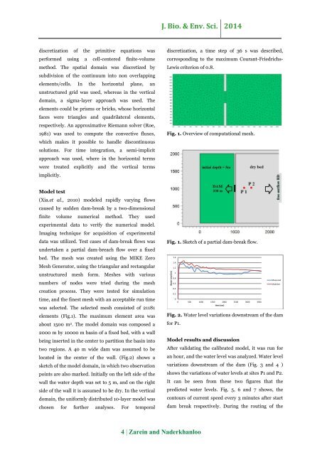
Fig. 1. Overview of computational mesh.
Model test
(Xia.et al., 2010) modeled rapidly varying flows
caused by sudden dam-break by a two-dimensional
finite volume numerical method. They used
experimental data to verify the numerical model.
Imaging technique for acquisition of experimental
data was utilized. Test cases of dam-break flows was
undertaken a partial dam-breach flow over a fixed
bed. The mesh was created using the MIKE Zero
Mesh Generator, using the triangular and rectangular
unstructured mesh form. Meshes with various
numbers of nodes were tried during the mesh
creation process. They were tested for simulation
time, and the finest mesh with an acceptable run time
was selected. The selected mesh consisted of 21181
elements (Fig.1). The maximum element area was
about 1500 m 2 . The model domain was composed a
2000 m by 10000 m basin of a fixed bed, with a wall
being inserted in the center to partition the basin into
two regions. A 40 m wide dam was assumed to be
located in the center of the wall. (Fig.2) shows a
sketch of the model domain, in which two observation
points are also marked. Initially on the left side of the
wall the water depth was set to 5 m, and on the right
side of the wall it is assumed to be dry. In the vertical
domain, the uniformly distributed 10-layer model was
chosen for further analyses. For temporal
Fig. 1. Sketch of a partial dam-break flow.
1.6
1.4
1.2
1
0.8
Measured
0.6
Modeled
0.4
0.2
0
0 500 1000 1500 2000 2500 3000 3500
time (sec)
Fig. 2. Water level variations downstream of the dam
for P1.
Model results and discussion
After validating the calibrated model, it was run for
an hour, and the water level was analyzed. Water level
variations downstream of the dam (Fig. 3 and 4 )
shows the variations of water levels at sites P1 and P2.
It can be seen from these two figures that the
predicted water levels. Fig. 5, 6 and 7 shows, the
contours of current speed every 3 minutes after start
dam break respectively. During the routing of the
4 | Zarein and Naderkhanloo