Chapter 11--Rosgen Geomorphic Channel Design

United States 

Department of 

Agriculture 

Natural 

Resources 

Conservation 

Service 

Part 654 Stream Restoration Design 

National Engineering Handbook 

Chapter 11 Rosgen Geomorphic 

Channel Design

Chapter 11 

Advisory Note 

Rosgen Geomorphic Channel Design 

Issued August 2007 

(210–VI–NEH, August 2007) 

Part 654 


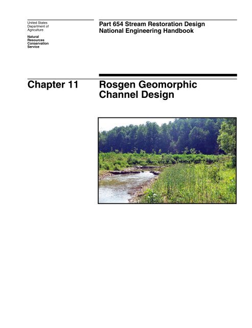
Cover photo: Stream restoration project, South Fork of the Mitchell River, 

NC, three months after project completion. The Rosgen 

natural stream design process uses a detailed 40-step 

approach. 

Techniques and approaches contained in this handbook are not all-inclusive, nor universally applicable. Designing 

stream restorations requires appropriate training and experience, especially to identify conditions where various 

approaches, tools, and techniques are most applicable, as well as their limitations for design. Note also that product 

names are included only to show type and availability and do not constitute endorsement for their specific use. 

The U.S. Department of Agriculture (USDA) prohibits discrimination in all its programs and activities on the basis 

of race, color, national origin, age, disability, and where applicable, sex, marital status, familial status, parental 

status, religion, sexual orientation, genetic information, political beliefs, reprisal, or because all or a part of an 

individual’s income is derived from any public assistance program. (Not all prohibited bases apply to all programs.) 

Persons with disabilities who require alternative means for communication of program information (Braille, large 

print, audiotape, etc.) should contact USDA’s TARGET Center at (202) 720–2600 (voice and TDD). To file a complaint 

of discrimination, write to USDA, Director, Office of Civil Rights, 1400 Independence Avenue, SW., Washington, 

DC 20250–9410, or call (800) 795–3272 (voice) or (202) 720–6382 (TDD). USDA is an equal opportunity provider 

and employer.

Chapter 11 Rosgen Geomorphic Channel Design 

Contents 

654.1100 Purpose 11–1 

654.1101 Introduction 11–1 

654.1102 Restoration phases 11–4 

(a) Phase I—Restoration objectives ...................................................................11–4 

(b) Phase II—Developing local and regional relations in geomorphic ..........11–4 

characterization, hydrology, and hydraulics 

(c) Phase III—Watershed and river assessment .............................................11–12 

(d) Phase IV—Passive recommendations for restoration .............................11–26 

(e) Phase V—The stream restoration and natural channel design using ....11–26 

the Rosgen geomorphic channel design methodology 

(f) Phase VI—Selection and design of stabilization and enhancement .......11–58 

structures/methodologies 

(g) Phase VII—Design implementation ............................................................11–70 

(h) Phase VIII—Monitoring and maintenance ................................................11–71 

654.1103 Conclusion 11–75 

Mathematical Definitions 11–76 

Tables Table 11–1 Valley types used in geomorphic characterization 11–5 

Table 11–2 General stream type descriptions and delineative criteria 11–8 

for broad-level classification (level 1) 

Table 11–3 Reference reach summary data form 11–9 

Table 11–4 Stream channel stability assessment summary form 11–25 

Table 11–5 Field procedure for bar samples 11–32 

Table 11–6 Field procedure for pavement/sub-pavement samples 11–33 

Table 11–7 Bar sample data collection and sieve analysis form 11–34 

Table 11–8 Sediment competence calculation form to assess bed 11–35 

stability (steps 23–26) 

Table 11–9 Data required to run the FLOWSED and POWERSED 11–37 

sediment transport models 

Table 11–10 FLOWSED model procedure to calculate annual bed- 11–43 

load and suspended sediment yield 


11–i



11–ii (210–VI–NEH, August 2007) 

Part 654 


Table 11–11 FLOWSED calculation of total annual sediment yield 11–44 

Table 11–12 POWERSED procedural steps of predicted bed-load and 11–50 

suspended sand-bed material transport changes due to 

alterations of channel dimension or slope (same stream 

with different bankfull discharges) 

Table 11–13 POWERSED model to predict bed-load and suspended 11–52 

sand-bed material load transport 

Table 11–14 Morphological characteristics of the existing and pro- 11–54 

posed channel with gage station and reference reach data 

Table 11–15 Equations for predicting ratio of vane length/bankfull 11–69 

width (VL) as a function of ratio of radius of curvature/ 

width and departure angle, where W = bankfull width 

(SI units) 

Table 11–16 Equations for predicting ratio of vane spacing/width 11–69 

(Vs) as a function of ratio of radius of curvature/width 

and departure angle, where W = bankfull width (SI units) 

Figures Figure 11–1 River restoration using Rosgen geomorphic channel 11–3 

design approach 

Figure 11–2 Broad-level stream classification delineation showing 11–6 

longitudinal, cross-sectional, and plan views of major 

stream types 

Figure 11–3 Classification key for natural rivers 11–7 

Figure 11–4 Regional curves from stream gaging stations showing 11–10 

bankfull discharge (ft 3 /s) vs. drainage area (mi 2 ) 

Figure 11–5 Regional curves from stream gage stations showing 11–11 

bankfull dimensions (width, depth, and cross-sectional area) 

vs. drainage area (mi 2 ) 

Figure 11–6 Relation of channel bed particle size to hydraulic 11–13 

resistance with river data from a variety of eastern and 

western streams 

Figure 11–7 Prediction of Manning’s n roughness coefficient 11–14 

Figure 11–8 Bankfull stage roughness coefficients (n values) by 11–15 

stream type for 140 streams in the United States and 

New Zealand




Part 654 


Figure 11–9 Dimensionless flow-duration curve for streamflow in 11–16 

the upper Salmon River area 

Figure 11–10 Generalized flowchart of application of various 11–17 

assessment levels of channel morphology, stability 

ratings, and sediment supply 

Figure 11–11 Relation between grain diameter for entrainment and 11–19 

shear stress using Shields relations 

Figure 11–12 Comparison of predicted sediment rating curve to observed 11–20 

values from the Tanana River, AK, using the Pagosa Springs 

dimensionless ratio relation 

Figure 11–13 Predicted vs. measured sediment data using reference 11–21 

dimensionless rating curve 

Figure 11–14 Predicted vs. measured suspended sediment data using 11–22 

dimensionless reference curve 

Figure 11–15 Various stream type succession scenarios 11–24 

Figure 11–16 Generalized flowchart representing Rosgen geomor- 11–27 

phic channel design utilizing analog, analytical, and 

empirical methodologies 

Figure 11–17 Flowchart for determining sediment supply and stabil- 11–28 

ity consequences for river assessment 

Figure 11–18 Generalized flowchart depicting procedural steps for 11–31 

sediment competence calculations 

Figure 11–19 General overview of the FLOWSED model 11–41 

Figure 11–20 Graphical depiction of the FLOWSED model 11–42 

Figure 11–21 Dimensionless flow-duration curve for Weminuche 11–45 

Creek, CO 

Figure 11–22 Bed-load sediment rating curve for Weminuche Creek, 11–45 

CO 

Figure 11–23 Suspended sediment rating curve for Weminuche Creek, 11–45 

CO 

Figure 11–24 Dimensioned flow-duration curve for Weminuche Creek, 11–45 

CO 

Figure 11–25 POWERSED prediction of bed-load and suspended sand- 11–48 

bed material load transport change due to alteration of 

channel dimension, pattern, or shape 

Figure 11–26 Graphical depiction of POWERSED model 11–49 

11–iii



11–iv (210–VI–NEH, August 2007) 

Part 654 


Figure 11–27 Cross section, profile, and plan view of a cross vane 11–59 

Figure 11–28 Cross vane installed on the lower Blanco River, CO 11–60 

Figure 11–29 Cross vane structure with step on the East Fork Piedra 11–60 

River, CO 

Figure 11–30 Cross vane/step-pool on the East Fork Piedra River, CO 11–60 

Figure 11–31 Cross vane/rootwad/log vane step-pool, converting a 11–60 

braided D4→C4 stream type on the East Fork Piedra 

River, CO 

Figure 11–32 Plan, cross section, and profile views of a W-weir 11–61 

structure 

Figure 11–33 W-weir installed on the Uncompahgre River, CO 11–61 

Figure 11–34 Plan, profile, and section views of the J-hook vane 11–62 

structure 

Figure 11–35 Log vane/J-hook combo with rootwad structure 11–63 

Figure 11–36 Rock vane/J-hook combo with rootwad and log vane 11–64 

footer 

Figure 11–37 Native boulder J-hook with cut-off sill, East Fork 11–65 

Piedra River, CO 

Figure 11–38 Rootwad/log vane/J-hook structure, East Fork Piedra 11–65 

River, CO 

Figure 11–39 J-hook/log vane/log step with cut-off sill, East Fork 11–65 


Figure 11–40 Longitudinal profile of proposed C4 stream type show- 11–66 

ing bed features in relation to structure location 

Figure 11–41 Boulder cross vane and constructed bankfull bench 11–67 

Figure 11–42 Locations/positions of rocks and footers in relation to 11–68 

channel shape and depths 

Figure 11–43 Rock size 11–69

Chapter 11 Rosgen Geomorphic Channel Design 

654.1100 Purpose 

This chapter outlines a channel design technique 

based on the morphological and morphometric qualities 

of the Rosgen classification system. While this 

approach is written in a series of steps, it is not a 

cookbook. This approach is often referred to as the 

Rosgen design approach. The essence for this design 

approach is based on measured morphological relations 

associated with bankfull flow, geomorphic valley 

type, and geomorphic stream type. This channel 

design technique involves a combination of hydraulic 

geometry, analytical calculation, regionalized validated 

relationships, and analogy in a precise series of steps. 

While this technique may appear to be straightforward 

in its application, it actually requires a series of precise 

measurements and assessments. It is important for the 

reader to recognize that the successful application of 

this design approach requires extensive training and 

experience. 

The contents of this chapter were submitted to the 

technical editors of this handbook as a manuscript 

titled Natural Channel Design Using a Geomorphic 

Approach, by Dave Rosgen, Wildland Hydrology, Fort 

Collins, Colorado. This material was edited to fit the 

style and format of this handbook. The approaches 

and techniques presented herein are not universally 

applicable, just as other approaches and techniques 

presented in this handbook are not necessarily appropriate 

in all circumstances. However, the Rosgen 

Geomorphic Approach for Natural Channel Design has 

been implemented in many locations and is cited as 

the methodology of choice for stream restoration by 

several state and local governments. 

654.1101 Introduction 

River restoration based on the principles of the Rosgen 

geomorphic channel design approach is most 

commonly accomplished by restoring the dimension, 

pattern, and profile of a disturbed river system by 

emulating the natural, stable river. Restoring rivers 

involves securing their physical stability and biological 

function, rather than the unlikely ability to return 

the river to a pristine state. Restoration, as used in 

this chapter, will be used synonymously with the term 

rehabilitation. Any river restoration design must first 

identify the multiple specific objectives, desires, and 

benefits of the proposed restoration. The causes and 

consequences of stream channel problems must then 

be assessed. 

Natural channel design using the Rosgen geomorphic 

channel design approach incorporates a combination 

of analog, empirical, and analytical methods for 

assessment and design. Because all rivers within a 

wide range of valley types do not exhibit similar morphological, 

sedimentological, hydraulic, or biological 

characteristics, it is necessary to group rivers of similar 

characteristics into discreet stream types. Such 

characteristics are obtained from stable reference 

reach locations by discreet valley types, and then are 

converted to dimensionless ratios for extrapolation to 

disturbed stream reaches of various sizes. 

The proper utilization of this approach requires fundamental 

training and experience using this geomorphic 

method. Not only is a strong background in geomorphology, 

hydrology, and engineering required, but the 

restoration specialist also must have the ability to 

implement the design in the field. The methodology is 

divided into eight major sequential phases: 

I Define specific restoration objectives associated 

with physical, biological, and/or chemical 

process. 

II Develop regional and localized specific information 

on geomorphologic characterization, 

hydrology, and hydraulics. 

III Conduct a watershed/river assessment to 

determine river potential; current state; and 

the nature, magnitude, direction, duration, 

and consequences of change. Review land 

(210–VI–NEH, August 2007) 11–1


use history and time trends of river change. 

Isolate the primary causes of instability 

and/or loss of physical and biological function. 

Collect and analyze field data including 

reference reach data to define sedimentological, 

hydraulic, and morphological parameters. 

Obtain concurrent biological data 

(limiting factor analysis) on a parallel track 

with the physical data. 

IV Initially consider passive restoration recommendations 

based on land use change in lieu 

of mechanical restoration. If passive methods 

are reasonable to meet objectives, skip 

to the monitoring phase (VIII). If passive efforts 

and/or recovery potential do not meet 

stated multiple objectives, proceed with the 

following phases. 

V Initiate natural channel design with subsequent 

analytical testing of hydraulic and 

sediment transport relations (competence 

and capacity). 

VI Select and design stabilization/enhancement/vegetative 

establishment measures and 

materials to maintain dimension, pattern, 

and profile to meet stated objectives. 

VII Implement the proposed design and stabilization 

measures involving layout, water 

quality control, and construction staging. 

VIII Design a plan for effectiveness, validation, 

and implementation monitoring to ensure 

stated objectives are met, prediction methods 

are appropriate, and the construction is 

implemented as designed. Design and implement 

a maintenance plan. 

The conceptual layout for the phases of the Rosgen 

geomorphic channel design approach is shown in 

figure 11–1. The various phases listed above are indicated 

on this generalized layout. The flowchart is 

indicative of the full extent and complexity associated 

with this method. 

Because of the complexity and uncertainty of natural 

systems, it becomes imperative to monitor each restoration 

project. The following are three objectives of 

such monitoring: 

• Ensure correct implementation of the design 

variables and construction details. 


11–2 (210–VI–NEH, August 2007) 

Part 654 


• Validate the analog, empirical, and analytical 

methods used for the assessment and design. 

• Determine effectiveness of the restoration 

methods to the stated physical and biological 

restoration objectives.


11–3 

Figure 11–1 River restoration using Rosgen geomorphic channel design approach 

Base 

level 

change 

Geomorphic characterization 

Valley type 

Cause of instability (land use/disturbance) 

Direct 

disturbance 

Riparian 

vegetation 

Recovery potential by 

mitigation/vegetation 

management change 

Visual/aesthetics, variation in 

type and materials used for 

stabilization/enhancement 

Riparian vegetation 

recommendations 

• Bioengineering 

• Transplants 

• Management 

Sediment 

competence/ 

capacity 

Stream type 

Streamflow 

change 

Potential stable stream 

type for valley type 

Change overall management (no direct or active 

construction-passive restoration) (Phase IV) 

Hydraulic relations 

(resistance, shear 

stress, stream power) 

Restoration goal/objectives (Phase I) 

Regional and local relations (Phase II) 

Streambank 

erosion 

prediction 

Stability examination 

nature of instability 

Successional 

scenarios/ 

stage of adjustment/ 

existing state 

Mitigation and/or 

restoration 

alternatives 

Mechanical or direct change 

in dimension, pattern, profile 

and/or materials 

Stream restoration/natural channel design (Phase V) 

Sediment 

competence 

calculation 

Sediment 

capacity 

calculation 

Hydrology: Regional curves bankfull calibration 

USGS gage data, hydraulic relations 

Watershed/river Assessment 

(Phase III) 

Reference reach by stream 

type/valley type. Mean values 

and natural variability of channel 

• Dimension, pattern profile 

• Dimensionless ratios 

Convert dimensionless ratios to 

actual values for design unique 

to a given stream type, flow, 

and material 

Design stabilization and fishery enhancement 

structures (to maintain stability, improve habitat, 

and extend period for riparian vegetation 

establishment) (Phase VI) 

Biological 

assessments 

Limiting factor 

analysis 

Recommendations 

for channel 

features, habitat 

requirements, and 

habitat diversity 

Final design Implementation (Phase VII) Monitoring and maintenance (Phase VIII) 



Part 654 

National Engineering Handbook


654.1102 Restoration phases 

(a) Phase I—Restoration objectives 

It is very important to obtain clear and concise statements 

of restoration objectives to appropriately design 

the solution(s). The potential of a certain stream to 

meet specific objectives must be assessed early on 

in the planning phases so that the initial restoration 

direction is appropriate. The common objectives are: 

• flood level reduction 

• streambank stability 

• reduce sediment supply, land loss, and attached 

nutrients 

• improve visual values 

• improve fish habitat and biological diversity 

• create a natural stable river 

• withstand floods 

• be self-maintaining 

• be cost-effective 

• improve water quality 

• improve wetlands 

It is essential to fully describe and understand the 

restoration objectives. The importance of formulating 

clear, achievable, and measurable objectives is 

described in detail in NEH654.02. Often the objectives 

can be competing or be in conflict with one another. 

Conflict resolution must be initiated and can often be 

offset by varying the design and/or the nature of stabilization 

methods or materials planned. 

The assessment required must also reflect the restoration 

objectives to ensure various related processes are 

thoroughly evaluated. For example, if improved fishery 

abundance, size, and species are desired, a limiting 

factor analysis of habitat and fish populations must be 

linked with the morphological and sedimentological 

characteristics. 



Part 654 


(b) Phase II—Developing local and 

regional relations in geomorphic 

characterization, hydrology, and 

hydraulics 

Geomorphic characterization 

The relations mapped at this phase are the geomorphic 

characterization and description levels for stream 

classification (Rosgen 1994, 1996). Valley types (table 

11–1) are mapped prior to stream classification to 

ensure reference reach data are appropriately applied 

for the respective valley types being studied. 

Morphological relations associated with stream types 

are presented in figures 11–2 (Rosgen 1994) and 

11–3 (Rosgen 1996) and summarized in table 11–2. In 

natural channel design using the Rosgen geomorphic 

channel design approach, it is often advantageous to 

have an undisturbed and/or stable river reach immediately 

upstream of the restoration reach. Reference 

reach data are obtained and converted to dimensionless 

ratio relations to extrapolate channel dimension, 

pattern, profile, and channel material data to rivers 

and valleys of the same type, but of different size. If an 

undisturbed/stable river reach is not upstream of the 

restoration reach, extrapolation of morphological and 

dimensionless ratio relations by valley and stream type 

is required for both assessment and design. 

An example of the form used to organize reference 

reach data, including dimensionless ratios for a given 

stream type, is presented in table 11–3. Specific design 

variables use reference reach data for extrapolation 

purposes, assuming the same valley and stream type 

as represented. These relations are only representative 

of a similar stable stream type within a valley type of 

the disturbed stream. 

Hydrology 

The hydrology of the basin is often determined from 

regional curves constructed from long-term stream 

gage records. Relationships of flow-duration curves 

and flood-frequency data are used for computations in 

both the assessment and design phases. Stream Hydrology 

is also addressed in NEH654.05. Relations are 

converted to dimensionless formats using bankfull discharge 

as the normalization parameter. Bankfull discharge 

and dimensions associated with stream gages 

are plotted as a function of drainage area for extrapolation 

to ungaged sites in similar hydro-physiographic 

provinces. A key requirement in the development of



Table 11–1 Valley types used in geomorphic characterization 

Valley types Summary description of valley types 

I Steep, confined, V-notched canyons, rejuvenated side slopes 

II Moderately steep, gentle-sloping side slopes often in colluvial valleys 

III Alluvial fans and debris cones 

IV Gentle gradient canyons, gorges, and confined alluvial and bedrock-controlled valleys 

V Moderately steep, U-shaped glacial-trough valleys 

VI Moderately steep, fault, joint, or bedrock (structural) controlled valleys 

VII Steep, fluvial dissected, high-drainage density alluvial slopes 

VIII 

Wide, gentle valley slope with well-developed flood plain adjacent to river and/or glacial 

terraces 


Part 654 


IX Broad, moderate to gentle slopes, associated with glacial outwash and/or eolian sand dunes 

X 

XI Deltas 

Very broad and gentle valley slope, associated with glacio- and nonglacio-lacustrine 

deposits 

11–5


Figure 11–2 Broad-level stream classification delineation showing longitudinal, cross-sectional, and plan views of major stream types 



Part 654 




Figure 11–3 Classification key for natural rivers 



Part 654 





Part 654 


Table 11–2 General stream type descriptions and delineative criteria for broad-level classification (level 1) 

Stream 

type 

General 

description 

Aa+ Very steep, deeply entrenched, 

debris transport, torrent streams 

A Steep, entrenched, cascading, 

step-pool streams. High energy/ 

debris transport associated with 

depositional soils. Very stable if 

bedrock or boulder-dominated 

channel 

B Moderately entrenched, moderate 

gradient, riffle dominated channel 

with infrequently spaced pools. 

Very stable plan and profile. 

Stable banks 

C Low gradient, meandering, 

point bar, riffle/pool, alluvial 

channels with broad, well-defined 

flood plains 

D Braided channel with longitudinal 

and transverse bars. 

Very wide channel with 

eroding banks 

DA Anastomizing (multiple channels) 

narrow and deep with extensive, 

well-vegetated flood plains and 

associated wetlands. Very gentle 

relief with highly variable sinuosities 

and width-to-depth ratios. Very stable 

streambanks 

E Low gradient, meandering riffle/pool 

stream with low width-to-depth ratio 

and little deposition. Very efficient 

and stable. High meander width ratio 

F Entrenched meandering riffle/pool 

channel on low gradients with 

high width-to-depth ratio 

G Entrenched gully step-pool and 

low width-to-depth ratio on moderate 

gradients 

Entrenchment 

ratio 

W/d 

ratio Sinuosity Slope 

Landform/ 

soils/features 

2.2 >12 >1.2 40 n/a 2.2 Highly 

variable 

Highly 

variable 

2.2 1.5 1.2


Table 11–3 Reference reach summary data form 

Channel dimension 

Channel pattern 

Channel profile 

Channel materials 


River Reach Summary Data 

Mean riffle depth (dbkf) ft Riffle width (Wbkf) ft 

Riffle area (A bkf) 

Mean pool depth (dbkfp) ft Pool width (Wbkfp) ft Pool area (Abkfp) Mean pool depth/mean d / bkfp Wbkfp Pool area/riffle 

Pool width/riffle width 

riffle depth (dbkf) /Wbkf area 

Max riffle depth (dmbkf) ft Max pool depth (d ) mbkfp ft Max riffle depth/mean riffle depth 

Max pool depth/mean riffle depth Point bar slope 

Streamflow: estimated mean velocity at bankfull stage (u bkf) ft/s Estimation method 

Streamflow: estimated discharge at bankfull stage (Qbkf) ft3 /s mi2 Drainage area 

Geometry Mean Min. Max. Dimensionless geometry ratios Mean Min. Max. 

Meander length (Lm) 

ft 

Meander length ratio (Lm/W bkf) 

Radius of curvature (Rc) ft Radius of curvature/riffle width (Rc/W bkf) 

Belt width (W blt) ft Meander width ratio (W blt/W bkf) 

Individual pool length ft Pool length/riffle width 

Pool to pool spacing ft Pool to pool spacing/riffle width 

Valley slope (VS) ft/ft 

Facet slopes Mean Min. Max. Dimensionless geometry ratios Mean Min. Max. 

% Silt/clay 

Geometry Reach b/ Riffle c/ Bar Reach b/ Riffle c/ Bar 

% Sand D 35 

% Gravel D 50 

% Cobble D 84 

% Bedrock 

Average water surface slope (S) ft/ft 

Stream length (SL) ft Valley length (VL) 

ft 

Low bank height start 

(LBH) end 

ft 

ft 

% Boulder D 95 

a/ Minimum, maximum, mean depths are the average midpoint values except pools which are taken at deepest part of pool 

b/ Composite sample of riffles and pools within the designated reach 

c/ Active bed of a riffle 

D 16 

D 100 


Sinuosity (VS/S) 

Sinuosity (SL/VL) 

Max riffle start ft Bank height ratio 

depth 

end ft (LBH/max riffle depth) 

Riffle slope (S rif) ft/ft Riffle slope/average water surface slope (S rif/S) 

Run slope (S run) ft/ft Run slope/average water surface slope (S run/S) 

Pool slope (S p) ft/ft Pool slope/average water surface slope (S p/S) 

Glide slope (S g) ft/ft Glide slope/average water surface slope (S g/S) 

Feature midpoint a/ Mean Min. Max. Dimensionless geometry ratios Mean Min. Max. 

Riffle depth (d rif) ft Riffle depth/mean riffle depth (d rif/d bkf) 

Run depth (d run) ft Run depth/mean riffle depth (d run/d bkf) 

Pool depth (d p) ft Pool depth/mean riffle depth (d p/d bkf) 

Glide depth (d g) ft Glide depth/mean riffle depth (d g/d bkf) 

Part 654 


start 

end 

ft 2 

ft 2 

A / bkfp 

Abkf mm 

mm 

mm 

mm 

mm 

mm 



such relations is the necessity to field-calibrate the 

bankfull stage at each gage within a hydro-physiographic 

province (a drainage basin similar in precipitation/runoff 

relations due to precipitation/elevation, 

lithology and land uses). 

Regional curves—The field-calibrated bankfull stage 

is used to obtain the return period associated with the 

bankfull discharge. Regional curves of bankfull discharge 

versus drainage area are developed (fig. 11–4) 

(adapted from Dunne and Leopold 1978)). To plot 

bankfull dimensions by drainage area, the U.S. Geological 

Survey (USGS) 9–207 data (summary of stream 



Part 654 


discharge measurements at the gage) are obtained to 

plot the at-a-station hydraulic geometry relations (fig. 

11–5 (adapted from Rosgen 1996; Rosgen and Silvey 

2005)). These data are then converted to dimensionless 

hydraulic geometry data by dividing each value 

by their respective bankfull value. These relations are 

used during assessment and design to indicate the 

shape of the various cross sections from low flow to 

high flow. In the development of the dimensionless 

hydraulic geometry data, current meter measurements 

must be stratified by stream type (Rosgen 1994, 1996) 

and for specific bed features such as riffles, glides, 

runs, or pools. 

Figure 11–4 Regional curves from stream gaging stations showing bankfull discharge (ft 3 /s) vs. drainage area (mi 2 ) 

Bankfull discharge (ft 3 /s) 

5,000 

4,000 

3,000 

2,000 

1,000 

500 

400 

300 

200 

100 

50 

40 

30 

20 

Bankfull discharge as a function 

of drainage area for several 

regions in the U.S. 

10 

.2 .3 .4 .5 1 2 3 4 5 10 

West Cascades and Puget Lowlands, WA 

San Francisco Bay region (areas of 30-in/yr precipitation) 

Southeast PA 

Upper Green River, WY 

Drainage area (mi 2 ) 

5,000 

4,000 

3,000 

2,000 

1,000 

500 

400 

300 

200 

100 

50 

40 

10 

20 30 40 50 100 200 300 400500 1,000 

30 

20




Part 654 


Figure 11–5 Regional curves from stream gage stations showing bankfull dimensions (width, depth, and cross-sectional 

area) vs. drainage area (mi 2 ) 

Mean depth (ft) Width (ft) 

Cross-sectional area (ft2 ) 

100 

.1 

3,000 

2,000 

.2 .3 .4 .5 1 2 3 4 5 10 20 30 40 50 

1,000 

500 

400 

300 

200 

100 

50 

40 

30 

20 

10 

5 

4 

3 

2 

1 

50 

40 

30 

20 

10 

5 

4 

3 

2 

1 

Bankfull channel dimensions 

.5 

.1 .2 .3 .4 .5 1 2 3 4 5 10 

Drainage area (mi 2 ) 

20 30 40 50 

100 

San Francisco Bay region (@ 30-in annual precipation) 

Eastern United States 

Upper Green River, WY (Dunne and Leopold 1978) 

Upper Salmon River, ID (Emmett 1975) 

200 

300 

400 

500 

200 

300 

400 

500 

1,000 

1,000 

3,000 

2,000 

1,000 

500 

400 

300 

200 

100 

50 

40 

30 

20 

500 

400 

300 

200 

100 

50 

40 

30 

10 

5 

4 

3 

2 

1 

.5 

Cross-sectional area (ft 2 ) 

Width (ft) 

Mean depth (ft) 

11–11


Hydraulic relations 

Hydraulic relations are validated using resistance 

equations for velocity prediction at ungaged sites. 

(Stream Hydraulics is addressed in more detail in 

NEH654.06) Validation is accomplished by back calculating 

relative roughness (R/D 84 ) and a friction factor 

(u/u * ) from actual measured velocity for a range of 

streamflows including bankfull: 

⎡ 

⎛ R ⎞ ⎤ 

u = ⎢2. 

83 + 5. 66 log u 

⎝ 

⎜ D ⎠ 

⎟ ⎥ * 

⎣⎢ 

84 ⎦⎥ 

where: 

(eq. 11–1) 

u = mean velocity (ft/s) 

R = hydraulic radius 

D = diameter of bed material of the 84th percentile 

84 

of riffles 

u * = shear velocity (gRS)½ 

g = gravitational acceleration 

S = slope 

Measured velocity, slope, channel material, and hydraulic 

radius data from various Colorado rivers using 

this friction factor (u/u * ) and relative roughness 

(R/D 84 ) relation are shown in figure 11–6 (Rosgen, Leopold, 

and Silvey 1998; Rosgen and Silvey 2005). 

Manning’s n (roughness coefficient) can also be 

back-calculated from measured velocity, slope, and 

hydraulic radius. Another approach to predict velocity 

at ungaged sites is to predict Manning’s n from a 

friction factor back-calculated from relative roughness 

shown in figure 11–7 (Rosgen, Leopold, and Silvey 

1998; Rosgen and Silvey 2005). Manning’s n can also 

be estimated at the bankfull stage by stream type as 

shown in the relationship from gaged, large streams 

in figure 11–8. Vegetative influence is also depicted in 

these data (Rosgen 1994). 

Dimensionless flow-duration curves—Flow-duration 

curves (based on mean daily discharge) are also 

obtained from gage stations then converted to dimensionless 

form using bankfull discharge as the normalization 

parameter (fig. 11–9 (Emmett 1975)). The 

purpose of this form is to allow the user to extrapolate 

flow-duration curves to ungaged basins. This relationship 

is needed for the annual suspended and bed-load 

sediment yield calculation along with channel hydraulic 

variables. 



Part 654 


(c) Phase III—Watershed and river 

assessment 

Land use history is a critical part of watershed assessment 

to understand the nature and extent of potential 

impacts to the water resources. Past erosional/depositional 

processes related to changes in vegetative cover, 

direct disturbance, and flow and sediment regime 

changes provide insight into the direction and detail 

for assessment procedures required for restoration. 

Time series of aerial photos are of particular value to 

understand the nature, direction, magnitude, and rate 

of change. This is very helpful, as it assists in assessing 

both short-term, as well as long-term river problems. 

Assessment of river stability and sediment 

supply 

River stability (equilibrium or quasi-equilibrium) is defined 

as the ability of a river, over time, in the present 

climate to transport the flows and sediment produced 

by its watershed in such a manner that the stream 

maintains its dimension, pattern, and profile without 

either aggrading or degrading (Rosgen 1994, 1996, 

2001d). A stream channel stability analysis is conducted 

along with riparian vegetation inventory, flow 

and sediment regime changes, limiting factor analysis 

compared to biological potential, sources/causes of 

instability, and adverse consequences to physical and 

biological function. Procedures for this assessment are 

described in detail by Rosgen (1996, 2001d) and in Watershed 

Assessment and River Stability for Sediment 

Supply (WARSSS) (Rosgen 1999, 2005). 

It is important to realize the difference between the 

dynamic nature of streams and natural adjustment 

processes compared to an acceleration of such adjustments. 

For example, bank erosion is a natural 

channel process; however, accelerated streambank 

erosion must be understood when the rate increases 

and creates a disequilibrium condition. Many stable 

rivers naturally adjust laterally, such as the “wandering” 

river. While it may meet certain local objectives to 

stabilize high risk banks, it would be inadvisable to try 

to “control” or “fix in place” such a river. 

In many instances, a braided river and/or anastomizing 

river type is the stable form. Designing all stream 

systems to be a single-thread meandering stream may 

not properly represent the natural stable form. Valley 

types are a key part of river assessment to understand




Part 654 


Figure 11–6 Relation of channel bed particle size to hydraulic resistance with river data from a variety of eastern and western 

streams 

Resistance (friction) factor, u/u * 

16 

15 

14 

13 

12 

11 

10 

9 

8 

7 

6 

5 

4 

3 

2 

1 

⎡ 

⎛ R ⎞ ⎤ 

u = ⎢2. 

83 + 5. 66 log u 

⎝ 

⎜ D ⎠ 

⎟ ⎥ 

⎣⎢ 

84 ⎦⎥ 

Limerinos 1970 

Leopold, Wolman, and Miller 1964 

0 

0 

.5 1 2 3 4 5 10 20 30 40 50 100 

Relative roughness 

Ratio of hydraulic mean depth to channel bed material size, 

R/D 84 

* 

1 

6 

5 

4 

3 

f 

2 

1 



Figure 11–7 Prediction of Manning’s n roughness coefficient 

Manning’s roughness coefficient n 

1.00 

.90 

.80 

.70 

.60 

.50 

.40 

.30 

.20 

.10 

.09 

.08 

.07 

.06 

.050 

.045 

.040 

.035 

.030 

.025 

= ( ) 

τ 

* 

u shear velocity= γRs 

0 

= shear stress= γ Rs 

= 

f 

⎛ ⎞ 

⎝ 

⎜ 

⎠ 

⎟ = 

u 

u * 

8 

γR s 

f = 

u 

8 

2 

u 

τ 

ρ 

0 

Reference notes 

n = Manning’s roughness coefficient 

A = cross-sectional area 

g = gravitational acceleration 

R = hydraulic radius (area/wet. perim.) 

(ft), (aka. hydraulic mean depth) 

D84 = grain diameter or particle size at 

the 84th percentile index 

γ = specific weight of water (62.4 lb/ft3 ) 

/g = slug = 1.94/ft3 water (1 slug = 32.174 lb mass) 

ρ = mass density of fluid (lb mass/ft3 ) 

mass density of water = 1.94 slugs/ft3 γ 

.020 

0 2 4 6 8 10 12 14 16 18 20 22 24 

Friction factor, u/u * 

u = mean velocity 

s = slope (ft/ft) 

Q = discharge (ft 3 /s) 

n = 0.39(s) .38 (R) -.16 

Q = 3.81(A × R) .83 s .12 

u = 3.81(R) .83 (s) .12 

Data Point Stream type 

C4 

B3 

A3, A2 

C5 

Rosgen (Western U.S.) 



Part 654 




Figure 11–8 Bankfull stage roughness coefficients (n values) by stream type for 140 streams in the United States and New Zealand 

Manning’s roughness coefficient n 

.20 

.10 

.09 

.08 

.07 

.06 

.05 

.04 

.03 

.02 

A3 A2 F2 G6 B2 B3 B5 

B6 

Roughness n = 

Velocity u = 

1,486 

Q (A)(R2/3 )(S 1/2 ) 

1,486 (R 2/3 )(S 1/2 ) 

n 

Reference notes 

n = 0.39(s) .38 (R) -.16 

u = 3.81(R) .83 (s) .12 

Average bankfull value for rivers of medium to large size 

B3c G5 F5 F6 G4 B4 F3 C5 E5 

E6 

Rosgen stream types 

B1 F4 E3 

E4 

Q = 3.81(A*R) .83 S .12 

Average bankfull value for smaller rivers with controlling vegetative influence 

G3 C1 C3 

C4 



Part 654 



which stream types are stable within a variety of valley 

types in their geomorphic settings. Reference reaches 

that represent the stable form have to be measured 

and characterized only for use in similar valley types. 

This prevents applying good data to the wrong stream 

type. 

Time-trend data using aerial photography is very valuable 

at documenting channel change. Field evidence 

using dendrochronology, stratigraphy, carbon dating, 

paleochannels, or evidence of avulsion and avulsion 

dates can help the field observer to understand rate, 

direction, and consequence of channel change. 

The field inventory and the number of variables required 

to conduct a watershed and river stability assessment 

is substantial. The flowchart in figure 11–10 

represents a general summary of the various elements 

used for assessing channel stability as used in this 

methodology. The assessment effort is one of the key 

procedural steps in a sound restoration plan, as it 

Figure 11–9 Dimensionless flow-duration curve for 

streamflow in the upper Salmon River area 

Ratio of discharge to bankfull discharge 

5 

2 

1 

0.5 

0.2 

0.1 

0.05 

0.02 

0.01 

.1 1 10 

20 40 60 80 90 99 99.9 

Duration in percentage of time 



Part 654 


identifies the causes and consequences of the problems 

leading to loss of physical and biological river 

function. Some of the major variables are described to 

provide a general overview. 

Streamflow change—Streamflow alteration (magnitude, 

duration, and timing) due to land use changes, 

such as percent impervious cover, must be determined 

at this phase. Streamflow models, such as the unit 

hydrograph approach, must be calibrated by back-calculating 

what precipitation probability generates bankfull 

discharge for various antecedent soil moisture and 

runoff curve numbers. It is critical to separate bankfull 

discharge from flood flows, as each flow category, including 

flood flow, has a separate dimension, pattern, 

and profile. This varies by stream type and the lateral 

and vertical constraints imposed within the valley (or 

urban “valley”). 

Flow-duration curves by similar hydro-physiographic 

provinces from gaged stations are converted to bankfull 

dimensionless flow duration for use in the annual 

sediment yield calculation. Snowmelt watershed flow 

prediction output (Troendle, Swanson, and Nankervis 

2005) is generally shown in flow-duration changes, 

rather than an annual hydrograph. Similar model 

outputs using flow-duration changes are shown in 

Water Resources Evaluation of Nonpoint Silvicultural 

Sources (U.S. Environmental Protection Agency (EPA) 

1980). 

Sediment competence—Sedimentological data are 

obtained by a field measurement of the size of bar and 

bed material, bed-load sediment transport, suspended 

sediment transport, and bankfull discharge measurements 

at the bankfull stage. Sediment relations are established 

by collecting energy slope, hydraulic radius, 

bed material, bar material, and the largest particle 

produced by the drainage immediately upstream of the 

assessment reach. Critical dimensionless shear stress 

is calculated from field data to determine sediment 

competence (ability to move the largest particle made 

available to the channel). Procedures for this field 

inventory are presented in Andrews (1984) and Rosgen 

(2001a, 2001d, 2005). Potential aggradation, degradation, 

and channel enlargement are predicted for the 

disturbed reach, comparing the required depth and 

slope necessary to transport the largest size sediment 

available. These calculations can be accomplished by 

hand, spreadsheet, or by commercially available computer 

programs.



Selection of representative 

reach for stability analysis 

Valley type (Level I) 

Field determined bankfull discharge/velocity estimation 

Stream type 

• W/d • Sinuosity (Level II) 

• Materials 

Dimensionless ratio relations of morphological variables 


Part 654 


Figure 11–10 Generalized flowchart of application of various assessment levels of channel morphology, stability ratings, and 

sediment supply 

Prediction of river stability and sediment supply based on condition categories, departure analysis, and sedimentological relations (Level III) 

Entrenchment 

Degree 

of 

incision 

Vertical stability (aggradation 

or degradation processes) 

Sediment 

capacity 

model 

Stream 

succession 

stage 

Channel 

enlargement 

• Entrenchment 

• Slope 

• W/d 

• Slope ratios 

Sediment 

competence 

W/d 

ratio 

state 

Sediment supply 

Depositional 

pattern 

Field validation procedure (Level IV) 

• Permanaent cross-sectional resurvey 

• Longitudinal profile survey 

• Channel materials resurvey 

*Optional: sediment measurements (largest size moved at bankfull, D i ) 

• Depth ratios 

• Lm/W 

Selection of representative reference 

reach for stability analysis 

• Rc/W 

• MWR (Level II) 

Meander 

pattern 

Lateral 

stability 

• Scour chain installation 

• Installation of bank pins/profile* 

• Time trend study (aerial photos) 

Confinement 

Gage station/ 

bankfullvalidation 

Regional curves 

Bank 

erosion 

prediction 

Pfankuch 

channel 

stability 



Changes in channel dimension, pattern, and profile 

are reflected in changes of velocity, depth, and slope. 

These changes in the hydraulic variables are reflected 

in values of shear stress. Shear stress is defined as: 

τ = γRS 


where: 

τ = bankfull shear stress (lb/ft 2 ) 

γ = specific weight of water = 62.4 lb/ft 3 

R = hydraulic radius of riffle cross section (ft) 

S = average water surface slope (ft/ft) 

Use the calculated value of τ (lb/ft 2 ) and the Shields 

diagram as revised with the Colorado data (fig. 11–11 

(Rosgen and Silvey 2005)) to predict the moveable 

particle size (mm) at bankfull shear stress. 

Another relationship used in assessment and in design 

is the use of dimensionless shear stress (τ * 

ci ) to determine 

particle entrainment. Dimensionless shear stress 

is defined as: 

τ * 

⎛ D 

= 0. 0834 ⎜ ^ 

⎝ D 

50 

50 

⎞ 

⎟ 

⎠ 

−0. 

872 



where: 

τ * = dimensionless shear stress 

D 50 = median diameter of the riffle bed (from 100 

count in the riffle or pavement sample) 

ˆD 50 = median diameter of the bar sample (or subpavement 

sample) 

If the ratio D50 

is between the values of 3.0 and 7.0, 

Dˆ 

50 

calculate the critical dimensionless shear stress using 

equation 11–3 (modifications adapted from Andrews 

1983, 1984; Andrews and Erman 1986). 

If the ratio D50 

is not between the values of 3.0 and 

Dˆ 

50 

7.0, calculate the ratio Dmax 

D50 

where: 

D = largest particle from the bar sample (or the 

max 

subpavement sample) 

D50 = median diameter of the riffle bed (from 100 

count in the riffle or the pavement sample) 

If the ratio Dmax 

is between the value of 1.3 and 3.0, 

D50 

calculate the critical dimensionless shear stress: 


τ 

Part 654 


⎛ D 

= 0. 0384 

⎝ 

⎜ D 

* max 

50 

⎞ 

⎠ 

⎟ 

−0. 

887 


Once the dimensionless shear stress is determined, 

the bankfull mean depth required for entrainment of 

the largest particle in the bar sample (or subpavement 

sample) is calculated using equation 11–5: 

d 

bkf 

D 

= 1 65 

S 

. 

* max 

τ (eq. 11–5) 

where: 

d = required bankfull mean depth (ft) 

bkf 

1.65 = submerged specific weight of sediment 

τ * 

= dimensionless shear stress 

D max = largest particle from bar sample (or subpavement 

sample) (ft) 

S = bankfull water surface slope (ft/ft) 

The bankfull water surface slope required for entrainment 

of the largest particle can be calculated using 

equation 11–6: 

* Dmax 

S = 1. 65τ 


d bkf 

Equations 11–5 and 11–6 are derived from the basic 

Shields relation. 

If the protrusion ratios are out of the usable range as 

stated, another option is to calculate sediment entrainment 

using dimensional bankfull shear stress (eq. 11–2 

and fig. 11–11). 

Sediment capacity—In addition to sediment competence, 

sediment capacity is important to predict 

river stability. Unit stream power is also utilized to 

determine the distribution of energy associated with 

changes in the dimension, pattern, profile, and materials 

of stream channels. Unit stream power is defined 

as shear stress times mean velocity: 

ω = τu 


where: 

ω = unit stream power (lb/ft/s) 

τ = shear stress (lb/ft 2 ) 

u = mean velocity (ft/s) 

Predicted sediment rating curves are converted to 

unit stream power for the same range of discharges by 

individual cells to demonstrate reduction or increase 

in coarse sediment transport.


1,000 

500 

400 

300 

200 

100 

50 

40 

30 

20 

10 

5 

4 

3 

2 

1 

.5 

.4 

.3 

.2 

.1 



Part 654 


Figure 11–11 Relation between grain diameter for entrainment and shear stress using Shields relations 

Grain diameter (mm) 

.001 

.002 

.003 

.004 

.005 

.01 

Colorado data: Power trendline 

.7355 

Dia. (mm) = 152.02 τc R2 = .838 

.01 

.1 1 

.02 .03.04 .1 .2 .3 .4 .5 1 2 3 4 5 10 

.05 

τ c = Critical shear stress (lb/ft 2 ) 

Laboratory and field data on critical shear stress required to initiate 

movement of grains (Leopold, Wolman, and Miller 1964). The solid line is the 

Shields curve of the threshold of motion; transposed from the θ versus R g 

form into the present form, in which critical shear is plotted as a function of 

grain diameter. 


Colorado data (Wildland Hydrology) 

Power trendline: 


1.042 

Dia. (mm) = 77.966τc R2 = .9336 

10 



The use of reference dimensionless sediment rating 

curves by stream type and stability rating, (Troendle et 

al. 2001), as well as hydrology and hydraulic data, are 

all needed for the stability and design phases. Additional 

information will be presented in the respective 

sequential, analytical steps of each phase of the procedure. 

Local suspended sediment and bed-load data can 

be converted to regional sediment curves by plotting 

bankfull and suspended sediment data by drainage 

area. Examples of suspended sediment data plotted by 

1.5-year recurrence interval discharge/drainage area 

for many regions of the United States as developed 

from USGS gage data by the U.S. Department of Agriculture 

(USDA), Agricultural Research Service (ARS) 

are presented in Simon, Dickerson, and Heins (2004). 

These relations can be used if a direct measurement 

of bankfull sediment cannot be obtained for subsequent 

analysis. Caution should be exercised in using 

an arbitrary bankfull value without field calibration of 

the bankfull discharge. The 1.5-year recurrence interval 

discharge is often greater than the actual bankfull 

value in wet climates and urban areas. 

The disadvantage of using various suspended and 

bed load equations for the Rosgen geomorphic channel 

design methodology is the difficulty of determining 

sediment supply for sediment rating curves. It is 

Suspended sediment conc (mg/L) 

5,000 

4,500 

4,000 

3,500 

3,000 

2,500 

2,000 

1,500 

1,000 

500 

Measured data 

Pagosa prediction 


0 

0 10,000 20,000 30,000 40,000 50,000 60,000 70,000 80,000 

Discharge (ft 3 /s) 


Part 654 


common in the use of these models to have predicted 

values of many orders of magnitude different than 

observed values. The use of developed dimensionless 

ratio sediment rating curves for both suspended (less 

wash load) and bed load by stream type and stability is 

the improvement of predicted versus observed values. 

Results of an independent test of predicted versus 

observed values for a variety of USGS gage sites 

are shown in figures 11–12, 11–13, and 11–14. These 

figures show that predicted sediment rating curves 

match observed values for a wide range of flows. The 

model for bed-load transport reflects sediment transport 

based on changes in the channel hydraulics from 

a reference condition. 

Validation of sediment competence or entrainment relations 

can also assist in the development and application 

of subsequent analysis. These data can be collected 

by installing scour chains and actual measurements 

of bed-load transport grain size for a given shear stress 

using Helley-Smith bed-load samplers. Plotting existing 

data collected by others in this manner can also 

help in developing a data base used in later analysis. 

The use of reference dimensionless ratio sediment 

rating curves (bed load and suspended less wash load) 

requires field measured bankfull sediment and dis- 

Figure 11–12 Comparison of predicted sediment rating curve to observed values from the Tanana River, AK, using the Pagosa 

Springs dimensionless ratio relation




Part 654 


Figure 11–13 Predicted vs. measured sediment data using reference dimensionless rating curve (data from Leopold and Emmett 

1997; Ryan and Emmett 2002) 

East Fork River near Big Sandy, WY (from Leopold and Emmett 1997) 

Unit bed-load transport (kg/m/s) 

Note: Fixed width at 

bedload cross 

section 

Little Granite Creek near Bondurant, WY (from Ryan and Emmett 2002) 

Bed-load transport (tons/d) 

0.25 

0.2 

0.15 

0.1 

0.05 

0 

0 10 20 30 

Discharge (m 3 /s) 

Measured data 


Reported curve 

Maggie Creek (F4)—NV 

Bed-load transport (tons/d) 

200 

150 

100 

50 

0 

140 

120 

100 

80 

60 

40 

20 

0 

0 100 200 300 


Measured data 


Power (measured) 

Measured data 



40 50 

400 500 

0 100 200 300 

Discharge (ft3 400 500 600 

/s) 

Suspended sediment (mg/L) 



0.25 

0.2 

0.15 

0.1 

0.05 

1,200 

1,000 

Measured data 



0 

0 5 10 15 20 30 

Discharge (m3 25 35 

/s) 

800 

600 

400 

200 

0 

6,000 

5,000 

4,000 

3,000 

2,000 

1,000 

0 

Measured data 


Reported curve 

0 100 200 300 


Measured data 



400 500 

0 100 200 300 

Discharge (ft3 400 500 600 700 

/s) 





Part 654 


Figure 11–14 Predicted vs. measured suspended sediment data using dimensionless reference curve (data from Emmett 

1975) 

Warm Springs Creek near Clayton, ID 13297000 Upper Salmon Watershed 13297250 


120 

100 

80 

60 

40 

20 

0 

Measured data 



0 100 200 300 


/s) 

Measured data 


Linear (measured) 

Upper Salmon Watershed 13297340 Upper Salmon Watershed 13297360 


Measured data 



Upper Salmon Watershed 13297380 Upper Salmon Watershed 13297425 


450 

400 

350 

300 

250 

200 

150 

100 

50 

0 

120 

100 

80 

60 

40 

20 

0 

0 100 200 300 


/s) 

Measured data 



0 2,000 4,000 

Discharge (ft3 /s) 

6,000 8,000 




2,500 

2,000 

1,500 

1,000 

500 

0 

0 20 40 60 80 120 

Discharge (ft3 100 

/s) 

700 

600 

500 

400 

300 

200 

100 

0 

400 

350 

300 

250 

200 

150 

100 

50 

0 

Measured data 



0 100 200 300 

Discharge (ft3 400 500 

600 

/s) 

Measured data 



0 500 1,000 

Discharge (ft3 1,500 2,000 2,500 

/s) 

3,000




Part 654 


Figure 11–14 Examples of predicted vs. measured suspended sediment data using dimensionless reference curve (data from 

Emmett 1975)—Continued 


Big Boulder Creek near Clayton, ID 13297500 East Fork Salmon River near Clayton, ID 13298000 

3,000 

2,500 

2,000 

1,500 

1,000 

500 

0 

0 50 100 150 


Measured data 



Measured data 



Little Boulder Creek near Clayton, ID 13297450 Salmon River near Challis, ID 13298500 


Measured data 



Salmon River below Yankee Fork 13296500 Yankee Fork Salmon River near Clayton, ID 1329600 


250 

200 

150 

100 

50 

0 

70 

60 

50 

40 

30 

20 

10 

0 

Measured data 



200 250 

0 50 100 150 

Discharge (ft3 200 250 300 350 

/s) 

0 1,000 2,000 3,000 4,000 

Discharge (ft3 5,000 6,000 7,000 

/s) 




900 

800 

700 

600 

500 

400 

300 

200 

100 

0 

0 500 1,000 1,500 2,000 3,000 3,500 

Discharge (ft3 2,500 

/s) 

700 

600 

500 

400 

300 

200 

100 

800 

700 

600 

500 

400 

300 

200 

100 

Measured data 



0 

0 10,000 


/s) 

Measured data 


Expon. (measured) 

0 

0 1,000 


/s) 

3,000 

15,000 

4,000 



charge. Regional bankfull sediment relations versus 

drainage area may be substituted if actual bankfull 

measurements are impossible to obtain, but must be 

extrapolated from streams of similar lithology, stream 

type, and stability. Examples of such relations using 

1.5-year recurrence interval discharge for suspended 

sediment are shown in Simon, Dickerson, and Heins 

(2004). Dimensionless flow-duration curves are also 

used to produce total annual sediment yield once 

dimensionless ratio sediment and flow-duration curves 

are converted to dimensional relations. The examples 

of predicted sediment rating curves to observed values 

using a dimensionless sediment rating curve were 

presented in figures 11–12 to 11–14. Changes in unit 

stream power (eq. 11–7) are calculated to determine 

changes in transport rate due to change in depth, 

slope, and/or velocity. Dimensionless flow-duration 

curves are used to generate total annual sediment 

yield from the generated sediment rating curves and 

bed-load transport by unit stream power. 

Streambank erosion—Streambank erosion rate (lateral 

erosion rate and sediment, tons/yr) is predicted 

as part of the river stability assessment. The influence 

of vegetative change, direct disturbance, and other 

causes of bank instability is quantitatively assessed. 

One of the major consequences of stream channel 

instability is accelerated streambank erosion and associated 

land loss. Fish habitat is adversely affected 

not only due to increased sediment supply but also by 

changes in pool quality, substrate materials, imbrication, 

and other physical habitat loss. Water temperatures 

are also adversely affected due to increases 

in width-to-depth ratio due to lateral accretion. The 

prediction methodology is presented in Rosgen (1996) 

and in Rosgen (2001d) utilizing a Bank Erodibility 

Hazard Index (BEHI) and Near Bank Stress (NBS) 

calculations. 

Successional stages of channel evolution—A useful 

tool at this phase is the determination of various 

stream type scenarios and stages of channel evolution 

as depicted in figure 11–15. It is imperative to identify 

the present stage of the stream and predict the direction 

and consequence of change. The various stages 

and scenarios depicted in figure 11–15 assist the 

observer in this assessment. River channels undergo 

morphological change due to various disturbance and/ 

or recovery (Rosgen 1996, 2001d, 2005). The assessment 

phase must identify current states and scenarios. 

For each state within a scenario, there are specific 



Part 654 


morphological, sedimentological, hydraulic, and biological 

relations depicted. The associated interpretations 

of these relations assist in river assessments. 

River stability analysis—Additional stability variables 

are required for assessment, including the influence 

of large woody material, flow regime, depositional 

features, meander patterns, riparian vegetation, 

and channel stability ratings by stream type, and are 

summarized in the form shown in table 11–4. 

Figure 11–15 Various stream type succession scenarios 

1. 

2. 

3. 

4. 

5. 

6. 

7. 

8. 

9. 

E C Gc F C E 

C D C 

C D Gc F C 

C G F Bc 

E Gc F C 

E 

B G Fb 

B 

Eb G B 

C G F 

D 

C 

C G F 

C



Table 11–4 Stream channel stability assessment summary form 

Level III variables 

Stream 

type 

Riparian 

vegetation 

Mean bankfull 

depth (ft) 

Width/depth 

ratio (W/D) 

Mean 

(range) 

Pfankuch 

rating 

Length of reach 

studied (ft) 

Reference 

MWR 

Largest particlebar 

sample (mm) 

Bank height 

ratio 

MWR/ 

Reference MWR 

Circle Stable Moderately unstable 

Sufficient capacity Insufficient capacity 

Stable (no 

incision) 

Slightly 

incised 

Existing 

depth bkf 

Unconfined 

(1.0–0.80) 

Unstable 

Moderately 

incised 


Part 654 


Stream Stream Date 

Observers 



relationships 

Channel pattern 

River profile and 

bed features 

Channel stability 

rating 

Bank erosion 

summary 

Degree of 

confinement 

Lateral stability 

Sediment capacity 

Stream channel 

scour/deposition 

Degree of incision 

Channel enlargement 

Stream successional 

stage 

Vertical stability 

Sediment supply 

(channel source) 

Circle 

Circle 

Circle 

MWR 

Stable 

Stable 

Very 

high 

Flow 

regime 

Current composition/density Potential composition/density Altered channel state (dimension, pattern, profile, materials) 

Mean bankfull 

width (ft) 

Reference condition 

width/depth ratio (W/D ref ) 

Circle Riffle/pool Step/pool Plane bed Convergence/divergence Dune/antidunes/smooth bed 

Max 

bankfull 

depth (ft) 

Riffle Pool 

Depth ratio 

(max/mean) 

Riffle Pool Pool to 

pool 

spacing 

Valley 

Slope 

Average 

bankfull 

Slight 

τ 

ci 

Stream 

size 

Lm/W bkf 

Annual streambank erosion rate Curved used Remarks 

(ton/yr) ton/yr/ft 

Moderate 

Aggradation Degradation 

High Moderate Low Score 

Stream 

order 

Cross section 

area (ft 2 ) 

Pfankuch adjusted by stream type 

(use potential/reference reach) 

Extensive 

(W/D)/ 

(W/D ref ) 

Meander 

pattern 

Rc/W bkf 

Moderately confined 

(0.79–0.30) 

Highly unstable (accelerated lateral erosion) 

Required 

depth bkf 

Deeply 

incised 

Remarks 

Remarks/causes 

Circle 

Existing 

slope bkf 

Width of flood 

prone area (ft) 

Depositional 

pattern 

Existing stream 

state (type) 

Stable Moderately 

unstable 

Sinuosity 

Debris/channel 

blockage 

Unstable 

Highly 

unstable 

Confined Severely confined 

(0.29–0.1) (


Base-level change—A key part of channel stability 

analysis. Degree of channel incision (lowering of local 

base level) is determined by the ratio of the lowest 

bank height divided by maximum bankfull depth, 

called the bank height ratio. A stream may not be 

entrenched (vertically constrained), but may be partially 

incised, leading to entrenchment. A grade-control 

structure requirement is often associated with partially 

incised channels (Rosgen 1997a). 

Direct disturbance and riparian vegetation—The direct 

disturbance of stream channels must be offset by 

correcting dimension, pattern, profile, and often channel 

materials. Levees adjacent to both banks should 

be set back allowing room for a flood plain. Riparian 

vegetation change is not only a major cause of instability 

and loss of function, but is a key solution in restoration 

and natural channel design. Riparian vegetation 

reestablishment should contain the correct overstory 

and understory species to be compatible for a self-sustaining, 

long-term solution. 

Biological assessments—Biological assessments that 

describe fish species, food chains, diversity with broad 

categories of ecoregions, and stream types (habitat 

units) are currently collected with the assessment level 

for identifying biological potential. Limiting factor 

analysis provides information that identifies specific 

problems that may be corrected by changed management 

and/or restoration. 

It is readily apparent that this procedure involves extensive 

field observations and an extensive data base 

followed by a thorough and detailed analysis. All of 

this must be completed prior to restoration planning, 

as it forms much of the foundation for what follows. 

It is important to understand the various causes of instability 

responsible for loss of physical and biological 

function and corresponding loss of value. Recommendations 

that follow are critically linked to land uses, 

disturbance regime, and other problem sources. The 

flowchart (fig. 11–10) depicts the assessment criteria 

of channel stability. 



Part 654 


(d) Phase IV—Passive recommendations 

for restoration 

A first priority in restoration is to seek a natural recovery 

solution based on changes in the variables causing 

the instability and/or loss of physical and biological 

function. Changes in land use management can influence 

riparian vegetation composition, density and 

vigor, flow modifications (diversions, storage, and 

reservoir release schedule modifications based on the 

operational hydrology), flood control measures, road 

closures/stabilization, hillslope erosional processes, 

and other process influences of river stability. Often, a 

change in management strategies can be very effective 

in securing stability and function. This often has to be 

determined based on the recovery potential of various 

stream types and the short- and long-term goals associated 

with the stated objectives (including costs). The 

alternative of self-stabilization is always a key consideration 

in any stability assessment. The time-trend 

aerial photography from phase III may help to provide 

insight into stream recovery potential following disturbance. 

Successional stages of channel adjustment (fig. 11–15) 

can also assist at looking at natural recovery potential. 

It is very important to ensure that objectives are met 

through effectiveness monitoring required to provide 

the documentation on the nature, magnitude, rate, and 

consequences of natural recovery. If natural recovery 

potential is poor and/or does not meet specific objectives, 

phase V would be appropriate (Rosgen geomorphic 

channel design methodology). 

(e) Phase V—The stream restoration 

and natural channel design using the 

Rosgen geomorphic channel design 

methodology 

Phase V involves combining the results of the previous 

phases. A good design can only follow a good assessment. 

It is preferred not to patch symptoms, but rather 

provide solutions to restoration that will offset the 

cause of the problem and allow for the river to be selfmaintaining. 

The practitioner must be very familiar 

with the processes involved in hydrology, hydraulics, 

sedimentology, geomorphology, soil science, aquatic 

habitat, and riparian vegetation. Due to the inherent 

complexity, it is usually necessary to obtain technical


assistance for assessment and design, depending on 

the practitioner’s experience and training. 

The conceptual, generalized flowchart shown in figure 

11–16 depicts the general sequence of the mixed use 

of analog, empirical, and analytical methods in this 

design procedure. The early sequence is required to 

determine the existing valley type and potential stream 

type of the stable form. The proposed channel type 

must be converted to a dimension, pattern, and profile 



Part 654 


to initially test whether the hydraulic and sediment relations 

associated with the watershed are compatible 

prior to advancing through all of the procedural steps. 

The watershed and river assessment that predicts 

the consequence of streamflow, sediment supply, and 

channel change is reflected in figure 11–17. The procedure 

is incorporated into the following sequential 

analysis steps. 

Figure 11–16 Generalized flowchart representing Rosgen geomorphic channel design utilizing analog, analytical, and empirical 

methodologies 

Valley type/ 

stream type 

Stability 

analysis 

(Level III) 

Flow 

resistance 

hydraulic 

relations 

Sediment models 

• competence 

• capacity 

Channel state summary 

• aggradation 

• degradation 

• enlargement 

• lateral erosion rate 

Reference 

reach 

Dimensionless ratios 

for dimension, 

pattern, and profile 

Potential stable 

stream type 

Stream channel 

successional stage 

adjustments 

Gage station 

data 

Regional curves 

(drainage area) 

Dimensionless 

ratio hydraulic 

geometry and 

flow-duration 

curves 

Proposed natural channel designcalculated 

new diversion, pattern, and profile 

Legend of methods 

Analog 

Analytical 

Empirical 





Part 654 


Figure 11–17 Flowchart for determining sediment supply and stability consequences for river assessment 

Identify stream stability indices 

Bankfull discharge and hydraulic 

relations 

Level II stream classification and dimensionless 

ratios of channel features 

Stability Sediment supply 

Identify stream sediment transport 

capacity model (POWERSED) 

Calculate sediment 

entrainment/competence 

Predict channel response 

based on sediment 

competence and transport 

capacity 

Calculate channel stability 

ratings by various processes 

and source locations 

Determine overall sediment 

supply rating based on 

individual and combined 

stability ratings 

Evaluate consequences of 

increased sediment supply and/or 

channel stability changes 

Streambank erosion (tons/yr) 

Streamflow model 

Bed load and suspended 

annual sediment yield 

(tons/yr) (FLOWSED) 

Sediment delivery from 

hillslope processes (tons/yr) 

Calculate total 

annual sediment 

yield (tons/yr) 

Compare potential 

increase supply above 

reference


The procedural sequence utilized in the Rosgen geomorphic 

channel design methodology is shown in the 

following operational steps: 

Step 1 Obtain and/or verify regional curves 

(bankfull discharge, cross-sectional area, width 

and depth versus drainage area). The regional 

curves must be located in the same hydro-physiographic 

province as that of the restoration reach. 

Step 2 Obtain hydraulic geometry (USGS 9–207 

forms, summary of current meter measurements) 

from the gage station stratified by stream type and 

bed features. 

Step 3 Create dimensionless hydraulic geometry 

by dividing all values by the bankfull value. 

Step 4 Obtain flow-duration curves from the 

gage station for a representative hydro-physiographic 

region. 

Step 5 Create dimensionless flow-duration curve 

by dividing all flow values by the bankfull discharge. 

Step 6 Identify the valley type for the restoration 

reach(s). Identify stream type(s) of the restoration 

reach. 

Step 7 Obtain corresponding reference reach 

data for the same valley and stream type. The reference 

reach is not required to be located within 

the same watershed or hydro-physiographic 

province. Examples of the dimensionless ratio and 

other reference reach data by stream type/valley 

type are presented in table 11–3. 

Step 8 Complete and/or review the stability 

examination data for the restoration reach (fig. 

11–10 and table 11–4). Evaluate variables/states 

that represent instability relations (width, depth, 

and slope values that do not meet sediment transport 

requirements). 

Step 9 Select appropriate scenario of successional 

stages of channel adjustment for channel 

evolution scenario (fig. 11–15). This determines 

the stream type of the current state and the potential 

state to match the valley type. (This step is 

completed in the stability phase, phase III). 

Step 10 Obtain drainage area (mi 2 ) for the restoration 

reach. 



Part 654 


Step 11 Obtain bankfull cross-sectional area 

(A bkf ) from the regional curves (step 1). 

Step 12 Obtain reference reach width-to-depth 

ratio associated with the stable design stream type 

commensurate with the valley type (step 7). 

Step 13 Calculate design bankfull channel width 

of riffle reach: 

W 

bkf 

W 

= 

d 

⎛ ⎡ 

⎢ 

⎝ 

⎜ 

⎣⎢ 

bkf 

⎞ 

⎠ 

⎟ 

bkf ref 

A 

bkf 

Step 14 Calculate mean riffle depth: 

d 

bkf 

A 

= 

W 

bkf 

bkf 

⎤ 

⎥ 

⎦⎥ 

1 

2 

(eq. 11– 8) 

⎡ ⎤ 

⎢ ⎥ 

Wbkf 

or 

⎢ ⎥ 


⎢⎛ 

W ⎞ ⎥ 

bkf ⎢ ⎥ 

⎝ 

⎜ dbkf 

⎠ 

⎟ 

⎣⎢ 

ref ⎦⎥ 

Step 15 Calculate meander wavelength (Lm) 

for average and range of values. Obtain meander 

length ratio average and range of values, 

where: 

Lm 

MLR = 

Wbkf ref 

⎛ ⎡ ⎞ ⎤ 

⎢ 

⎝ 

⎜ 

⎠ 

⎟ ⎥ from reference reach data 

⎣⎢ 

⎦⎥ 

(step 7, table 11–3). 

Lm ⎡ 

⎣ MLR ⎤ ref ⎦ Wbkf 

(from step 13) (eq. 11–10) 

= ( ) 

Step 16 Calculate belt width (W ) for average 

blt 

and range of values from meander width ratios 

(MWR). 

Wblt 

MWR = 

Wbkf 

ref 

⎛ ⎡ ⎞ ⎤ 

⎢ 

⎝ 

⎜ 

⎠ 

⎟ ⎥ (step 7, table 11–3). 

⎣⎢ 

⎦⎥ 

W = [(MWR) ] W (eq. 11–11) 

blt ref bkf 

Step 17 Calculate radius of curvature (Rc) for 

average and a range of values from ratio of radius 

of curvature ratio. (step 7, table 11–3). 

Rc 

Rc = 

W 

⎛ ⎡ ⎞ 

⎢ 

⎝ 

⎜ 

⎠ 

⎟ 

⎣⎢ 

bkf ref 

⎤ 

⎥ W 

⎦⎥ 

bkf 


Step 18 Obtain an aerial photo depicting vegetation, 

channel features and terrain character. Layout 

the range of values for meander length (Lm), 

belt width (W blt ) and radius of curvature (Rc) on 

aerial photo or detailed topographic map. Adjust 

pattern to utilize terrain features and existing 

vegetation where possible within the range of the 



pattern variables. Once the preliminary layout 

is complete, measure stream length (SL) of the 

proposed channel. Measure valley length (VL) by 

following the fall line of the valley, rather than 

straight line segments between meanders. 

Step 19 Calculate sinuosity (k) of the proposed 

channel where: 

k 

SL 

= (eq. 11–13) 

VL 

Step 20 Calculate valley slope (S val ). Measure 

the water surface elevation difference (DE) between 

the same bed features along the fall line of 

the valley using valley length (VL), where: 

S 

val 

DE 


VL 

Step 21 Calculate proposed channel average 

slope (S): 

S Sval 


k 

Step 22 Calculate bankfull channel velocity 

(u bkf ) and check design bankfull discharge with 

velocity, cross-sectional area (continuity) regional 

curves: 

uA = Q 


Q 

A u = Compare to (eq. 11–17) 

regional curve (step 1) 

Steps 23 through 26 Predict stream competence 

(entrainment) by utilizing particle entrainment 

computations. A general flowchart depicting 

the procedural steps is shown in figure 11–18. 

First, obtain bar sample gradation from field 

sampling and sieving procedure upstream of 

the proposed restoration (Rosgen 1996). A field 

procedure for bar sampling, pavement/subpavement 

sample and wet-sieving onsite is presented 

in tables 11–5 and 11–6. The user is advised to 

review additional details of particle size sampling 

by Bunte and Abt (2001). Sediment sampling is 

also addressed in NEH654 TS13A. Bar samples 

are field-sieved and recorded in the entrainment 

worksheet (table 11–7). 

The sediment competence computations that 

determine bed stability (aggradation/degradation) 

are completed and summarized in table 11–8. This 



Part 654 


method has shown consistency when actual bedload/scour 

chain data are compared to predicted 

values. Use the value of the largest particle in the 

bar sample (or subpavement sample), D max in millimeters, 

and the revised Shields diagram to predict 

the shear stress required to initiate movement 

of the largest particle in the bar and/or subpavement 

(fig. 11–11). 

If the protrusion ratios described in equations 

11–3 or 11–4 are outside the ranges indicated in 

table 11–8, the user should use the shear stress 

equation (eq. 11–2) and ˆ apply it with a revised 

Shields relation using Colorado data or local data 

if available (fig. 11–11). 

τ 

τ * 

⎛ D 

= 0. 0834 ⎜ ^ 

⎝ D 

⎛ D 

= 0. 0384 

⎝ 

⎜ D 

50 

50 

* max 

50 

⎞ 

⎟ 

⎠ 

−0. 

872 

⎞ 

⎠ 

⎟ 

−0. 

887 



τ = γRS 


A grain size corresponding with shear stress is 

selected to determine what sizes the river can 

potentially move. Based on measured bed-load 

sizes, in a heterogeneous mixture of bed material 

comprised of a mixture of sand to gravel and 

cobble, the previously published Shields relation 

generally underestimates particle sizes of heterogeneous 

bed material in the shear stress range 

of 0.05 pounds per square foot to 1.5 pounds per 

square foot. The Shields relationship is appropriately 

used for entrainment sizes below and/or 

above this value range. Without this adjustment, 

most computations underestimate the largest 

sizes of heterogeneous bed material moved during 

bankfull discharge. The measured data in figure 

11–11 indicate the magnitude of the underestimate 

of particle size entrainment from comparing published 

relations to measured values. 

To determine the ability of the existing stream 

reach to transport the largest clast size of the 

bed-load sediment, it is necessary to calculate the 

bankfull dimensionless shear stress (τ*). This calculation 

determines the depth and slope necessary 

to mobilize and transport the largest particle made 

available to the channel. The dimensionless shear 

stress at bankfull stage is used in the entrainment




Part 654 


Figure 11–18 Generalized flowchart depicting procedural steps for sediment competence calculations 

Ratio outside range 

of 3.0–7.0 

Calculate dimensioned 

shear stress: 

τ=γRS 

(fig. 11–11, table 11–8) 

Determine slope and depth 

requirements to transport 

D max 

τ 

d = , S = 

γS 

τ 

γd 

Calculate sediment entrainment/competence 

Collect field data: 

• Bed material, riffle bed (D50 ) 

• Bar samples (Dmax , ˆD 50 ) 

• Average water surface slope (bankfull) 

• Cross section (mean bankfull depth) 

Ratio outside range 

of 1.3–3.0 

Calculate ratio 

D50 / ˆD 50 

Obtain ratio of D max /D 50 

(table 11–8) 

Ratio within range 

of 3.0–7.0 

Calculate dimensionless 

shear stress: 

τ∗ = 0.0834 (D50 / 50 ) -0.872 ˆD 

Ratio within range 

of 1.3–3.0 

Calculate dimensionless 

shear stress: 

τ ∗ = 0.0384 (D max /D 50 ) -0.887 

Calculate the depth and/or 

slope necessary to transport 

Dmax ( table 11–8): 

τ ∗ γ s D max 

d = , 

S 

S = 

τ ∗ γ s D max 

d 



Table 11–5 Field procedure for bar samples* 

Bar sample field procedure 



Part 654 


Collect sediment core samples from point bars along the project and reference reaches. At least one sample should 

be collected from each reach associated with a change in stream type. Conduct a critical shear stress analysis using 

the following procedures: 

Locate a sampling point on the downstream a third of a meander bend. The sample location on the point bar 

is halfway between the thalweg elevation (the point of maximum depth) and the bankfull stage elevation. 

Scan the point bar in this area to determine the sampling location by observing the maximum particles on the 

surface of the bar. 

Place a 5-gallon bottomless bucket at the sampling location over one of the representative larger particles 

that are observed on the lower third of the point bar. Remove the two largest particles from the surface 

covered by the bottomless bucket. Measure the intermediate axis for each particle and individually weigh the 

particles. Record these values. The largest particle obtained is D max , the largest particle from the bar sample. 

Push the bottomless bucket into the bar material. Excavate the materials from the bottomless bucket to a 

depth that is equal to twice the intermediate axis width of the largest surface particle. Place these materials in 

a bucket or bag for sieving and weighing. 

For fine bar materials, follow the directions above, except that when the bottomless bucket is pushed into the 

bar material, excavate materials from the bucket to a depth of 4 to 6 inches. Place these materials in a bucket 

or bag for sieving and weighing. 

Wet-sieve the collected bar materials using water and a standard sieve set with a 2-millimeter screen size for 

the bottom sieve. Weigh the bucket with sand after draining off as much water as possible. Subtract the tare 

weight of the bucket to obtain the net weight of the sand. 

Weigh the sieved materials and record weights (less tare weight) by size class. Be sure to include the intermediate 

axis measurements and individual weights of the two largest particles that were collected. 

Determine a material size class distribution for all of the collected materials. The data represents the range of 

channel materials subject to movement or transport as bed-load sediment materials at bankfull discharge. 

Plot data; determine size-class indices, D 16 , D 35 , D 50 , D 84 , D 95 . The D 100 should represent the actual intermediate 

axis width and weight (not the tray size) when plotted. The largest size measured will be plotted at the 

D 100 point (Note: D 100 = D max ). The intermediate axis measurement of the second largest particle will be the 

top end of the catch range for the last sieve that retains material (use the record data in the entrainment 

worksheet, table 11–7). 

Survey a typical cross section of a riffle reach at a location where the stream is free to adjust its boundaries. 

Plot the survey data. Determine the hydraulic radius of the cross section. 

Conduct a Wolman Pebble Count (100 count in riffle) of the bed material in the coarsest portion of the wetted 

riffle area (active channel). The pebble count should be conducted at multiple transects that represent the 

riffle. Plot data and determine the size-class indices. 

*Sediment sampling is also addressed in NEH654 TS13A.



Table 11–6 Field procedure for pavement/sub-pavement samples 


Part 654 


Pavement/subpavement sample field procedure (alternate procedures for obtaining a pavement/sub-pavement sample 

if you are unable to collect a bar sample) 

Locate a sampling point in the same riffle where cross-sectional survey was conducted. The sampling point should 

be to the left or right of the thalweg, not in the thalweg, in a coarse-grain size portion of the riffle. 

Push a 5-gallon bottomless bucket into the riffle at the sampling location to cut off the streamflow. The diameter of 

the bucket (sample size) should be at least twice the diameter of the largest rock on the bed of the riffle. 

Remove the pavement material (surface layer only) by removing the smallest to the coarsest particles. Measure the 

intermediate axis and weight of the largest and second largest particles. Record these values. Place the remaining 

pavement materials into a bucket or bag for sieving and weighing. 

Remove the sub-pavement material to a depth that is equal to twice the intermediate axis width of the largest 

particle in the pavement layer, or at least 150-millimeter depth. Caution: if a coarser bed material persists under 

the sub-pavement, it generally is material remnant of the previous bed. Stop at this condition and do not excavate 

deeper, even if the depth is not at twice the maximum pavement particle diameter. This residual layer is generally 

not associated with the size distribution of bed load transported at the bankfull stage. Collect the sub-pavement 

materials into a separate bucket or a bag. Measure the intermediate axis and weight of the two largest particles in 

the sub-pavement sample. Record these values. Sieve and weigh the remaining sub-pavement materials. The subpavement 

sample is the equivalent of the bar sample; therefore, use the largest particle from the sub-pavement 

sample in lieu of the largest particle from a bar sample in the entrainment calculations. Note: If the largest particle 

collected from the sub-pavement is larger than the pavement layer, the largest rock should be discarded from the 

sub-pavement layer. Drop back to the next largest particle size to determine the largest particle size to be used in 

the entrainment calculation. 

Wet-sieve the collected pavement materials and then the subpavement materials using water and a standard sieve 

set with a 2-millimeter screen size for the bottom sieve. Weigh the bucket with sand after draining off as much water 

as possible. Subtract the tare weight of the bucket to obtain the net weight of the sand. 

Weigh the sieved materials and record weights (less tare weight) by size class for both the pavement and sub-pavement 

samples. Be sure to include the mean intermediate axis width and individual net weights of the two largest 

particles that were collected (table 11–7). 

Determine a material size-class distribution for the materials. The subpavement data represent the range of channel 

materials subject to movement or transport as bed-load sediment materials at bankfull discharge. 

Plot data; determine size-class indices, D 16 , D 35 , D 50 , D 84 , D 95 . The D 100 , should represent the actual intermediate axis 

width and weight (not the tray size) when plotted. The largest size measured will be plotted at the D 100 point. (Note: 

D 100 = D max ). The intermediate axis measurement of the second largest particle will be the top end of the catch 

range for the last sieve that retains material. 

The pavement material size class distribution may be used to determine the D 50 of the riffle bed instead of doing the 

100 count in the riffle bed. 

Determine the average bankfull slope (approximated by the average water surface slope) for the study reach from 

the longitudinal profile. 

Calculate the bankfull dimensionless shear stress required to mobilize and transport the largest particle from the 

bar sample (or sub-pavement sample). Use the equations and record the data in the entrainment worksheet (table 

11–8). 



Table 11–7 Bar sample data collection and sieve analysis form 

S 

U 

B 

S 

A 

M 

P 

L 

E 

S 

Sample Weights Sample Weights Sample Weights Sample Weights Sample Weights Sample Weights Sample Weights Sample Weights Sample Weights 

Total Net Total Net Total Net Total Net Total Net Total Net Total Net Total Net Total Net 

1 No. Dia. WT. 

2 1 

3 2 

4 

5 

6 

7 

8 

9 

10 

11 

12 

13 

14 

15 

Net Wt. Total 

% Grand Tot. 

Accum. % =< 

NOTES 

Point / Side BAR-BULK MATERIALS SAMPLE DATA: Size Distribution Analysis 

Location: Date: Notes: 

Sieve SIZE 

Tare Weight 

Sieve SIZE 

Tare Weight 

Sieve SIZE 

Tare Weight 

Sieve SIZE 

Tare Weight 

Sieve SIZE 

Tare Weight 

Sieve SIZE 

Tare Weight 

Sieve SIZE 

Tare Weight 

Party: 

Sieve SIZE 

Tare Weight 

Sieve SIZE 

Tare Weight 

SURFACE 

MATERIALS 

DATA 

( Two Largest Particles) 

Bucket 

+ Materials 

Weight____________ 

Bucket 

Tare 

Weight____________ 

Materials 

Weight____________ 

(Materials less than: 

_____________mm.) 

Be Sure to Add 

Separate Material 

Weights to Grand 

Total 

GRAND TOTAL 

SAMPLE WEIGHT 



Part 654 




Table 11–8 Sediment competence calculation form to assess bed stability (steps 23–26) 

Stream: Reach: 

Observers: 

Enter required information 

1.65 

D 50 

ˆ 

D 50 

D max 

S 

d 

γ s 

Riffle bed material D 50 (mm) 

Bar sample D 50 (mm) 

Largest particle from bar sample (ft) 

Existing bankfull water surface slope (ft/ft) 

Existing bankfull mean depth (ft) 

Submerged specific weight of sediment 

Range: 3 – 7 Use equation 1: 

Range: 1.3 – 3.0 Use equation 2: 

Bankfull dimensionless shear stress 

Required bankfull mean depth (ft) 

Required bankfull water surface slope (ft/ft) 

Circle: Stable Aggrading 

Date: 

Select the appropriate equation and calculate critical dimensionless shear stress 

D / Dˆ 

50 50 

Dmax / 50 D 

τ * 

Equation used: 


(mm) 

Calculate bankfull mean depth required for entrainment of largest particle in bar sample 

d 

Circle: Stable Aggrading Degrading 

Calculate bankfull water surface slope required for entrainment of largest particle in bar 

sample 

S 

Degrading 

Sediment competence using dimensional shear stress 

Part 654 


304.8 mm/ft 

Bankfull shear stress (lb/f t 2 τ = γdS 

) (substitute hydraulic radius, R, with mean depth, d ) 

Moveable particle size (mm) at bankfull shear stress (fig. 11-11) 

d = τ γ 

s = τ γ 

Predicted shear stress required to initiate movement of D max (mm) (figure 11-11) 

d = 

γ S 

τ 

S = 

γ d 

τ 

Predicted mean depth required to initiate movement of Dmax (mm) 

Predicted slope required to initiate movement of Dmax (mm) 

τ * 

τ 

⎛ D 

= 0. 0834 ⎜ ^ 

⎝ D 

* 

* 

s 

s 

D 

S 

D 

d 

50 

50 

⎛ D 

= 0. 0384 

⎝ 

⎜ D 

max 

max 

⎞ 

⎟ 

⎠ 

* max 

50 

−0. 872 

⎞ 

⎠ 

⎟ 

−0. 

887 



analysis for both the reference reach and project 

reach. This analysis of the reference, stable condition 

is compared to the potentially disturbed 

reach. To maintain stability, a stream must be 

competent to transport the largest size of sediment 

and have the capacity to transport the load 

(volume) on an annual basis. These calculations 

provide a prediction of sediment competence as 

required in steps 23 through 26. 

Step 27 Compute sediment transport capacity. 

Following this analysis, the depth and/or slope 

may need to be adjusted by recalculating steps 14 

through 27. 

FLOWSED and POWERSED are sediment supply/ 

sediment transport models that predict the following: 

• total annual suspended sediment yield 

• total annual suspended sand sediment yield 

• total annual bed-load sediment yield 

• potential aggradation and/or degradation 

• flow-related annual sediment yield due to 

changes in streamflow magnitude and duration 

The models are based on the use of dimensionless 

reference sediment rating and flow-duration 

curves. The normalization parameters include: 

• bankfull discharge 

• bankfull stage bed load 

• suspended and suspended sand sediment 

The appropriate dimensionless sediment curves 

are selected for representative stream types and 

stability ratings. The dimensionless flow-duration 

curves are developed from representative hydrophysiographic 

province data from USGS stream 

gage data. 

The FLOWSED model reflects sediment supply 

and generates the total annual sediment yield for 

both suspended and bed load. Changes in flow are 

also reflected in flow-duration curves and corresponding 

sediment yield. To determine annual 

sediment yield, near-bankfull stage values must be 

field measured to convert dimensionless sediment 

and flow-duration curves to actual values. 



Part 654 


The POWERSED model compares sediment transport 

capacity from a stable, reference condition 

by predicting transport rate change due to channel 

hydraulics. The hydraulics reflect potential change 

in morphological variables such as channel width, 

depth, and slope. The corresponding changes in 

flow resistance are used to predict velocity, shear 

stress, and unit stream power (velocity multiplied 

by shear stress). Sediment rating curves from the 

FLOWSED model are converted from discharge 

to unit stream power for a wide range of flows. 

Revised values of annual sediment transport can 

then be compared to the reference condition from 

the subsequent change in the hydraulic geometry 

of the stream channel and corresponding response 

in sediment transport. Any flow modifications can 

also be simulated by revised flow-duration curves. 

Detailed descriptions and model tests are provided 

for FLOWSED/POWERSED in Rosgen (2006). 

This analysis is complicated and detailed. However, 

it can be computed by spreadsheet or commercially 

available computer programs 

(RIVERMorph® 4.0). The basis of the calculations 

and model descriptions, however, are described 

to better understand how the models work. Table 

11–9 lists the data required to run the FLOWSED 

and POWERSED models. With these data, the 

user can generate average annual sediment yields 

(tons/yr).


Data requirements for FLOWSED/POWERSED 


Table 11–9 Data required to run the FLOWSED and POWERSED supply/sediment transport models 


Part 654 


• Background reference data (flow and sediment) 

– Dimensionless suspended sediment rating curves by stream type or stability 

– Dimensionless bed-load rating curves by stream type or stability 

– Dimensionless flow duration (from local or representative hydro-physiographic province) 

– Momentary maximum bankfull discharge 

– Mean daily bankfull discharge (the mean daily discharge the day bankfull occurs at a gage station) 

– Flow-duration curves indicating change in flow regime (increase and/or decrease) 

• Field measured values (for both reference and impaired condition) 

– Cross section 

– Longitudinal profile 

– Pebble count on active riffle bed to obtain D50 and D84 of bed material 

– Stream classification (level II) 

– Pfankuch channel stability rating 

– Measured bankfull discharge (ft3 /s) 

– Measured suspended sediment (mg/L) 

– Measured suspended sand sediment (mg/L) 

– Measured bed-load sediment (kg/s) (Helley-Smith bed-load sampler) 



FLOWSED 



Part 654 


The FLOWSED model is graphically depicted in figures 11–19 and 11–20. The procedure in table 11–10 and 

accompanying worksheet depicted in table 11–11 provide a more detailed understanding of the model. The following 

provides insight into the basis of the model. 

Predict runoff response—Several applicable models for runoff exist, including TR–55, WRENSS (EPA 1980), 

the unit hydrograph approach (U.S. Army Corps of Engineers (USACE) 1998b), and others (EPA 1980; Troendle, 

Swanson, and Nankervis 2005). This step also considers operational hydrology from reservoirs, diversions, 

and other flow modifications that influence the magnitude, duration, and timing of streamflow. The input 

variables for most models are precipitation data, a vegetation alteration map by aspect and elevation, drainage 

area computations, percent of drainage area in impervious condition, and similar data specified based on the 

specific model being selected. The output from these models needs to be in the form of flow-duration curves. 

Flow-duration curves must represent reference conditions (full hydrologic utilization or recovery) and existing 

departures from reference. Because few stream gages are located on smaller watersheds, dimensionless ratio 

procedures become essential for data extrapolation in flow models. The data are entered into the flow-duration 

portion of the FLOWSED worksheet (table 11–11). 

Develop dimensionless flow-duration curves—If a water yield model or operational hydrology data with 

actual flow-duration curve data are not available, it will be necessary to utilize dimensionless flow-duration 

curves. This information is obtained from gage station data and made dimensionless by dividing the mean daily 

discharge data by bankfull discharge. Bankfull discharge data are divided into all of the ranges of mean daily 

discharge and then plotted; see figures 11–9 and 11–21 as an example of the application for Weminuche Creek. 

The user must develop dimensionless flow-duration curves from gaging stations that represent a hydro-physiographic 

region similar to the impaired stream being assessed. If the user is applying these relations to a stormflow-generated 

hydrograph, rather than snowmelt (as in the case of Weminuche Creek), the following changes 

are recommended: 

• Convert bankfull discharge (momentary maximum discharge in ft 3 /s) to mean daily bankfull. This is accomplished 

by obtaining the mean daily discharge on the day during which bankfull discharge occurs. 

This ratio of mean daily discharge divided by momentary maximum discharge is used to develop the 

dimensionless flow-duration curves for a stormflow-dominated region. For example, if the mean daily 

discharge from a gage in a stormflow-dominated hydrograph was 125 cubic feet per second, but bankfull 

was 550 cubic feet per second, the ratio is 0.227. This ratio would be multiplied by the bankfull discharge 

from the regional curves or from a flood-frequency curve relation to convert bankfull discharge from a 

momentary maximum to a mean daily discharge value. 

• Divide the mean daily discharge values by mean daily bankfull to establish the dimensionless relations 

similar to those in figures 11–9 and 11–21. 

• Convert from dimensionless to dimensioned mean daily bankfull values. The momentary maximum value 

must be adjusted by the appropriate ratio, then multiplied by the appropriate ratio value in the dimensionless 

flow-duration curve. The dimensioned flow-duration curve data are entered into the FLOWSED 

worksheet (table 11–11). This would be done separately for reference or baseline conditions, and then 

would be compared to impaired or impacted watershed conditions to calculate annual streamflow and 

sediment yield.


FLOWSED—Continued 



Part 654 


Collect bankfull discharge, suspended sediment, and bed-load sediment—This step is eventually used to 

convert the reference dimensionless sediment rating curves to actual values. It is very important to capture the 

bankfull discharge and have several data points to compute an average of the flow and sediment values due 

to the high spatial and temporal variability of sediment movement. Field methods and equipment used should 

follow the procedures outlined in book 3, chapter C2 of Field Methods for Measurement of Fluvial Sediment 

(USGS 1999). 

It may be necessary to separate the wash load (silt/clay fraction) from the total suspended sediment load for 

calculation and interpretation. For channel stability purposes, the silt/clay fraction is not energy limited or 

hydraulically controlled, and in some settings, it can be subtracted from the suspended sediment yield data 

for the prediction of potential aggradation. This would not be the case, however, if there were concerns over 

accelerated fine sediment deposition into extremely low-gradient streams, deltas, reservoirs, lakes, marshes, 

or estuaries. Colloidal sediments can present problems for impaired waters; thus, wash load may need to be 

retained in suspended sediment analysis. Enter these measurements in the FLOWSED worksheet (table 11–11). 

Obtain or establish reference dimensionless suspended and bed-load rating curves—These curves should 

be developed for stable reference reach sites representing stable streams. A similar relation can be stratified 

for poor stability or unstable streams. These reference curves are used to establish sediment rating curves for 

the calculation of flow-related sediment increases and to establish an annual sediment yield estimate for proportioning 

contributing sediment sources. The equations for these curve relations are used in the FLOWSED 

worksheet (table 11–11). 

Convert dimensionless suspended and bed-load sediment rating curves to actual (dimensioned) values— 

Convert dimensionless values by multiplying the field-measured bankfull discharge and sediment values by 

each of the ratios appropriate for the relation selected. Dimensionless ratio bed-load and suspended rating 

curves are used to convert data to dimensioned rating curves (fig. 11–20). Examples of dimensioned bed-load 

and suspended sediment rating curves are shown in figures 11–22 and 11–23 for the Weminuche Creek in Colorado. 

Tests of this relation are reported in the text in figures 11–13, 11–14, and 11–15, where reference dimensionless 

rating curves were used to establish sediment rating curves. 

If it is not possible to obtain measured bankfull discharge, suspended sediment, and bed-load sediment data to 

convert dimensionless sediment rating curves to actual values, regional curves can be temporarily substituted. 

The user must obtain drainage area in square miles to calculate bankfull discharge from a similar hydro-physiographic 

province. The bankfull flow is used to convert the dimensionless flow-duration to dimensioned flow 

duration. The bankfull discharge is also used to convert the dimensionless discharge portion of the dimensionless 

bed-load and suspended rating curve to actual values. The sediment data obtained from the drainage 

area must be derived from existing measured bankfull suspended sediment and bed-load sediment data, then 

converted to unit area sediment values from the corresponding drainage area. These data need to represent the 

same lithology, stream type and stability condition of the stream being evaluated. These data are entered in the 

FLOWSED worksheet (table 11–11). 

An example of unit area suspended sediment data from USGS sites throughout the United States is shown in 

Simon, Dickerson, and Heins (2004). These measured sediment values were separated by evolutionary stages. 

Additional stability or stream type data may help to identify appropriate relations for extrapolation. This drainage 

area extrapolation procedure represents only an interim procedure until measured bankfull values can be 

obtained. 



FLOWSED—Continued 



Part 654 


Convert dimensionless flow duration to dimensioned flow duration—The bankfull discharge is multiplied by 

each of the ratios to convert dimensionless data to actual discharge values representing mean daily discharge 

for each percentile. An example of a dimensioned flow-duration curve using bankfull discharge to convert from 

the dimensionless relation (fig. 11–21) is shown in figure 11–24. 

Calculate annual sediment yield for both suspended and bed-load sediment—This is accomplished by taking 

the dimensioned flow-duration curve and multiplying flow increments for duration of time in days by the sediment 

yield associated with that flow. Enter these calculations in the FLOWSED worksheet (table 11–11). 

Calculate flow-related sediment yield—This calculation is accomplished using the output of the flow-duration 

curves showing the increase in magnitude and duration of flow. The post-treatment flows are routed 

through the calculation in the FLOWSED worksheet (table 11–11). The excess water calculation output from 

the WRENSS snowmelt model (EPA 1980) or a similar model integrates the flow with flow-duration changes. 

Dimensionless flow-duration curves are also converted to dimensioned values by multiplication of the bankfull 

discharge value. Reference conditions for watersheds in relative hydrologic recovery are compared to watersheds 

where streamflow has been increased or decreased by change in vegetation or by reservoirs and/or 

diversions. 

Stormflow models, such as TR–55, need to be used to compute new bankfull values, converting dimensionless 

values to new dimensioned flow durations. It is important to calibrate the bankfull discharge, as the precipitation 

probability for a given antecedent moisture content and runoff curve number that generates the bankfull 

discharge needs to be determined. Any greater flow will be distributed on flood plains or a flood-prone area if 

the stream is not entrenched. Thus, flow-related sediment changes are determined by the use of dimensionless 

sediment rating curves and dimensionless flow-duration curves. Other appropriate models can also be used for 

this step, based on the user’s familiarity with the various models selected. The output required, regardless of 

the model, is bankfull discharge and pre- and post-treatment flow-duration curves.



Figure 11–19 General overview of the FLOWSED model 

Predict runoff 

response 

Water yield 

model 

Reference and 

existing flow-duration 

curves 

Develop dimensionless flow-duration 

curve from USGS data: 

• Flow-duration curve 

• Bankfull discharge 

• Daily discharge record 

• Mean daily bankfull Q 

Convert dimensionless 

flow-duration curve to 

dimensional flow-duration 

curve 

FLOWSED model 

Collect field data by stream 

type/valley type: 

• Bankfull discharge (ft 3 /s) 

• Bankfull suspended sediment (mg/L) 

• Bankfull bed-load sediment (kg/s) 

Calculate total annual sediment yield for suspended and 

bed-load sediment (tons/yr) 

Calculate flow-related sediment yield 

Convert dimensionless 

suspended and bed-load 

sediment rating curves to 

actual values 

Obtain or establish 

reference dimensionless 

suspended and bed-load 

rating curves 

POWERSED 

or sediment 

transport capacity 

model 



Part 654 



Figure 11–20 Graphical depiction of the FLOWSED model 

Ratio: Mean daily discharge / bankfull discharge 

10.000 

1.000 

.100 

.010 

Develop dimensionless flowduration 

curve from USGS data 

Weminuche Creek 

.001 

0 10 20 30 40 50 60 70 80 90 100 

Percent time flows equaled or exceeded 

Convert dimensionless flow-duration 

curve to dimensional flow-duration curve 

FLOWSED MODEL 

Collect field data 

by stream 

type/valley type 

• Bankfull 

discharge (ft 3 /s) 

• Bankfull 

suspended 

sediment (mg/L) 

• Bankfull 

bed-load 

sediment (kg/s) 

Calculate total annual suspended and bed-load sediment yield (tons/yr) 

Dimensionless 

suspended sediment 

Calculate flow-related sediment yield (tons/yr) 

Suspended sediment (mg/l ) 

600 

500 

400 

300 

200 

100 

0 

Obtain or establish dimensionless suspended and bed-load rating 

curves 

7.0 

6.0 

5.0 

4.0 

3.0 

2.0 

1.0 

0.0 

0.0 0.5 1.0 1.5 2.0 

Dimensionless discharge 

Weminuche Creek, CO, C4 Stream 

Susp. Sand at Bankfull = 80.0 mg/L 

Measured Data 

Good Fair Rating 

Suspended 

0 5 10 15 20 25 


Suspended Bed load 

Bed load transport (kg/s) 

4 

3 

2 

1 

0 

Dimensionless bed load 

7.0 

6.0 

5.0 

4.0 

3.0 

2.0 

1.0 

0.0 

Weminuche Creek, CO, C4 Stream Type 

Bedload at Bankfull = 0.6774 kg/s 

Measured Data 


0.0 0.5 1.0 1.5 2.0 

Dimensionless discharge 

Bed load 

Convert dimensionless rating curves to actual values 

0 5 10 15 20 25 


POWERSED or sediment 

transport capacity model 



Part 654 





Part 654 


Table 11–10 FLOWSED model procedure to calculate annual bed-load and suspended sediment yield 

FLOWSED procedure 

FS–1 Measure stream cross section (on riffle), profile, pattern, and materials. 

FS–2 Measure bankfull width, mean depth, and velocity, and compute discharge. 

FS–3 Measure suspended sediment at the bankfull stage; separate wash load in lab 

FS–4 Measure bed-load sediment at the bankfull stage, sieve particle sizes, and measure largest size. 

FS–5 Compute average water surface slope. 

FS–6 Collect point bar sample, weigh by size fraction and record D 50 and largest size (D max ). 

FS–7 Collect pebble count on active riffle bed: obtain D 50 , D 84 sizes (mm). 

FS–8 Determine stream type. 

FS–9 Conduct channel stability assessment procedure, including Pfankuch channel stability rating. 

FS–10 Obtain reference dimensionless bed-load sediment rating curve for appropriate stream type/stability rating. 

FS–11 Obtain reference dimensionless suspended sediment rating curve for appropriate stream type/stability rating. 

FS–12 Determine ratio of wash load/suspended sediment by Q/Q bkf relation. 

FS–13 Construct a bed-load rating curve (enter range of Q/Q bkf ratios into the reference bed-load relation from step 10 and 

multiply by the measured bankfull bed load from step 4). 

FS–14 Construct suspended sediment rating curve in the same manner as in step 13 using reference dimensionless sediment 

relations (step 11) and bankfull suspended sediment (step 3). 

FS–15 Construct a suspended sediment rating curve less wash load (silt/clay) for potential settleable sediment by multiplying 

ratio of wash load/suspended sediment for appropriate Q/Q bkf . 

FS–16 Convert suspended sediment less wash load from mg/L to tons/day on rating curve: tons/d = 0.0027×ft 3 /s×mg/L. 

FS–17 Convert suspended sediment less wash load from mg/L to tons/d as in step 16. 

FS–18 Convert bed load in lb/s to tons/d, where tons/d = (lb×86,400)/2000 (if metric, convert kg/s to lb/s by multiplying by 

2.205). 

FS–19 Obtain dimensionless flow-duration curve from either water yield model or regionalized relation. 

FS–20 Develop the dimensionless flow-duration curves using the normalization parameter of mean daily bankfull discharge, 

rather than momentary maximum values from flood-frequency data. Divide the mean daily discharge (the day bankfull 

discharge occurs) by the momentary maximum value to determine the appropriate conversion ratio. 

FS–21 Convert dimensionless flow-duration curve to actual flow by multiplying bankfull discharge (step 2) times the Q/Q bkf 

ratios from dimensionless flow-duration curve (step 19). 

FS–22 Calculate total annual sediment yield for suspended sediment, suspended sediment less wash load, and bed load 

from sediment rating curve/flow-duration curve procedure (table 11–11). Obtain flow from the water yield model for 

hydraulically recovered condition to compare departure from existing/proposed condition (step 22). This represents 

the pre-treatment flow duration/sediment relation. 

FS–23 To determine flow-related increase in sediment, multiply post-treatment flow-duration curve times appropriate sediment 

rating curves for suspended, bed-load and total sediment rating curves to calculate total annual sediment yield 

using the same procedure as step 21 (table 11–11). 



Table 11–11 FLOWSED calculation of total annual sediment yield 

Stream: Notes: 

Flow 

exceedance 

Daily 

mean 

discharge 

From flow-duration curve From sediment rating curves Calculate Calculate daily mean sediment yield 

Mid-ordinatestreamflow 

Increment 

Mid-ordinatestreamflow 

Dimensionlessstreamflow 

Dimensionlesssuspendedsedimentdischarge 

Suspendedsedimentdischarge 

Suspendedsediment 

minus 

wash 

load 

Dimensionless 

bed-load 

discharge 

Bed load 

Time 

adjusted 

streamflow 



minus 

wash 

load 

Bed load 

Bed load 

plus suspended 

Bed load 

plus suspended 

minus 

wash 

load 

(%) (ft 3 /s) (%) (%) (ft 3 /s) (Q/Q bkf ) (S/S bkf ) (tons/d) (tons/d) (b s /b bkf ) (tons/d) (ft 3 /s) (tons/d) (tons/d) (tons/d) (tons/d) (tons/d) 

Bankfull discharge 

(ft 3 /s) 

Bankfull bed load 

(kg/s) 

Bankfull suspended 

(mg/L) 

Dimensionless sediment rating curve used 

Annual totals: (acre-ft) tons/yr) (tons/yr) (tons/yr) (tons/yr) (tons/yr) 

Type Intercept Coefficient Exponent X Y Form Notes 

Bed load 

Suspended 



Part 654 



Figure 11–21 Dimensionless flow-duration curve for 

Weminuche Creek, CO 

Ratio: 

Mean daily discharge/bankfull discharge 


1 

0 0.1 0.2 0.3 0.4 0.5 0.6 0.7 0.8 0.9 

Percent time flows equaled or exceeded 

Figure 11–22 Bed-load sediment rating curve for Weminuche 

Creek, CO 

Bedload transport rate (kg/s) 

10,000 

3 

2.5 

2 

1.5 

1 

0.5 

1,000 

100 

10 


Bedload Rating Curve 2001 

y = 0.0048x - 0.5413 

R 2 = 0.3903 

0 

0 50 100 150 200 250 300 350 400 450 



1 


Part 654 


Figure 11–23 Suspended sediment rating curve for 



600 

500 

400 

300 

200 

100 

0 

Weminuche Creek 2001 

Suspended Sediment Rating Curve 

0 50 100 150 200 250 300 350 400 450 


Figure 11–24 Dimensioned flow-duration curve for 



10,000 

1,000 

100 

10 

1 

0 0.1 0.2 0.3 


0.4 

0.5 

0.6 

Percent time 

0.7 

0.8 

0.9 


1


POWERSED 



Part 654 


A generalized flowchart depicting the POWERSED model is shown in figure 11–25, and a graphical depiction of 

the model is shown in figure 11–26. 

Evaluate channel characteristics that change hydraulic and morphological variables—Changes in the cross 

section and/or pattern (slope) for potentially impaired reaches are measured to determine width, depth, slope 

and calculated velocity. Comparisons are made between hydraulic characteristics of the reference versus the 

impaired reach. This analysis is used in the bed-load transport model (POWERSED) or in a comparable bedload 

model selected by the user. Shear stress and unit stream power are calculated using equations 11–2 and 

11–7: 

τ=γdS (eq. 11–2) 

where: 

γ = specific weight of the fluid 

d = mean depth 

S = water surface slope 

Unit stream power or power per unit of streambed area (ω a ) is defined as: 

ω a =τu (eq. 11–7) 

where: 

τ = bankfull shear stress (lb/ft 2 ) 

u = mean velocity 

POWERSED can be used to simulate hydraulic geometry (width, depth, slope, velocity, and discharge) for a 

wide range of stages for reference and impaired reach hydraulic evaluations. POWERSED can also be used 

to compute changes in hydraulic character due to modified channel dimension, pattern, profile or materials. 

This information is used to determine changes in unit stream power for increased or decreased discharge. 

This model predicts channel stability response to imposed sediment load, change in flow, and/or change 

in distribution of energy due to channel change. The model determines sediment transport and predicts 

aggradation, stability, or degradation, depending on the nature and extent of the channel and/or flow change. 

The hydraulic/sediment departure is compared to the corresponding reference or stable condition. A recent 

comparison of predicted to observed values on an independent data set was shown in Rosgen (2006) where 

predicted annual sediment yield values were predicted within 3 percent of measured values for a C4 stream 

type and within 6 percent of measured values for a D4 stream type on Weminuche Creek, Colorado. 

Calculate bed-load and suspended sand-bedmaterial load transport (stream power)—Bed load and suspended 

sand-bed material load transport calculations may use various equations, such as the Bagnold equation. The 

POWERSED model (figs. 11–25, 11–26 and tables 11–12 and 11–13) assists in the analysis of sediment transport 

and channel response. This model was developed to predict the effects of channel instability and sediment 

supply changes in sediment transport. Other bed-load and suspended sand-bed material load transport models 

can be employed by the user, based on familiarity with and calibration/validation of the model for application 

to the particular stream types being analyzed. 

The POWERSED model applies the suspended sand-bed material and bed-load sediment rating curves/flow 

duration/revised unit stream power-transport curves or a comparable model selected by the user to predict 

sediment transport and channel stability. The prediction includes river stability and total annual bed-load sediment 

yield in tons/year. The equations or computer program generates a change in coarse bed-load transport 

that will be influenced by changes in channel cross section and/or slope. Changes in streamflow, velocity, unit 

stream power, critical dimensionless shear stress, and other variables due to land use changes predict changes


POWERSED—Continued 



Part 654 


in river stability and total annual bed-load sediment yield. The sediment supply component is predicted using 

the FLOWSED model and is derived from dimensionless bed-load and suspended sediment rating curves for 

corresponding stream and stability types. These changes are compared to stable reference conditions for a 

departure comparison. 

Procedural steps for computations of the POWERSED model are presented in table 11–12. Bed-load transport 

and suspended sand-bed material load is calculated using the POWERSED worksheet (table 11–13). 

The POWERSED model is used to predict the transport rate and capacity for each reach independently. Reaches 

may be stable (sediment in versus sediment out), aggrading, or degrading. The model identifies reaches that 

may have serious instabilities due to changes in sediment supply and/or hydraulic characteristics. The analysis 

assists in pinpointing various river reaches for mitigation. The sediment transport changes reflect the sediment 

supply of the existing condition compared to the reference condition. Annual streambank erosion rates and 

other sources are compared to the total annual sediment yield. 



Figure 11–25 POWERSED model to predict bed-load and suspended sand-bed-material load transport 

Regionalized 

dimensionless 

flow-duration 

curve 

Measure bankfull discharge 

(velocity, width, depth area) 

Measure bed-load transport at the 

bankfull stage (kg/s) and suspended 

bed-material concentration(mg/L) 

Obtain reference dimensionless 

bed-load and suspended 

bed-material sediment rating curve 

Bed-load and suspended sand 

bed-material sediment rating curve 

Total annual bed-load and suspended sand 

bed-material load transport (reference) 

Select reference reach 

(stable stream type) 

Check 

predicted vs. 

measured 

bankfull 

velocity 

Unit stream power 

(reference) 

Established bed-load and suspended bed-material 

transport vs. unit stream power (reference) 

Revised sediment transport vs. 

stream power (impaired) 

Flow-duration curve 

Measure: cross-section 

slope, bed material 

Dimensionless hydraulic geometry by 

stream type (reference reach only) 

Unit stream power 

(impaired) 

Total annual bed-load and suspended sand 

bed-material load transport (impaired) 

Select impaired 

reach 

If multiple 

channels, 

divide into 

cells for 

separate 

calculations 



Part 654 




Figure 11–26 Graphical depiction of POWERSED model 

Evaluate channel characteristics that change hydraulic and 

morphological variables and calculate hydraulic geometry for 

reference and impaired reaches 

Convert discharge values 

to stream power 

Output from FLOWSED 

Flow-duration curve 

Power, ω (kg/s) 

100 

10 

1 

1 

Weminuche Creek, CO, 2005 

Qbkf = 10.0 m 3 /s 

D Stream 

ω = 8.4605 Q 0.4814 

R 2 = 0.8867 

10 

Discharge, Q (m 3 /s) 

C Stream 

ω = 5.5145 Q 0.8169 

R 2 = 0.9571 

D Stream 

C Stream 

POWERSED MODEL 

100 

Qsuspended sand (mg/L) 

Weminuche Creek, CO, C4 Stream 

Susp. Sand at Bankfull = 80.0 mg/L 

Calculate total annual suspended sand and bed-load sediment yield for 

reference versus impaired reach using stream power/sediment relations 

and flow-duration curve (tons/yr) 

Suspended Sediment (mg/l) 

600 

500 

400 

300 

200 

100 

0 

Measured Data 


0 5 10 15 20 25 


Output from FLOWSED 

Weminuche Creek, CO, C4 Stream Type 

Bedload at Bankfull = 0.6774 kg/s 

Measured Data 


Suspended curve Bed-load curve 

Bedload Transport (kg/s) 

4 

3 

2 

1 

0 

0 5 10 15 20 25 


Convert to sediment transport versus stream power relation 

sediment rating curves 

1000 

100 

10 

1 

1 

C Stream 

Qsusp. sand = 0.0147 ω 2.2621 

D Stream 

Qsusp. sand = 0.0069 ω 2.2977 

R 2 = 0.6934 

R 2 = 0.8611 

10 


D Stream 

C Stream 

Stability evaluation: aggradation, degradation, or stable 

100 

10.00 

1.00 

(kg/s) 

Q 

bedload 

0.10 

C Stream 

Q bedload = 0.0009 ω 1.748 

D Stream 

Q bedload = 0.0021 ω 1.2577 

R 2 = 0.6882 

R 2 = 0.7819 

D Stream 

C Stream 

0.01 

1 10 


100 



Part 654 



POWERSED procedure 

PS–1 Select a reference reach: 


a. Survey a stable cross section; measure the stream gradient and bed material. 

b. Measure bankfull discharge (ft 3 /s). 

c. Measure bankfull bed load (kg/s). 

PS–2 Obtain an appropriate dimensionless bed load and suspended sand sediment rating curve: 


Part 654 


Table 11–12 POWERSED procedural steps of predicted bed-load and suspended sand-bed material transport changes due to 

alterations of channel dimension or slope (same stream with different bankfull discharges) 

a. Construct a dimensional bed load and suspended sand sediment rating curve for the defined range of flow using 

the measured bankfull discharge, bankfull bed load transport and suspended sand-bed material load. 

PS–3 Obtain the drainage area of the reference reach: 

a. Predict bankfull discharge and cross-sectional dimensions using regional curves. 

b. Validate the regional curves using the measured bankfull discharge and cross-sectional dimensions. 

PS–4 Use dimensionless hydraulic geometry by stream type to predict the hydraulic geometry of the stable cross section 

for a full range of discharge (baseflow to above bankfull): 

a. Construct hydraulic geometry curves. 

b. Check predicted versus measured bankfull velocity. 

c. Obtain hydraulic geometry for each discharge value within the defined range of flow. 

d. Calculate unit stream power for each discharge value within the defined range of flow. 

PS–5 Select an impaired reach on the same stream: 

a. Obtain the drainage area. 

b. Predict bankfull discharge from the validated regional curve. 

c. Survey the cross section, and measure the stream gradient and bed material. 

PS–6 Obtain the stable (potential) dimension, pattern, and profile for the impaired reach. If reference reach is not immediately 

upstream and/or is of different size or drainage area, complete the following procedure: 

a. Slope = valley slope/sinuosity. 

b. Obtain appropriate cross-sectional area from regional curve. 

c. Obtain width-to-depth ratio (W/d) from reference dimensionless ratios by stream type. 

d. Calculate appropriate width. 

PS–7 Use the RIVERMorph® procedure or applicable spreadsheet calculations to predict the hydraulic geometry of the 

impaired and potential cross sections for a full range of discharge (baseflow to above bankfull). Follow the step 

below for the impaired and potential cross sections: 

a. Construct hydraulic geometry curves. 

b. Obtain hydraulic geometry for each discharge value within the defined range of flow. 

* If channel has multiple channels, divide the channels into thirds and treat as a separate channel 

c. Calculate unit stream power for each discharge value within the defined range of flow. 

PS–8 Plot unit stream power vs. bed load and suspended sand-bed material transport for the stable cross section. 

PS–9 Construct a unit stream power versus bed-load transport curve for the impaired and potential cross sections using 

the relationship constructed in step 8. 

PS–10 Obtain a dimensionless flow-duration curve for the appropriate region: 

a. Create a dimensional flow-duration curve using the bankfull discharge for the stable reach. 

b. Create a dimensional flow-duration curve using the bankfull discharge for the impaired reach.




Part 654 


Table 11–12 POWERSED procedural steps of predicted bed-load and suspended sand-bed material transport changes due to 

alterations of channel dimension or slope (same stream with different bankfull discharges)—Continued 

POWERSED procedure 

PS–11 Calculate total annual sediment yield (bed-load and suspended sand-bed-material load) in tons/yr for all three 

(stable, impaired, potential) cross sections using the appropriate flow-duration curve: 

a. Convert the predicted bed-load transport for each discharge value within the defined range of flow from kg/s 

to tons/d by multiplying kg/s by 95.24. Convert values of suspended sand-bed material load in mg/L to tons/d by 

multiplying (mg/L)(.0027)(ft 3 /s). 

b. Multiply the predicted bed-load and suspended sand-bed material load transport (tons/d) by the percent time 

factor from flow-duration curve. 

c. Sum the time adjusted bed-load transport and multiply by 365 days to obtain annual bed load yield in tons/yr. 

d. Divide the annual yield for both bed-load and suspended sand-bed material load by the drainage area to obtain 

the annual unit area bed-load and suspended sand-bed material load yield (tons/yr/mi 2 ). 

e. Compare the annual unit area bed-load and suspended sand-bed material load yield predicted for all three 

conditions (stable, impaired and potential). 

PS–12 Record data for impacted and reference condition (separately) in POWERSED worksheet (table 11–13). 



Table 11–13 POWERSED model to predict bed-load and suspended sand and bed-material load transport* 

Stream: Gage station#: Date: 

Equation type B0 B1 B2 Form Equation name 

1 Dimensional 

2 Dimensionless 

3 Bed load 

4 Suspended sand-bed 

concentration 

Enter equation 

number 

(1 or 2) 

Bankfull discharge 

(ft 3 /s) 

Flow-duration curve Calculate Hydraulic geometry Measure Calculate 

Exceedance 

probability 

Daily mean 

discharge 

Mid- 

ordinate 

streamflow 

Area Width Depth Velocity Slope 

Shear 

stress 

Bankfull bed load 

(lb/s) 

Suspended bed-material 

load (mg/L) 

(%) (ft 3 /s) (ft 3 /s) (ft 2 ) (ft) (ft) (ft/s) (ft/ft) (lb/ft 2 ) (lb/s) (lb/ft/s) (%) (tons/d) (tons) (tons/d) (tons) (tons) 

Stream 

power 

Unit 

power 

Time 

increment 

Daily 

mean 

bedloadtransport 

*Use this model for both reference and impaired conditions separately. Calculate bed load separately from suspended bed-material load. 

Time 

adjustedbedloadtransport 

Daily 

mean 

suspendedtransport 

Time 

adjustedsuspendedtransport 

Annual total sediment yield (tons/yr): 

Time 

adjusted 

total 

transport 



Part 654 



Step 28 Obtain maximum bankfull riffle depth 

(d max ) from ratio of maximum riffle depth divided 

by mean bankfull depth from dimensionless ratios 

of reference reach data (step 7) (table 11–3). 

d 

mbkf 

d 

= 

d 

⎛ ⎡ 

⎢ 

⎝ 

⎜ 

⎣⎢ 

mbkf 

⎞ 

⎠ 

⎟ 

bkf ref 

⎤ 

⎥ d 

⎦⎥ 

bkf 



Step 29 Determine entrenchment ratio of proposed 

channel by measuring the width of the 

flood-prone area at an elevation of twice the maximum 

bankfull depth (d max bkf ). Entrenchment ratio 

is calculated by: 

ER Wfpa 


W 

bkf 

Step 30 Calculate flood-prone area capacity. 

This involves estimating velocity associated with 

the cross-sectional area and slope of the stream 

channel and flood-prone area. Determine crosssectional 

area of the flood-prone area. Plot the 

bankfull cross-section and flood-prone area elevation 

(2×d max bkf ) and width. Use valley slope for 

hydraulic calculations for the flood-prone area. 

Estimate roughness from Manning’s equation 

based on vegetative cover and other roughness 

elements. HEC–2, HEC–RAS, or other models can 

be used to obtain the corresponding discharge of 

the flood-prone area. Calculate the 50- and 100year 

flood levels based on the proposed design. 

Use the bankfull channel capacity from step 22. 

Step 31 Calculate depth of pool (ratios from 

table 11–3): 

dmbkfp 

dmbkfp 

= dbkf 

dbkf 

ref 

⎛ ⎡ ⎞ ⎤ 

⎢ 

⎝ 

⎜ 

⎠ 

⎟ ⎥ 


⎣⎢ 

⎦⎥ 

Step 32 Calculate depth of glide (ratios from 


dg 

dg 

= dbkf 

dbkf 

ref 

⎛ ⎡ ⎞ ⎤ 

⎢ 

⎝ 

⎜ 

⎠ 

⎟ ⎥ 

⎣⎢ 

⎦⎥ 

( ) (eq. 11–21) 

Step 33 Calculate depth of run (ratios from table 

11–3): 

drun 

drun 

= dbkf 

dbkf 

ref 

⎛ ⎡ ⎞ ⎤ 

⎢ 

⎝ 

⎜ 

⎠ 

⎟ ⎥ 

⎣⎢ 

⎦⎥ 

( ) (eq. 11–22) 


Part 654 


Step 34 Calculate slope of pool (ratios from 


Sp 

Sp 

= S 

S ref 

⎛ ⎡ ⎞ ⎤ 

⎢ 

⎝ 

⎜ 

⎠ 

⎟ ⎥ 


⎣⎢ 

⎦⎥ 

Step 35 Calculate slope of glide (ratios from 


S 

g 

Sg 

= 

S 

⎛ ⎡ ⎞ 

⎢ 

⎝ 

⎜ 

⎠ 

⎟ 

⎣⎢ 

ref 

⎤ 

⎥ S 

⎦⎥ 


Step 36 Calculate slope of run (ratios from table 

11–3): 

S 

run 

Srun 

= 

S 

⎛ ⎡ ⎞ 

⎢ 

⎝ 

⎜ 

⎠ 

⎟ 

⎣ 

ref 

⎤ 

⎥ S 


⎦ 

Step 37 Calculate pool-pool spacing (from plan 

view and profile layout). 

Step 38 Design stabilization/fish habitat enhancement 

measures (grade control, energy dissipation, 

bank stability, holding cover). See phase 

VI. 

Step 39 Prepare revegetation plan compatible 

with native plants, soil, and site conditions. Make 

recommendations on vegetative maintenance and 

management for long-term solutions. 

Step 40 Design a monitoring plan including 

effectiveness, validation, and implementation 

monitoring. Prepare maintenance plan to ensure 

long-term success. 

The variables associated with existing, proposed, gage 

station, and reference reach data are summarized 

in the form as demonstrated in table 11–14 (Rosgen 

1998). The variables used in table 11–14 and forms 

used in field data collection are in the Reference 

Reach Field Book (Rosgen, Leopold, and Silvey 1998; 

Rosgen and Silvey 2005). 





Part 654 


Table 11–14 Morphological characteristics of the existing and proposed channel with gage station and reference reach data 

Restoration site (name of stream and location): 

Reference reach (name of stream and location): 

Variables Existing channel Proposed reach USGS station Reference reach 

1 Stream type 

2 Drainage area, mi 2 

3 Mean riffle depth, ft (d bkf ) Mean: Mean: Mean: Mean: 

Range: Range: Range: Range: 

4 Riffle width, ft (W bkf ) Mean: Mean: Mean: Mean: 


5 Width-to-depth ratio (W bkf /d bkf ) Mean: Mean: Mean: Mean: 

6 Riffle cross-sectional area, ft 2 

(A bkf ) 


Mean: Mean: Mean: Mean: 


7 Max riffle depth (d mbkf ) Mean: Mean: Mean: Mean: 

8 Max riffle depth/mean riffle 

depth (d mbkf /d bkf ) 




9 Mean pool depth, ft (d bkfp ) Mean: Mean: Mean: Mean: 

10 Mean pool depth/mean riffle 

depth 




11 Pool width, ft (W bkfp ) Mean: Mean: Mean: Mean: 


12 Pool width/riffle width Mean: Mean: Mean: Mean: 

13 Pool cross-sectional area, ft 2 

(A bkfp ) 




14 Pool area/riffle area Mean: Mean: Mean: Mean: 


15 Max pool depth (d mbkfp ) Mean: Mean: Mean: Mean: 

16 Max pool depth/mean riffle depth 

(d mbkfp /d bkf ) 



Range: Range: Range: Range:




Part 654 


Table 11–14 Morphological characteristics of the existing and proposed channel with gage station and reference reach 

data—Continued 


17 Low bank height (LBH) Mean: Mean: Mean: Mean: 

18 Low bank height to max riffl e 

depth (LBH/d mbkf ) 

19 Width of fl ood-prone area, ft 

(W fpa ) 






20 Entrenchment ratio (W fpa /W bkf ) Mean: Mean: Mean: Mean: 


21 Point bar slope Mean: Mean: Mean: Mean: 

22 Bankfull mean velocity, ft/s (u bkf ) 

23 Bankfull discharge, ft 3 /s (Q bkf ) 


24 Meander length, ft (Lm) Mean: Mean: Mean: Mean: 


25 Meander length ratio (Lm/W bkf ) Mean: Mean: Mean: Mean: 


26 Radius of curvature, ft (Rc) Mean: Mean: Mean: Mean: 

27 Ratio of radius of curvature to 

bankfull width (Rc/W bkf ) 




28 Belt width, ft (W blt ) Mean: Mean: Mean: Mean: 


29 Meander width ratio (W b/t /W bkf ) Mean: Mean: Mean: Mean: 


30 Individual pool length, ft Mean: Mean: Mean: Mean: 


31 Pool length/riffl e width Mean: Mean: Mean: Mean: 

32 Pool to pool spacing (based on 

pattern), ft (p-p) 








Part 654 





33 Ratio of p-p spacing to bankfull 

width (p-p/W bkf ) 

34 Stream length (SL) 

35 Valley length (VL) 

36 Valley slope (VS) 

37 Average water surface slope (S) S = VS/k 



38 Sinuosity (k) SL/VL: SL/VL: SL/VL: SL/VL: 

39 Riffle slope (water surface facet 

slope) (S rif ) 

40 Ratio riffle slope to average water 

surface slope (S rif /S) 

41 Run slope (water surface facet 

slope) (S run ) 

42 Ratio run slope/average water 

surface slope (S run /S) 

43 Pool slope (water surface facet 

slope) (S p ) 

44 Ratio of pool slope/average water 

surface slope (S p /S) 

45 Glide slope (water surface facet 

slope) (S g ) 

46 Ratio glide slope/average water 

surface slope (S g /S) 

VS/S: VS/S: VS/S: 

















47 Max run depth, ft (d run ) Mean: Mean: Mean: Mean: 

48 Ratio max run depth/ bankfull 

mean depth (d run /d bkf ) 




49 Max glide depth, ft (d g ) Mean: Mean: Mean: Mean: 

Range: Range: Range: Range:




Part 654 





50 Ratio max glide depth/ bankfull 

mean depth (d g /d bkf ) 

Materials 

51 Particle size distribution of channel 

material (active bed) 

Sediment transport validation 



(Based on Bankfull Shear Stress) Existing Proposed 

Calculated shear stress value (lb/ft 2 ) from curve 

Size from Shields diagram - Original data (mm) 

Size from Shields diagram - Colorado data (mm) 

Largest size (mm) to be moved (D max ) 

Dimensionless shear stress (τ * ) 

Mean d bkf (ft) calculated using dimensionless shear stress equations for given 

slope 

Remarks: 

D 16 (mm) 

D 35 (mm) 

D 50 (mm) 

D 84 (mm) 

D 95 (mm) 

52 Particle size distribution of bar 

material 

D 16 (mm) 

D 35 (mm) 

D 50 (mm) 

D 84 (mm) 

D 95 (mm) 

Largest size particle at the toe 

(lower third) of bar (mm) 



(f) Phase VI—Selection and design 

of stabilization and enhancement 

structures/methodologies 

The objectives of river structures are often primarily 

designed to: 

• buy time to protect the new channel from 

excess erosion until significant riparian vegetation 

can become established 

• reduce accelerated streambank erosion 

• provide grade control 

• provide recreational boating 

• obtain stable flow diversions 

• enhance fish habitat including instream cover, 

holding cover, spawning habitat, and habitat 

diversity 

• reintroduce and stabilize large wood for fishery, 

stability, and aesthetic purposes 

• protect infrastructure adjacent to streams 

• protect bridges, culverts, and drainageway 

crossings 

• reduce flood levels 

• transport sediment 

• provide energy dissipation 

River stabilization and enhancement structures are numerous 

and continue to be improved and developed. 

The effort here will not be to make a complete listing, 

but rather present methods used in the Rosgen geomorphic 

channel design methodology consistent with 

the objectives. The structures and methods primarily 

utilize native materials such as natural boulders, logs, 

rootwads, and vegetative transplants. 

Design objectives will be presented to provide the user 

with alternatives to standard or traditional structures. 

Grade control 

Often cross-channel check dams are used for grade 

control. NRCS has successfully used many types of 

channel grade control structures, but streams with 

high sediment loads have experienced some adverse 

channel adjustment in some case. The adjustments 

are associated with aggradation, lateral erosion, flood 



Part 654 


stage increase, migration barriers for fish, increased 

recreational boating risk, land loss, channel incision 

through lateral migration and channel avulsion. To 

prevent these stability problems, the cross vane was 

developed (fig.11–27 (Rosgen 2001e)). 

Application of this design is also very effective for 

bridge pier scour reduction (Johnson, Hey, et al. 2002). 

A photograph depicting the structure as constructed 

on the lower Blanco River, Colorado, is shown in 

figure 11–28. The structure also decreases near-bank 

shear stress, minimizing streambank erosion. 

The photographs in figures 11–29 and 11–30 demonstrate 

the use of cross vanes in river restoration. In 

this example, a reconstructed river project on the East 

Fork Piedra River, Colorado, in a valley type V (glacial 

trough), converted a braided (D4) stream type to 

a meandering (C4) stream type. The use of the cross 

vane structure was effective at maintaining grade 

control, transporting excessive coarse bed load, reducing 

bank erosion, buying time for riparian vegetation 

colonization, and providing trout habitat. The structures 

located along 3 miles of this project withstood 

floods at twice the bankfull discharge magnitude in 

2004. Logs and rootwads can also be utilized in this 

structure as designed in Rosgen (2001e) and as shown 

in figure 11–31. The use of large wood in this structure 

assists in the visual, as well as biological enhancement 

objectives. The step in the upper third of the structure 

dissipates energy, reduces footer scour, and minimizes 

risk for recreational boating and fish passage. 

A structure designed for larger rivers for grade control 

and streambank protection is the W-weir. This 

structure can also be effectively used for irrigation 

diversions, protection of central piers and approach 

sections on bridges, bed-load transport, recreational 

boating, and fish habitat. Visually, it is improved over 

a line of rock often used in grade control. It resembles 

natural bedrock features in stream channels. Figure 

11–32 depicts the design (Rosgen 2001e), and figure 

11–33 shows a typical W-weir structure as installed on 

the Uncompahgre River in Colorado. 

Streambank stabilization 

Most stream restoration projects require some degree 

of streambank stabilization. Often the stabilization 

involves riparian vegetation reestablishment or change 

in management. Regardless, there is a time element 

that is needed to establish rooting depth, density, and



Figure 11–27 Cross section, profile, and plan view of a cross vane 


Part 654 




Figure 11–28 Cross vane installed on the lower Blanco 

River, CO 

Figure 11–29 Cross vane structure with step on the East 

Fork Piedra River, CO 



Part 654 


Figure 11–30 Cross vane/step-pool on the East Fork 


Figure 11–31 Cross vane/rootwad/log vane step-pool, 

converting a braided D4→C4 stream type 

on the East Fork Piedra River, CO



Figure 11–32 Plan, cross section, and profile views of a W-weir structure 

XS-1 

XS-2 

B, D 

20º-30º 

1/4 

2-7% 

B’ 

B 

Plan view 

Flow 

20º-30º 

D 

1/2 1/4 

Plan view 

Profile view 

Figure 11–33 W-weir installed on the Uncompahgre 

River, CO 

C 

D’ 

0.5 

C 

XS-1 

XS-2 

B, D 

B, D 


A 

2-7% 

Part 654 


C 

B D 

Profile view 

E 

A, E 

B’, D’ 




Figure 11–34 Plan, profile, and section views of the J-hook vane structure 


Part 654 




Figure 11–35 Log vane/J-hook combo with rootwad structure 


Part 654 





Figure 11–36 Rock vane/J-hook combo with rootwad and log vane footer 


Part 654 



Figure 11–37 Native boulder J-hook with cut-off sill, 

East Fork Piedra River, CO 

Figure 11–38 Rootwad/log vane/J-hook structure, East 

Fork Piedra River, CO 



Part 654 


Figure 11–39 J-hook/log vane/log step with cut-off sill, 

East Fork Piedra River, CO 



Figure 11–40 Longitudinal profile of proposed C4 stream type showing bed features in relation to structure location 

Elevation 

9 

8 

7 

6 

5 

4 

3 

2 

1 

Riffle 

Run 

Run 

Riffle 

Pool 

Glide 

100 

50 100 

Pool 

Glide 

Pool 

Glide 

Riffle 

Run Glide 

Pool 

150 200 250 300 350 

Riffle 

Distance (ft) 

Pool 

Pool 

Run 

R 

Pool 

Pool 

Glide 

Riffle 

Bed 

feature 

Pool 

Run 

Glide 

Riffle 

Bankfull stage slope 

Glide 

Riffle 

Max 

depth 

(ft) 

6.0 

3.8 

1.5 

3.0 

400 450 500 550 600 650 700 

G 

Average water 

surface slope 

Slope 

(ft/ft) 

.0009 

.013 

.0009 

.011 

Water surface 

facet slope 



Part 654 




Figure 11–41 Boulder cross vane and constructed bankfull bench 


Part 654 





Figure 11–42 Locations/positions of rocks and footers in relation to channel shape and depths 


Part 654 



strength to help maintain bank stability. The use of the 

J–hook (or fish hook) vane was developed to reduce 

near-bank stress to buy time for root development. 

The design is shown in figure 11–34 (Rosgen 2001e). 

Materials other than boulder are used in the J–hook 

vane. Logs and rootwads can be effectively used 

for multiple objectives (fig. 11–35 (Rosgen 2001e)). 

Variations in the use of materials are shown in figure 

11–36 (Rosgen 2001e). An example of a J–hook vane 

is shown in figure 11–37, as constructed out of native 

boulders located in a reconstructed East Fork Piedra 

River. The structure also provides fish habitat, energy 

dissipation, bed-load transport, and provides protection 

of developments along streambanks. The use of 

a J–hook vane reduces the need for toe rock stabilization 

or a surfacing or hardening of the bank with 

riprap or other resistant structure. The length of bank 

protected is approximately two and a half to three 

times the length of the vane. The J–hook vane also is 

used to protect bridges and structures (Johnson, Hey, 

et al. 2001). Figures 11–38 and 11–39 provide examples 

of a J–hook vane using logs, rootwads, and log steps, 

as well as native boulders. 

An example of the use of structure location forming 

compound pools consistent with meander curvature 

and bed features is shown in figure 11–40. The accompanying 

data indicate the slope and depth of the 

corresponding bed features. Regardless of structures, 

riparian vegetation establishment and management 

must be an active part of Rosgen geomorphic channel 

design. 

Vane design specifications 

The use of structures must be compatible with curvature 

and bed features of natural rivers. Figures 11–41 

and 11–42 illustrate the use of rock for cross vanes, as 

well as for footers. Figure 11–43 provides guidance on 

rock sizing. 

Vane slope—The slope of the vane extending from the 

bankfull stage bank should vary between 2 to 7 percent. 

Vane slope is defined by the ratio of bank height/ 

vane length. For installation in meander bends, ratios 

of J-hook vane length/bankfull width is calculated as 

a function of the ratio of radius of curvature/bankfull 

width and departure angle (table 11–15). Equations 

for predicting ratios of J-hook vane spacing/bankfull 

width on meander bends based on ratio of radius of 

curvature/bankfull width and departure angle are 

shown in table 11–16. Vane length is the distance 

measured from the bankfull bank to the intercept with 



Figure 11–43 Rock size 

Minimum rock size (m) 

1.4 

1.2 

1 

0.8 

0.6 

0.4 

0.2 

0 

Rc/W 

Departure angle 

(degrees) 

Part 654 


Table 11–15 Equations for predicting ratio of vane 

length/bankfull width (V L ) as a function of 

ratio of radius of curvature/width and departure 

angle, where W = bankfull width (SI 

units) 

Equation 

3 20 V L = 0.0057 W+0.9462 

3 30 V L = 0.0089 W+0.5933 

5 20 V L = 0.0057 W+1.0462 

5 30 V L = 0.0057 W+0.8462 

Table 11–16 Equations for predicting ratio of vane spacing/width 

(V s ) as a function of ratio of radius 

of curvature/width and departure angle, 

where W = bankfull width (SI units) 

Rc/W 

Departure angle 

(degrees) 

Equation 

y = 0.1724Ln(x) + 0.6349 

Cautionary note: Use of this relation is limited to rivers 

with a bankfull discharge between 0.5 and 114 m 3 /s and 

corresponding bankfull mean depths between 0.3 and 1.5 m. 

0 5 10 15 20 25 

Bankfull shear stress (kg/m 2 ) 

3 20 V s = –0.006 W+2.4781 

3 30 V s = –0.0114 W+1.9077 

5 20 V s = –0.0057 W+2.5538 

5 30 V s = –0.0089 W+2.2067 



the invert elevation of the streambed at a third of the 

bankfull channel width for either cross vanes or Jhook 

vanes. For very large rivers, where it is impractical 

to extend the vane length to a third of the bankfull 

width, vane slope is calculated based on the specified 

angle of departure and the ratio of bank height/vane 

length where the vane arm intercepts the proposed 

invert of the structure. 

The spacing of J-hook vanes can be increased by 

0.40W for a low BEHI of less than 30 (Rosgen 1996, 

2001b). 

Bank height—The structure should only extend to the 

bankfull stage elevation. If the bank is higher, a bankfull 

bench is constructed adjacent to the higher bank, 

and the structure is integrated into the bench. The use 

of a cross vane is shown in figure 11–41 where a bankfull 

bench is created adjacent to a terrace bank. 

Footers—The minimum footer depth at the invert for 

cobble and gravel-bed streams is associated with a 

ratio of three times the protrusion height of the invert 

rock. This is applicable to all three structures and is 

shown in figure 11–41 for a J-hook vane. For sand-bed 

streams, the minimum depth is doubled due to the 

deeper scour depths that occur. All rocks for all three 

structures require footers. If spaces are left between 

the invert rocks for cross vane and W-weirs, the top 

of the footer rocks becomes the invert elevation for 

grade control. If no gaps are left, the top of the surface 

rock becomes the base level of the stream. 

Rock size—The relationship of bankfull shear stress 

to minimum rock size used for all three structures is 

shown in figure 11–43. The application of this empirical 

relation is limited to size of rivers whose bankfull 

discharge varies from 0.56 cubic meters per second 

(20 ft 3 /s) to 113.3 cubic meters per second (4,000 

ft 3 /s). For example, appropriate minimum rock sizes 

for values of bankfull shear stress less than 1.7 kilograms 

per square meter (0.35 lb/ft 2 ) are associated 

only with stream channel bankfull depths from 0.26 to 

1.5 meters (2–5 ft). This relation would not be appropriate 

for applications outside the limits of the data for 

a river slope of 0.0003 and a mean depth of 6.1 meters, 

even though a similar shear stress results, as in the 

example presented. 



Part 654 


(g) Phase VII—Design implementation 

A key requirement at this phase is to correctly implement 

the proposed design. This involves the layout, 

construction supervision, and water quality controls 

during construction. 

Layout 

It is necessary to pre-stake the alignment of the channel 

and to provide for protection of existing vegetation 

outside of the construction alignment. The layout 

involves making necessary onsite adjustments to the 

design based on constraints that may have been previously 

overlooked. Terrain irregularities, vegetation, 

property boundaries, and channel changes since the 

field data were collected can all require local modifications 

to placement. Staging areas for materials must be 

located for both the collection and temporary storage 

of materials. Stockpile areas, vegetative donor sites, 

and boundary references/facilities requiring special 

identification must be flagged. Locations of structure 

placement and type must be flagged. 

Construction supervision (oversight) 

Without exception, it is critical to have daily onsite 

inspection and construction coordination. It is essential 

to check grades, dimensions, structure placement, 

slopes, angles, and footers as an on-going requirement. 

It is most effective to coordinate this work during 

construction, rather than wait and provide a postconstruction 

inspection and find problems after the work 

is completed. The daily field review and documentation 

at this phase is very helpful to properly implement 

the design. 

Water quality controls 

As part of the layout, sediment detention basins, diversions, 

silt fences, and pump sites must be located to 

prevent onsite and downstream sediment problems 

and as required by Federal, state, and local ordinances. 

Staging of construction should also be conducted 

in such a manner to minimize sedimentation problems. 

Monitoring of water quality during construction may 

be required; thus, preventative measures will reduce 

future potential problems.


(h) Phase VIII—Monitoring and 

maintenance 

Monitoring 

The key to a successful monitoring program is the focus 

on the question or the specific objectives of monitoring. 

Monitoring is generally recommended to: 

• measure the response of a system from combined 

process interaction due to imposed 

change 

• document or observe the response of a specific 

process and compare to predicted response for 

a prescribed treatment 

• define short-term versus long-term changes 

• document spatial variability of process and 

system response 

• ease the anxiety of uncertainty of prediction 

• provide confidence in specific management 

practice modifications or mitigation recommendations 

to offset adverse water resource 

impacts 

• evaluate effectiveness of stabilization or restoration 

approaches 

• reduce risk once predictions and/or practices 

are assessed 

• build a data base to extrapolate for similar applications 

• determine specific maintenance requirements 

Watershed and river assessments leading to restoration 

involve complex process interactions, making 

accurate predictions somewhat precarious. Measured 

data reflecting specific processes will continually 

improve understanding and prediction of sedimentological, 

hydrological, morphological, and biological 

process relations. Another great benefit resulting from 

monitoring is the demonstration of the effectiveness 

of reduced sediment problems and improved river 

stability due to management/mitigation—the central 

purpose of watershed and sediment assessments and 

restoration. 

The state of the science cannot be advanced, nor can 

the understanding of complex processes be improved 

without monitoring. This phase is divided into three 

major categories: 



Part 654 


• implementation monitoring to ensure restoration 

designs were laid out and constructed 

correctly 

• validation monitoring (matching predicted to 

observed response, including model calibration 

and model validation) 

• effectiveness monitoring (response of a process 

or system to imposed change) 

Field methods/procedures are also addressed. 

Implementation monitoring—Often the best-laid 

design plans are not implemented correctly due to 

various reasons. Response of a process and/or system 

must first address the question or possible variable of 

potential problem in instituting the design and stabilization/enhancement 

structures correctly. Riparian vegetation 

response may be ineffective if heavy grazing 

of livestock occurred. Exclusion fence maintenance 

can also be a key in vegetative recovery. If restoration 

designs were correct, but the contractor installed 

structures at the wrong angle, slope, or position on the 

bank, then near-bank stress reduction or erosion rate 

would not be a correct design implementation related 

to the effectiveness of the mitigation structure. 

As-built measurements of dimension, pattern, and 

profile are essential to compare to design plans. Documentation 

of exact locations and types of stabilization 

and/or enhancement structures is also required. Many 

failures observed in monitoring are due to poor structure 

placement locations, construction problems, as 

well as inability to implement correct design specifications. 

Vegetation establishment problems are often traced 

to establishing the wrong plant associations (species), 

planting at the wrong time of year and at the wrong 

elevations on the bank (water table), using the wrong 

techniques in transplanting and/or cutting plantings, 

and lacking an irrigation plan, if needed. This monitoring 

leads the designer to be very thorough in the 

vegetative planning and implementation phase of 

restoration. 

Validation monitoring—For every prediction methodology, 

there is a procedure to validate the model. Some 

methods are more difficult and time consuming to 

validate than others, while some results can be determined 

on a short-term, rather than a long-term basis. 



The monitoring will improve predictive capability for 

the future and potentially reduce mitigation measures 

that would not be effective for continued implementation. 

Conversely, if management practices indicate that 

sediment and/or stability conditions create obvious impairment, 

revised practices or specific process-based 

mitigation such as restoration may be recommended. 

The restoration specialist will gain the most confidence 

in the procedure only by field measurements, 

which not only validate a prediction, but determine if 

the initial assessment objectives were met. The various 

categories of validation monitoring include calibration 

and validation. 

• Validation—Model validation involves testing 

of a model with a data set representing local 

field data. This data set represents an independent 

source (different from the data used to 

develop the relation). Often these data are used 

to extend the range of conditions for which the 

model was developed. Due to the uncertainty 

of prediction, this step is very important prior 

to widespread application of model output. 

Models can be extremely helpful in comparative 

analysis, even if observed values depart 

from measured. It is important, however, to be 

aware of the variability in the prediction. Often 

this monitoring outcome develops tighter relations 

or subsets of the initial relation, improving 

the understanding of the processes being 

predicted. An example of this type of monitoring 

would be similar to the effectiveness monitoring 

of streambank erosion rates presented 

previously. However, beyond measuring bank 

erosion rate, the observer is additionally required 

to measure the same parameters used to 

predict streambank erosion. The streambank 

prediction involves calculating a bank erosion 

hazard index (BEHI) and near-bank stress 

(NBS) (Rosgen 1996, 2001b). The analysis 

involves plotting the observed values with the 

predicted values for the same prediction variables. 

In many cases (with sufficient numbers 

of observations), this monitoring can lead to 

improved local or regional models, adapted 

for unique soil types and vegetation. Validation 

modeling provides documentation not only on 

how well the mitigation performed but also on 

the performance of the model. 

Validation modeling is designed to answer specific 

questions at specific sites/reaches. Design 



Part 654 


must be matched with a strong understanding 

of the prediction model. Validation modeling 

for the dimensionless ratio sediment rating 

curves would involve sampling sediment over 

the full range of streamflows to compare predicted 

to observed values. The measurements 

would need to be stratified by the same stream 

type and stability rating used for the prediction. 

• Calibration—Models are often used to predict 

potential impairment. Model calibration is the 

initial testing of a model and tuning it to a set 

of field data. Field data are necessary to guide 

the modeler in choosing the empirical coefficients 

used to predict the effect of management 

techniques. An example of this is the data set 

of measured suspended sediment and bed-load 

sediment by stream type and stability to establish 

dimensionless ratio sediment rating curves 

used for design. These data were not collected 

in all areas where the model would potentially 

be applied; thus, another type of monitoring 

(validation) is helpful to determine if the model 

is appropriate for extrapolation to a particular 

region. 

Effectiveness monitoring—The specific restoration 

design and implementation needs to be monitored. 

Monitoring will determine the appropriateness or effectiveness 

of specific designs and is implemented to 

reduce potential adverse sediment and/or river stability 

effects. Since monitoring requires site-specific measurements, 

temporal, spatial, scale, streamflow variation, 

and site/reach, monitoring is required to properly 

represent such variability and extrapolate findings of 

a process and/or system response to imposed change. 

Such variability factors are summarized as: 

• Temporal—To isolate the variability of season 

and/or annual change, designs of monitoring 

should include monitoring over time scales. 

For example, measuring annual lateral erosion 

rates should include measurements once per 

year at the same time of year. If the objectives 

are to identify seasons where disproportionate 

erosion occurs, measurements may be obtained 

during snowmelt runoff, later post stormflow 

runoff, ice-off, and other periods of time associated 

with a given erosional process. Annual 

replicate surveys of particle size gradation of 

bed material under a permanent glide cross 

section will provide valuable information of


magnitude, direction, and consequence of annual 

shifts. Temporal measurements must also 

cover a range of time during bed-load sampling 

as surges occur or slugs of bed load often appear 

as discontinuities of time. Sampling over 

recommended time periods for a given flow 

(generally 20 minutes) helps the probability 

of observing this variability (as opposed to an 

instantaneous point sample). Short-term versus 

long-term monitoring must also be considered 

based on the probability of change, the severity 

and consequence of effects, and the likelihood 

of variation. Sampling over many years, 

although costly, may be warranted to cover 

changes in wet/dry periods. 

• Spatial—Variability of change/response involving 

spatial considerations can be identified 

by measurements of the same process 

at more than one site (cross section) or even 

more intense on the same site. For example, 

a longitudinal profile measured over a couple 

of meander wavelengths will indicate changes 

in the maximum depth and/or slope of pools, 

rather than just monitoring one pool at one 

location. Identifying more than one reach of 

the same morphological type can also be used 

to understand response trends. Sampling the 

spatial variability (both vertically and laterally) 

within a cross section of velocity and sediment 

helps identify or at least integrate such variability 

into a documented observation. 

• Scale—Monitoring streams of various sizes 

and/or stream orders, but of the same morphological 

type and condition, will help identify 

variability in system response for proper extrapolation 

of results. For example, vertical 

stability measurements should be made on 

river reaches of the same condition and the 

same type, but at locations that reflect various 

stream widths (size) and stream order. 

• Streamflow variation—Measurements of 

channel process relations need to be stratified 

over a range of seasonal and annual flows. For 

example, both suspended and bed-load sediment 

should be measured over a wide range of 

flows during the freshet, low-elevation snowmelt, 

high-elevation snowmelt, rising versus recession 

stages, stormflow runoff, and baseflow. 

This stratification for streamflow allows the 



Part 654 


field observer to plot a sediment rating curve 

that represents the widest range of seasonal 

flows where changes in sediment supply can 

vary. 

• Site or reach variation—Monitoring a site for 

soil loss should include a soil type designation 

for potential extrapolation for similar conditions 

on similar soil types. The same is true for 

stream types. Sediment, hydraulic, and stability 

monitoring need to be stratified by stream 

type since such data will naturally vary for the 

reference (stable) reach between stream types. 

This information is helpful to be able to readily 

detect departure from a reference stream type, 

rather than differences between stream types. 

• Design concepts for effectiveness monitoring—The 

key information summary from the 

assessments used to identify impairment and 

resultant restoration designs are as follows: 

– Summarize the causes of land use impacts 

responsible for the impairment. 

– Understand the processes affected. 

– Identify specific locations and reaches associated 

with adverse impacts. 

– Determine the time trends of impacts (potential 

recovery periods). 

– Identify the specific nature of impairment 

(direction, magnitude, and trend of change). 

– Evaluate the consequence of change. 

– Determine the nature, location, extent and 

quality of mitigation (implementation). 

The information supplied in the following list leads the 

observer to identify the locations, nature of processes 

affected, the extent of the impact, and quality of the 

mitigation implementation. For example, if the dominant 

process impacted by a land use is causing disproportionate 

sediment supply, land loss and river instability, 

and is determined to be accelerated streambank 

erosion, then the lateral stability monitoring would 

emulate the following design: 

– Locate reaches of the same stream type that 

represent an unstable bank. 

– Locate reaches of the same stream type that 

represent a stable bank. 



– Install permanent cross sections on each set 

of reaches. 

– Install bank pins (if conditions warrant) 

and/or toe pins (see monitoring methods). 

– Inventory vegetation, bank material, and 

slope for each site (see monitoring methods). 

– Resurvey both streambanks at least once per 

year to measure soil loss (lateral erosion) 

and total volume (in cubic feet and tons/ 

year). 

– Compare annual lateral erosion rates over 

time to the stable reach and document rate 

of recovery based on the nature of the mitigation. 

Vertical stability and enlargement rates and direction 

can also be monitored using permanent cross sections 

in a similar stratification procedure (comparison to 

reference reach, above versus below, before versus 

after). 

Physical and biological monitoring—The sediment 

and river stability changes associated with assessment 

and design are primarily related to physical changes. 

However, the consequences of such physical changes 

are directly related to potential impairment of the 

biological function. Changes in river stability, such as 

aggradation, degradation, enlargement, and stream 

type changes, are also related to habitat and food 

chains. Limiting factor analyses assesses habitat loss 

due to river instability and/or excess sediment such as 

relations of holding cover, instream/overhead cover, 

water temperature, dissolved oxygen, and benthics. A 

range of information associated with stream condition 

can be stratified by stream type by stream stability including 

diversity index, population dynamics, age class 

distribution, spawning, rearing habitat, and many more 

attributes related to stream health. Biological monitoring 

should follow similar rules of inventory stratification 

based on the diverse nature of streams and their 

natural variability. 

If a biologist is studying only the biological parameters 

within a specific ecoregion, the natural stable differences 

between reference reach stream types cannot 

be identified if the stratification of the inventory does 

not include stream types. In other words, a stable C4 

stream type will not have the attributes of a stable E4 



Part 654 


or B4 stream type, even though they are all gravel-bed 

streams. If the biological inventory is not stratified 

by stream type or stream stability, departure of habitat 

conditions between a stable C4 and an unstable 

C4 cannot be easily identified. Reference conditions 

that reflect biological potential must be stratified as a 

minimum by stream type and stream stability for adequate 

departure analysis to identify degree, direction, 

and magnitude of impairment. Companion biological 

inventories of assessment and monitoring can be very 

compatible with the monitoring methods of the physical 

system described. 

Once this information is analyzed, the monitoring 

design can proceed. The next step is to identify a strategy 

of monitoring. Effectiveness monitoring should 

always be conducted near the activity responsible for 

the initial impairment. Four primary design strategies 

often utilized are as follows: 

• Measurements obtained before versus after 

the initiation of a management change in the 

land use activity, mitigation, restoration, and 

enhancement. This can be very effective as it 

establishes a precalibration period that identifies 

premitigation variability of the measured 

parameters. Following mitigation, departure 

can be readily determined, assuming measurements 

take into consideration the aforementioned 

variability factors. 

• Measurements or observations taken above 

versus below impact areas related to specific 

land uses and specific mitigation. For example, 

if two different grazing strategies are implemented, 

measurements of effectiveness can be 

observed above versus below fence line contrasts. 

This can also be implemented where a 

mitigation may only influence the lower reach 

of a river compared to the upper reach (assuming 

the same stream type). 

• Measurements obtained determining departure 

from a paired watershed are often helpful 

as similar climatic events similarly impact 

both watersheds. The pairing would contrast 

a watershed that had extensive mitigation or 

land management change with one that had not 

been changed. This also assumes variability 

of scale, temporal, and spatial variability and 

comparisons of similar landscapes and stream 

types have been identified.


• Measurements obtained of a disturbed reach or 

site, receiving mitigation compared to a reference 

condition. This type of monitoring can occur 

at locations far removed from the reference 

reach. The reference condition, however, must 

be of the same soil type, stream type, valley 

type, lithology, and vegetative type. 

Maintenance plan 

To ensure that the implemented design is successful, 

it is key to have a maintenance plan. The maintenance 

plan must ensure the following: 

• Survival of the riparian vegetation reestablishment—This 

could involve an irrigation supply 

or replanting/interplanting. 

• Structure stability—Post-runoff inspections 

must be conducted of structures for grade 

control, bank stabilization and/or fish habitat 

enhancement. Maintenance needs are assessed 

and implemented to prevent future failures and 

to secure proper function. 

• The dimension, pattern, and profile must stay 

within the natural variability or range as depicted 

in table 11–5 for each variable. Maintenance 

of these variables is recommended only if the 

values exceed the design channel ranges. 

• The biological maintenance may involve reestablishment 

of described populations of various 

age classes and/or species of fish and/or 

food sources. 



Part 654 


654.1103 Conclusion 

The individual(s) responsible for the project should 

also become experienced by being involved in all phases 

of this methodology. If the same individual conducts 

the assessment and also completes the design, implementation, 

and monitoring, the desired objectives of 

restoration are the most likely to be accomplished. 

The complexity of this method requires great attention 

to detail, training, and an understanding of processes. 

The monitoring of the project, including the implementation, 

validation and effectiveness procedures, is the 

best approach to become experienced and knowledgeable 

about the Rosgen geomorphic channel design 

methodology. 


Variables 

Riffle cross-sectional area at bankfull A bkf 

Pool cross-sectional area at bankfull A bkfp 

Mean riffle depth at bankfull d bkf 

Mean pool depth at bankfull d bkfp 

Maximum glide depth at bankfull d g 

Maximum riffle depth at bankfull d mbkf 

Maximum pool depth at bankfull d mbkfp 

Maximum run depth at bankfull d run 

Diameter of riffle particle at 50% 

finer than size 

Diameter of bar sample particle at 50% 


Diameter of riffle particle at 84% 


Mathematical definitions 


D 50 

D 84 

Maximum size of particle on bar D max 

Gravitational acceleration g 

Weight density of water γ 

Sinuosity k 

Low bank height LBH 

Meander length Lm 

Meander-length ratio (Lm/W bkf ) 

Manning’s n n 

Pool-to-pool spacing (based on pattern) (p-p) 

Bankfull discharge Q bkf 

Hydraulic radius R 

Radius of curvature of meander Rc 

Average water surface slope (bankfull 

slope) 

Slope of glide (water surface facet slope) S g 

Stream length SL 

Slope of pool (water surface facet slope) S p 

Slope of riffle (water surface facet slope) S rif 

Slope of run (water surface facet slope) S run 

Bankfull shear stress τ 

Dimensionless bankfull shear stress τ * 

Bankfull mean velocity u bkf 

Shear velocity u * 

ˆD 50 

S 

Variables 

Valley length V L 

Valley slope V S 

Riffle width at bankfull W bkf 

Width-to-depth ratio at bankfull (W bkf /d bkf ) 

Width-to-depth ratio at bankfull of reference 

reach 

Pool width at bankfull W bkfp 

(W bkf /d bkf ) ref 

Belt width W blt 

Meander-width ratio (W blt /W bkf ) 

Width of flood-prone area W fpa 

Entrenchment ratio (W fpa /W bkf ) 

Stream power ω 

Subscripts 

Bankfull bkf 

Meander belt blt 

Flood-prone area fpa 

Glide g 

Maximum at bankfull mbkf 

Maximum at bankfull in pool mbkfp 

Pool p 

Reference reach ref 

Riffle rif 

Run run

Chapter 11--Rosgen Geomorphic Channel Design

Create successful ePaper yourself

Delete template?

Save as template?