DX7 Tutorial - Multifactor RSM - Part 2 - Optimization - Statease.info
DX7 Tutorial - Multifactor RSM - Part 2 - Optimization - Statease.info
DX7 Tutorial - Multifactor RSM - Part 2 - Optimization - Statease.info

Create successful ePaper yourself
Turn your PDF publications into a flip-book with our unique Google optimized e-Paper software.
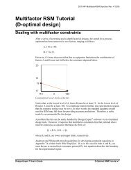
<strong>Multifactor</strong> <strong>RSM</strong> <strong>Tutorial</strong><br />
(<strong>Part</strong> 2 – <strong>Optimization</strong>)<br />
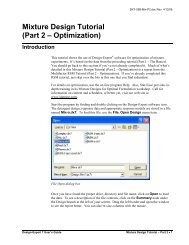
Introduction<br />
<strong>DX7</strong>1-04D-<strong>Multifactor</strong><strong>RSM</strong>-P2.docRev. 1/1/07<br />
This tutorial shows the use of Design-Expert software for optimization experiments. It's<br />
based on the data from the <strong>Multifactor</strong> <strong>RSM</strong> <strong>Tutorial</strong> <strong>Part</strong> 1. You should go back to this<br />
section if you've not already completed it.<br />
For details on optimization, see the on-line program help. Also, Stat-Ease provides indepth<br />
training in its Response Surface Methods for Process <strong>Optimization</strong> workshop.<br />
Call or visit our web site for <strong>info</strong>rmation on content and schedules.<br />
In this section, you will work with predictive models for two responses, yield and<br />
activity, as a function of three factors: time, temperature and catalyst. These models are<br />
based on results from a central composite design (CCD) on a chemical reaction.<br />
Start the program by finding and double clicking on the Design-Expert icon.<br />
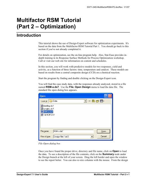
You will find the case study data, with the responses already analyzed, stored in a file<br />
named <strong>RSM</strong>-a.dx7. Use the File, Open Design menu to load the data file. The<br />
standard file open dialog box appears.<br />
File Open dialog box<br />
Once you have found the proper drive, directory and file name, click on Open to load<br />
the data. To see a description of the file contents, click on the Summary node under<br />
the Design branch at the left of your screen. Drag the left border and open the window<br />
to see the report better. You can also re-size columns with the mouse. From the design<br />
Design-Expert 7.1 User’s Guide <strong>Multifactor</strong> <strong>RSM</strong> <strong>Tutorial</strong> – <strong>Part</strong> 2 • 1
status screen you can see that we modeled conversion with a quadratic model and<br />
activity with a linear model.<br />
Design summary<br />
Numerical <strong>Optimization</strong><br />
Design-Expert software’s numerical optimization will maximize, minimize or target:<br />
• A single response<br />
• A single response, subject to upper and/or lower boundaries on other<br />
responses<br />
• Combinations of two or more responses.<br />
We will lead you through the latter case: a multiple response optimization. Under the<br />
<strong>Optimization</strong> branch of the program, click on the Numerical node to start the process.<br />
Setting numeric optimization criteria<br />
2 • <strong>Multifactor</strong> <strong>RSM</strong> <strong>Tutorial</strong> – <strong>Part</strong> 2 Design-Expert 7.1 User’s Guide
Setting the <strong>Optimization</strong> Criteria<br />
<strong>DX7</strong>1-04D-<strong>Multifactor</strong><strong>RSM</strong>-P2.docRev. 1/1/07<br />
Design-Expert allows you to set criteria for all variables, including factors and<br />
propagation of error (POE). (We will get to POE later.) To be safe, the program sets the<br />
factor ranges to the actual levels (plus one to minus one in coded values). The limits for<br />
the responses default to the observed extremes. In this case, you should leave the<br />
settings for time, temperature and catalyst factors alone, but you will need to make some<br />
changes to the response criteria.<br />
Now you get to the crucial phase of numerical optimization: assignment of<br />
“<strong>Optimization</strong> Parameters.” The program uses five possibilities for a “Goal” to<br />
construct desirability indices (di):<br />
• Maximize,<br />
• Minimize,<br />
• Target->,<br />
• In range,<br />
• Equal to -> (factors only).<br />
Desirabilities range from zero to one for any given response. The program combines the<br />
individual desirabilities into a single number and then searches for the greatest overall<br />
desirability. A value of one represents the ideal case. A zero indicates that one or more<br />
responses fall outside desirable limits. Design-Expert uses an optimization method<br />
developed by Derringer and Suich, described by Myers and Montgomery in Response<br />
Surface Methodology, John Wiley and Sons, New York (available from Stat-Ease).<br />
For this tutorial case study, assume that you need to increase conversion. Click on<br />
Conversion and set its Goal at maximize. Set the Lower and Upper Limits to 80,<br />
the lowest acceptable value, and 100, the theoretical high; respectively.<br />
Conversion criteria settings<br />
You must provide both these thresholds to get the desirability equation to work properly.<br />
By default they will be set at the observed response range, in this case 51 to 97. By<br />
Design-Expert 7.1 User’s Guide <strong>Multifactor</strong> <strong>RSM</strong> <strong>Tutorial</strong> – <strong>Part</strong> 2 • 3
increasing the upper end for desirability to 100, we put in a ‘stretch’ for the<br />
maximization goal. Otherwise we may come up short of the potential optimum.<br />
Now click on the second response, Activity. Set its Goal to target-> of 63. Enter<br />
Limits for Lower and Upper at 60 and 66; respectively. These limits indicate that it<br />
is most desirable to achieve the targeted value of 63, but values in the range of 60-66 are<br />
acceptable. Values outside that range are not acceptable.<br />
Activity criteria settings<br />
These settings create the following desirability functions:<br />
1. Conversion:<br />
• if less than 80%, then desirability (di) equals zero<br />
• from 80 to 100%, di ramps up from zero to one<br />
• if over 100%, then di equals one<br />
2. Activity:<br />
• if less than 60, then di equals zero<br />
• from 60 to 63, di ramps up from zero to one<br />
• from 63 to 66, di ramps back down to zero<br />
• if greater than 66, then di equals zero<br />
Do not forget that at your fingertips you will find advice on using sophisticated features<br />
of Design-Expert software: Press the button for Screen Tips on Numerical<br />
<strong>Optimization</strong>.<br />
4 • <strong>Multifactor</strong> <strong>RSM</strong> <strong>Tutorial</strong> – <strong>Part</strong> 2 Design-Expert 7.1 User’s Guide
Screen tips<br />
<strong>DX7</strong>1-04D-<strong>Multifactor</strong><strong>RSM</strong>-P2.docRev. 1/1/07<br />
Close out Screen Tips by pressing X at the upper-right corner of its screen.<br />
Changing Desirability Weights and the (Relative) Importance of Variables<br />
The user can select additional parameters, called “weights”, for each response. Weights<br />
give added emphasis to upper or lower bounds or emphasize a target value. With a<br />
weight of 1, the di will vary from 0 to 1 in linear fashion. Weights greater than 1<br />
(maximum weight is 10) give more emphasis to the goal. Weights less than 1 (minimum<br />
weight is 0.1) give less emphasis to the goal. Weights can be quickly changed by<br />
‘grabbing’ (via left mouse-click and drag) the handles (the squares ▫) on the desirability<br />
ramps. Try pulling the one on the left down and the right one up as shown below.<br />
Weights change by grabbing handles with mouse<br />
This might reflect a situation where your customer says they want the targeted value<br />
(63), but if it must be missed due to a trade-off necessary for other specifications, it<br />
would be better to error on the high side. Before moving on from here, re-enter the<br />
Lower and Upper Weights at their default values of 1 and 1; respectively. This will<br />
straighten them out to the original ‘tent’ shape (�).<br />
Design-Expert 7.1 User’s Guide <strong>Multifactor</strong> <strong>RSM</strong> <strong>Tutorial</strong> – <strong>Part</strong> 2 • 5
“Importance” is a tool for changing the relative priorities for achieving the goals you<br />
establish for some or all of the variables. If you want to emphasize one over the rest, set<br />
its importance higher. Design-Expert offers five levels of importance ranging from 1<br />
plus (+) to 5 plus (+++++). For this study, leave the Importance field at +++, a<br />
medium setting. By leaving all importance criteria at their default, none of the goals will<br />
be favored over any other.<br />
For an in-depth explanation of the construction of the desirability function, and formulas<br />
for the weights and importance, select Help off the main menu. Then go to Contents<br />
and select <strong>Optimization</strong>. Branch down to the topic of Importance as shown on the<br />
screen-shot below. From there you can open various topics and look for the details you<br />
need.<br />
Details on the optimization criterion “importance” found in program Help<br />
When you are done looking at Help, close it out by pressing X at the upper-right corner<br />
of the screen. Then, click the Options button to see how you gain control over how the<br />
numerical optimization will be performed. For example, you can change the number of<br />
cycles (searches) per optimization. If you have a very complex combination of response<br />
surfaces, increasing the number of cycles will give you more opportunities to find the<br />
optimal solution. The Duplicate solution filter establishes the epsilon (minimum<br />
difference) for eliminating essentially identical solutions. The Simplex Fraction<br />
specifies how big the initial steps will be relative to the factor ranges. (The word<br />
“simplex” relates to the geometry of the search. For two factors the simplex is an<br />
equilateral triangle. By stepping through the three corners the program figures out the<br />
path of steepest ascent. For more detail, go to Help and search on “numerical search<br />
algorithm.”)<br />
6 • <strong>Multifactor</strong> <strong>RSM</strong> <strong>Tutorial</strong> – <strong>Part</strong> 2 Design-Expert 7.1 User’s Guide
Running the optimization<br />
<strong>DX7</strong>1-04D-<strong>Multifactor</strong><strong>RSM</strong>-P2.docRev. 1/1/07<br />
Another optimization option is to not use random starting points, but rather those in the<br />
design itself. However, these will be limited to 100 unless you change this default.<br />
Leave this and all other options at their default levels shown below. (PS. This screen<br />
shot shows underlined letters that show Alt keys for jumping to fields via keystrokes<br />
versus mousing.)<br />
<strong>Optimization</strong> Options dialog box<br />
Start the optimization by clicking on the Solutions icon.<br />
Numerical <strong>Optimization</strong> Report on Solutions (Your results may differ)<br />
The program randomly picks a set of conditions from which to start its search for<br />
desirable results. Multiple cycles improve the odds of finding multiple local optimums,<br />
Design-Expert 7.1 User’s Guide <strong>Multifactor</strong> <strong>RSM</strong> <strong>Tutorial</strong> – <strong>Part</strong> 2 • 7
some of which will be higher in desirability than others. After grinding through 39<br />
cycles of optimization (30 chosen at random, plus 9 design points found within the<br />
factorial region of the central composite design), Design-Expert sorts the results for you<br />
in tabular form. Due to the random starting conditions, your results are likely to be<br />
slightly different from those in the report shown here. Note that the last solution falls<br />
short of the first for conversion. There may be some duplicates in between. These<br />
passed through the filter discussed earlier. If you want to adjust the filter, go to the<br />
Options button and change the Duplicate Solutions Filter. If you move the Filter bar to<br />
the right you will decrease the number of solutions shown. Likewise, moving the bar to<br />
the left increases the number of solutions.<br />
The Solutions Tool provides three views of the same optimization. (Drag the tool to a<br />
convenient location on the screen.) Click on the Solutions Tool view option Ramps.<br />
Ramps report on numerical optimization<br />
The ramp display combines the individual graphs for easier interpretation. The dot on<br />
each ramp reflects the factor setting or response prediction for that solution. The height<br />
of the dot shows how desirable it is. Press the different solution buttons (1, 2, 3,…) and<br />
watch the dots. They may move only very slightly from one solution to the next.<br />
However, if you look closely at temperature, you should find two distinct optimums, the<br />
first few near 90 degrees and further down the solution list, others near 80 degrees.<br />
(You may see slight differences in the results due to variations in approach from the<br />
various random starting points.) For example, click the last solution on your screen.<br />
Does it look something like the one below?<br />
8 • <strong>Multifactor</strong> <strong>RSM</strong> <strong>Tutorial</strong> – <strong>Part</strong> 2 Design-Expert 7.1 User’s Guide
<strong>DX7</strong>1-04D-<strong>Multifactor</strong><strong>RSM</strong>-P2.docRev. 1/1/07<br />
Second optimum at lower temperature, but conversion drops, so it is inferior<br />
If your search also uncovered this local optimum, you will note that conversion falls off,<br />
thus making it less desirable than the option for higher temperature.<br />
Select the Bar Graph view.<br />
Solution to multiple response optimization - desirability bar graph<br />
The bar graph shows how well each variable satisfied the criteria: values near one are<br />
good.<br />
Design-Expert 7.1 User’s Guide <strong>Multifactor</strong> <strong>RSM</strong> <strong>Tutorial</strong> – <strong>Part</strong> 2 • 9
<strong>Optimization</strong> Graphs<br />
Press Graphs to view a contour graph of overall desirability. Click Solutions button<br />
1. Then go to the Factors Tool control and right-click on C:Catalyst. Make it the<br />
X2 axis. Temperature then becomes a constant factor at 90 degrees.<br />
Desirability graph (after changing X2 axis to factor C)<br />
The screen shot above came from a graph done with graduated colors – cool blue for<br />
lower desirability and warm yellow for higher. If you just completed part 1 of this<br />
tutorial, your graph came up in only one color. This can be easily fixed by right-clicking<br />
over the graph and selecting Graph Preferences.<br />
Graph preferences via right-click menu – Selecting graduated (color) shading<br />
Click the Graphs 2 tab and make sure the Contour graph shading option is set at<br />
Graduated shading. Then press OK and see what you get.<br />
Design-Expert software sets a flag at the optimal point. To view the responses<br />
associated with the desirability, select the desired Response from the drop down list.<br />
Take a look at the plot for Conversion.<br />
10 • <strong>Multifactor</strong> <strong>RSM</strong> <strong>Tutorial</strong> – <strong>Part</strong> 2 Design-Expert 7.1 User’s Guide
Conversion contour plot (with optimum flagged)<br />
<strong>DX7</strong>1-04D-<strong>Multifactor</strong><strong>RSM</strong>-P2.docRev. 1/1/07<br />
The colors are neat, but what if you must print the graphs in black and white? This can<br />
be easily fixed by right-clicking over the graph and selecting Graph Preferences.<br />
Click the Graphs 2 tab and set the Contour graph shading option to Plain<br />
background.<br />
Graph preferences set to plain background<br />
While you’re at preferences, go to Graphs 1 tab and click Show 2D graph grid<br />
lines.<br />
Show grid lines option<br />
Finally, to make the graph really plain, go to the Fonts & Colors tab, choose Contour<br />
Background, click Edit Color and select white off the grid and press OK.<br />
Design-Expert 7.1 User’s Guide <strong>Multifactor</strong> <strong>RSM</strong> <strong>Tutorial</strong> – <strong>Part</strong> 2 • 11
Graph changed to black and white with grid lines<br />
There are many other options on this and other tabs for Graph preferences. Look them<br />
over if you like and then press OK to see what the options specified by this tutorial do<br />
for your contour plot. The grid lines help for locating the optimum, but for a more<br />
precise locator right-click on the flag and Toggle size to see the coordinates, plus lots<br />
of other detail on the predicted outcome.<br />
Flag size toggled to see more detail about optimum conversion<br />
By going back to Toggle size, you can change it back to the smaller flag. If you like,<br />
look at the optimal activity response as well.<br />
To look at the desirability surface in three dimensions, click again on Response and<br />
choose Desirability. Then select View, 3D Surface from the main menu. Then to get<br />
the view shown below, go to the Rotation tool and change the horizontal control h to<br />
170 and click on the graph. What a spectacular view!<br />
12 • <strong>Multifactor</strong> <strong>RSM</strong> <strong>Tutorial</strong> – <strong>Part</strong> 2 Design-Expert 7.1 User’s Guide
3D desirability plot<br />
<strong>DX7</strong>1-04D-<strong>Multifactor</strong><strong>RSM</strong>-P2.docRev. 1/1/07<br />
Now you can see that there’s a ridge where desirability can be maintained at a high level<br />
over a range of catalyst levels. In other words the solution is relatively robust to factor<br />
C. Go to the Factors Tool and move the slide bar on the B: Temperature. How does this<br />
affect desirability? If you have a color printer attached, make a hard copy by doing a<br />
File, Print. For black and white printing, right-click back to Graph preferences and<br />
on the Graphs 2 tab change the 3D graph drawing method option to Wire frame.<br />
3D graph changed to wire frame (for black and white printing)<br />
Press OK and see what you get. (To make the graph really plain (not done here), go to<br />
the Fonts & Colors tab, choose 3D Contour Background, click Edit Colors and select<br />
white off the grid.)<br />
Design-Expert 7.1 User’s Guide <strong>Multifactor</strong> <strong>RSM</strong> <strong>Tutorial</strong> – <strong>Part</strong> 2 • 13
Wire frame view of 3D desirability graph at high resolution<br />
One way or another please show your colleagues what Design-Expert software will do<br />
for pointing out most desirable combinations of process factors. (We’d like that!) The<br />
best way to show what you’ve got is not on paper, but rather by demonstrating it on your<br />
computer screen or with the output projected for a larger audience. In this case, you’d<br />
best shift back to the default colors and other display schemes. Do this by right-clicking<br />
and selecting Graph Preferences and pressing the Default buttons for the Graphs<br />
1, Graphs 2 and Fonts and Colors (Colors side only).<br />
Before moving on to graphical optimization, here is a postscript on the chromatic<br />
shading options offered in the Graphs 2 dialog box – a very esoteric feature that you<br />
may be wondering about. For your <strong>info</strong>rmation, monochromatic (“mono”) shading<br />
comes out flat like a gray scale, only instead of moving from black to white it changes<br />
from one color to another – the end colors are brighter and the middle ones darker.<br />
Dichromatic (“di”) shading improves the appearance by using a midpoint color that has<br />
the maximum RGB values of both end colors. However, in order to get the full range of<br />
colors, you have to use a completely different third color for the midpoint, which is what<br />
trichromatic (“tri”) shading does. The particular colors used (shading for Low, Middle,<br />
and High) can be selected from the Fonts & Colors tab under Colors (scroll down to see<br />
them). Feel free to mess around with these color options at this point, but if you are<br />
pressed for time, move on!<br />
14 • <strong>Multifactor</strong> <strong>RSM</strong> <strong>Tutorial</strong> – <strong>Part</strong> 2 Design-Expert 7.1 User’s Guide
Graphical <strong>Optimization</strong><br />
<strong>DX7</strong>1-04D-<strong>Multifactor</strong><strong>RSM</strong>-P2.docRev. 1/1/07<br />
When you generated the numerical optimization, you found an area of satisfactory<br />
solutions at a temperature of 90 degrees. To see a broader operating window, click on<br />
the Graphical node. The requirements are essentially the same as in the numerical<br />
optimization:<br />
• 80 < Conversion<br />
• 60 < Activity < 66<br />
For the first response – Conversion, (if not already entered) type in 80 for the Lower<br />
Limit. You do not need to enter a high limit for the graphical optimization to work.<br />
Graphical optimization: Conversion criteria<br />
Click on the response of Activity. If not already entered, type in 60 for the Lower<br />
Limit and 66 for the Upper Limit.<br />
Activity limits<br />
Design-Expert 7.1 User’s Guide <strong>Multifactor</strong> <strong>RSM</strong> <strong>Tutorial</strong> – <strong>Part</strong> 2 • 15
Then click on the Graphs button to produce the “overlay” plot. Notice that regions not<br />
meeting your specifications are shaded out, leaving (hopefully!) an operating window or<br />
“sweet spot.” (If you still see the grid lines you added earlier, right-click over the graph,<br />
select Graph Preferences, go to Graphs 1 tab and click the check mark off Show grid<br />
lines. These just clutter up the graph.)<br />
Now go to the Factors Tool control and right click on C:Catalyst. Make it the X2<br />
axis. Temperature then becomes a constant factor at 90 degrees as before for Solution<br />
1.<br />
Overlay plot<br />
Notice that the flag remains planted at the optimum. That’s handy! This display by<br />
Design-Expert may not look as fancy as the 3D of desirability but it can be very useful<br />
to show windows of operability where requirements simultaneously meet the critical<br />
properties. The shaded areas on the graphical optimization plot do not meet the<br />
selection criteria. The clear “window” shows where you can set the factors to satisfy the<br />
requirements on both responses. The lines that mark the high or low boundaries on the<br />
responses can be identified via a mouse-click. Notice that the contour and its label<br />
change color for easy identification.<br />
Let’s say that someone wonders whether the 80 minimum for conversion can be<br />
increased. What will this do to the operation window? Find out by dragging the 80<br />
conversion contour until it reaches a value of 90. Then click on the Activity 60 contour<br />
to see it more easily in the highlighted color.<br />
16 • <strong>Multifactor</strong> <strong>RSM</strong> <strong>Tutorial</strong> – <strong>Part</strong> 2 Design-Expert 7.1 User’s Guide
Changing the specification on conversion to 90 minimum<br />
<strong>DX7</strong>1-04D-<strong>Multifactor</strong><strong>RSM</strong>-P2.docRev. 1/1/07<br />
Caution: Having changed the criteria, the flagged optimum is no longer valid. To get it<br />
right you would have to go back to the Numerical optimization option and enter any new<br />
response criteria there.<br />
It appears that the more ambitious goal of 90 percent conversion is feasible. This change<br />
in requirements would make the lower activity specification superfluous.<br />
Graphical optimization works great for two factors, but as the factors increase, it<br />
becomes more and more tedious. You will find solutions much more quickly by using<br />
the numerical optimization feature. Then return to the graphical optimization and<br />
produce outputs for presentation purposes.<br />
Response Prediction at the Optimum<br />
Save the Data to a File<br />
Click on the Point Prediction node (lower left on your screen). Notice how it now<br />
defaults to the first solution. Then be thankful that the Design-Expert programmers<br />
thought of this, because it saves you the trouble of dialing it up on the Factors Tool.<br />
Point prediction set to solution #1<br />
Now that you’ve invested all this time into setting up the optimization for this design, it<br />
would be prudent to save your work. Click on the File menu item and select Save As.<br />
Design-Expert 7.1 User’s Guide <strong>Multifactor</strong> <strong>RSM</strong> <strong>Tutorial</strong> – <strong>Part</strong> 2 • 17
Final Comments<br />
Save As selection<br />
You can then specify the File name (we suggest tut-<strong>RSM</strong>-opt) to Save as type *.dx7”<br />
in the Data folder for Design-Expert (or wherever you want to Save in).<br />
File Save As dialog box<br />
You will need this file in <strong>Part</strong> 3 of this series of tutorials.<br />
We feel that numerical optimization provides powerful insights when combined with<br />
graphical analysis. Numerical optimization becomes essential when you investigate<br />
many factors with many responses. However, computerized optimization will not work<br />
very well in the absence of subject matter knowledge. For example, a naive user may<br />
define impossible optimization criteria. The result will be zero desirability everywhere!<br />
To avoid this, try setting broad acceptable ranges. Narrow them down as you gain<br />
knowledge about how changing factor levels affect the responses. Often, you will need<br />
to make more than one pass to find the “best” factor levels to satisfy constraints on<br />
several responses simultaneously.<br />
This Response Surface optimization tutorial completes the basic introduction to doing<br />
<strong>RSM</strong> with Design-Expert software. Move on to the next tutorial on advanced topics for<br />
multifactor <strong>RSM</strong> for more detail on what the software can do. If you want to learn more<br />
about the response surface methods (not the software per se), attend the Stat-Ease<br />
workshop Response Surface Methods for Process <strong>Optimization</strong>.<br />
We appreciate your questions and comments on Design-Expert software. Call us, send<br />
an annotated fax of output, write us a letter or send us an e-mail. You will find our<br />
contact <strong>info</strong>rmation and email links at www.statease.com.<br />
18 • <strong>Multifactor</strong> <strong>RSM</strong> <strong>Tutorial</strong> – <strong>Part</strong> 2 Design-Expert 7.1 User’s Guide