An Introduction to Genetic Algorithms - Boente

Chapter 2: Genetic Algorithms in Problem Solving
An initial population of 50 weight vectors was chosen randomly, with each weight being between ‘.0 and +
1.0. Montana and Davis tried a number of different genetic operators in various experiments. The mutation
and crossover operators they used for their comparison of the GA with back−propagation are illustrated in
Figure 2.18 and Figure 2.19. The mutation operator selects n non−input units and, for each incoming link to
those units, adds a random value between ‘.0 and + 1.0 to the weight on the link. The crossover operator
takes two parent weight vectors and, for each non−input unit in the offspring vector, selects one of the parents
at random and copies the weights on the incoming links from that parent to the offspring. Notice that only one
offspring is created.
The performance of a GA using these operators was compared with the performance of a back−propagation
algorithm. The GA had a population of 50 weight vectors, and a rank−selection method was used. The GA
was allowed to run for 200 generations (i.e., 10,000 network evaluations). The back−propagation algorithm
was allowed to run for 5000 iterations, where one iteration is a complete epoch (a complete pass through the
training data). Montana and Davis reasoned that two network evaluations
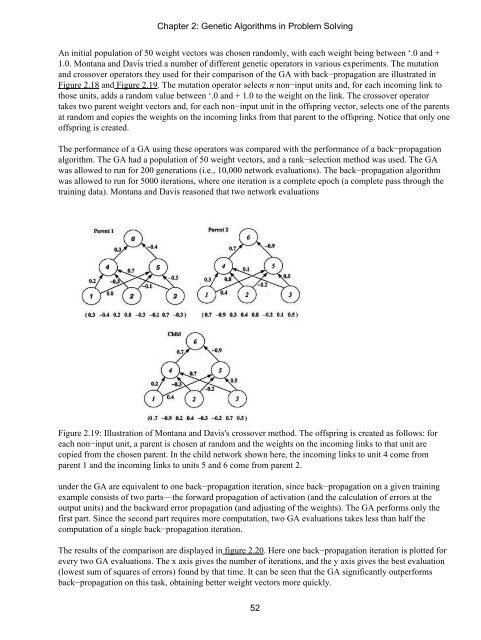
Figure 2.19: Illustration of Montana and Davis's crossover method. The offspring is created as follows: for
each non−input unit, a parent is chosen at random and the weights on the incoming links to that unit are
copied from the chosen parent. In the child network shown here, the incoming links to unit 4 come from
parent 1 and the incoming links to units 5 and 6 come from parent 2.
under the GA are equivalent to one back−propagation iteration, since back−propagation on a given training
example consists of two parts—the forward propagation of activation (and the calculation of errors at the
output units) and the backward error propagation (and adjusting of the weights). The GA performs only the
first part. Since the second part requires more computation, two GA evaluations takes less than half the
computation of a single back−propagation iteration.
The results of the comparison are displayed in figure 2.20. Here one back−propagation iteration is plotted for
every two GA evaluations. The x axis gives the number of iterations, and the y axis gives the best evaluation
(lowest sum of squares of errors) found by that time. It can be seen that the GA significantly outperforms
back−propagation on this task, obtaining better weight vectors more quickly.
52