An Introduction to Determining Optimum Quadrat Size and Shape
An Introduction to Determining Optimum Quadrat Size and Shape
An Introduction to Determining Optimum Quadrat Size and Shape

Create successful ePaper yourself
Turn your PDF publications into a flip-book with our unique Google optimized e-Paper software.
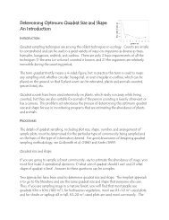
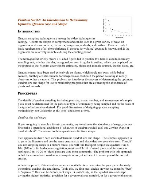
Problem Set #2: <strong>An</strong> <strong>Introduction</strong> <strong>to</strong> <strong>Determining</strong><br />
<strong>Optimum</strong> <strong>Quadrat</strong> <strong>Size</strong> <strong>and</strong> <strong>Shape</strong><br />
INTRODUCTION<br />
<strong>Quadrat</strong> sampling techniques are among the oldest techniques in<br />
ecology. Counts are simple <strong>to</strong> comprehend <strong>and</strong> can be used in a great variety of ways on<br />
organisms as diverse as trees, barnacles, kangaroos, seabirds, <strong>and</strong> caribou. There are only 2<br />
basic requirements of all the techniques: 1) the area (or volume) counted is known, <strong>and</strong> 2) the<br />
organisms are relatively immobile during the counting period.<br />
The term quadrat strictly means a 4-sided figure, but in practice this term is used <strong>to</strong> mean any<br />
sampling unit, whether circular, hexagonal, or even irregular in outline, which can be placed on<br />
the ground so that % plant cover can be estimated, plants <strong>and</strong> animals counted, species listed, etc.<br />
<strong>Quadrat</strong> counts have been used extensively on plants, which rarely run away while being<br />
counted, but they are also suitable for kangaroos or caribou if the person counting is keenly<br />
observant or has a camera. This problem set introduces the process of determining the optimum<br />
quadrat size <strong>and</strong> shape for use in moni<strong>to</strong>ring programs that are estimating the abundance of<br />
plants <strong>and</strong> animals.<br />
PROCEDURES<br />
The details of quadrat sampling, including plot size, shape, number, <strong>and</strong> arrangement of sample<br />
plots, must be determined for the particular type of community being sampled <strong>and</strong> on the basis of<br />
the type of information desired. For good discussions of designing quadrat sampling<br />
methodology, see Goldsmith et al. (1986) <strong>and</strong> Krebs (1999).<br />
<strong>Quadrat</strong> size <strong>and</strong> shape<br />
If you are going <strong>to</strong> sample a forest community, say <strong>to</strong> estimate the abundance of snags, you must<br />
first make 2 operational decisions: 1) what size of quadrat should I use? <strong>and</strong> 2) what shape of<br />
quadrat is best? The answer <strong>to</strong> these questions is far from simple.<br />
Two approaches have been used <strong>to</strong> determine quadrat size <strong>and</strong> shape. The simplest approach is<br />
<strong>to</strong> go <strong>to</strong> the literature <strong>and</strong> use the same quadrat size <strong>and</strong> shape that everyone else uses. Thus, if<br />
you are sampling snags in a mature forest, you will find that most people use quadrats 10m x<br />
10m (100 m 2 ); for herbaceous vegetation, most use 0.1-1.0 m 2 -sized plots; <strong>and</strong> for shrubs or<br />
saplings ≤3 m, 10-20 m 2 -sized plots are used most commonly. The problem with this approach<br />
is that the accumulated wisdom of ecologists is not yet sufficient <strong>to</strong> assure you of the correct<br />
answer.<br />
A better approach, if time <strong>and</strong> resources are available, is <strong>to</strong> determine for your particular study<br />
the optimal quadrat size <strong>and</strong> shape. To do this, we first must decide on what we mean by “best”<br />
or “optimal.” Best can be defined in 3 ways: 1) statistically, as that quadrat size <strong>and</strong> shape<br />
giving the highest statistical precision for a given <strong>to</strong>tal area sampled, or for a given <strong>to</strong>tal amount
of time or money; 2) ecologically, as that quadrat size <strong>and</strong> shape that are most efficient <strong>to</strong> answer<br />
the question being asked; <strong>and</strong> 3) logistically, as that quadrat size <strong>and</strong> shape that are easiest <strong>to</strong><br />
establish in the field <strong>and</strong> use. Be wary of the logistical criterion, however, since in many<br />
ecological cases the easiest is rarely the best. If you are investigating questions of ecological<br />
scale, the processes you are studying will dictate quadrat size, but in most cases the statistical<br />
criterion <strong>and</strong> the ecological criterion are the same. In all these cases we define statistical<br />
precision as the lowest st<strong>and</strong>ard error of the mean <strong>and</strong> the arrowest confidence interval for the<br />
mean.<br />
In almost all cases we will encounter, we should determine the quadrat size <strong>and</strong> shape that will<br />
give us the highest statistical precision. How can we do this?<br />
Let’s consider the shape question first. There are 2 conflicting problems with shape. First, the<br />
edge effect is smallest in a circular quadrat, <strong>and</strong> largest in a rectangular one. The ratio of length<br />
of edge <strong>to</strong> the area inside a quadrat changes as follows:<br />
Circle < Square < Rectangle<br />
Edge effect is important because it leads <strong>to</strong> possible counting errors. A decision must be made<br />
every time an animal or plant is at the edge of a quadrat: Is this individual inside or outside the<br />
area <strong>to</strong> be counted? This decision is often biased by keen biologists who prefer <strong>to</strong> count an<br />
organism rather than ignore it. Edge effects thus often produce positive biases (i.e., the numbers<br />
of organisms counted within the quadrat are higher than they should be. This positive bias could<br />
obviously lead <strong>to</strong> a population estimate that is <strong>to</strong>o high). Proportionally, the more edge your plot<br />
has the more positive bias results. The general significance of possible errors of counting at the<br />
edge of a quadrat cannot be quantified because it is organism- <strong>and</strong> habitat-specific. It can,<br />
however, be reduced by training. If edge effects are a significant source of error, you should<br />
choose a quadrat shape with less edge/area. But how do you know you might have an edge<br />
effect problem? Figure 1 illustrates 1 way of recognizing an edge effect problem. Note that<br />
there is no reason <strong>to</strong> expect any bias in mean abundance estimated from a variety of quadrat sizes<br />
<strong>and</strong> shapes. If there is no edge effect bias, we expect in an ideal world <strong>to</strong> get the same mean<br />
value regardless of the size or shape of the quadrats used, if the mean is expressed in the same<br />
units of area. This is important <strong>to</strong> remember: <strong>Quadrat</strong> size <strong>and</strong> shape are not about biased<br />
abundance estimates but are about narrower confidence limits. If you find a relationship like that<br />
in Figure 1 in data set you are working on, you should immediately disqualify the smallest<br />
quadrat size from consideration <strong>to</strong> avoid bias from the edge effect.<br />
2
Figure 1. Edge effect bias in small quadrats. The estimated mean dry weight of grass (per 0.25<br />
m 2 ) is much higher in quadrat size 1 (0.016 m 2 ) than in all other quadrat sizes. This suggests an<br />
overestimation bias due <strong>to</strong> edge effects, <strong>and</strong> that quadrat size 1 should not be used <strong>to</strong> estimate<br />
abundance of these grasses. The data are from Wiegert (1962).<br />
The second problem regarding quadrat shape is that nearly everyone has found that long, thin<br />
quadrats are better than circular or square ones of the same area. The reason for this is because<br />
of habitat heterogeneity. Long quadrats cross more patches <strong>and</strong> thus capture more of the habitat<br />
variability (something you want <strong>to</strong> do). Areas are never uniform, <strong>and</strong> organisms are usually<br />
distributed somewhat patchily within the overall sampling zone. Clapham (1932) counted the<br />
number of self-heal (Prunella vulgaris) plants in 1-m 2 quadrats of 2 shapes: 1m x 1m <strong>and</strong> 4m x<br />
0.25 m. He counted 16 quadrats <strong>and</strong> got these results:<br />
<strong>Quadrat</strong> size Mean Variance SE 95% CI<br />
1m x 1m 24 565.3 5.94 ±12.65<br />
4m x 0.25m 24 333.3 4.56 ±9.71<br />
Clearly in this situation, the rectangular quadrats are more efficient than square ones (i.e., the SE<br />
is lower <strong>and</strong> the CI is narrower). Given that only 2 shapes of quadrats were tried, we do not<br />
know if even longer, thinner quadrats might be still more efficient.<br />
Not all sampling data show this preference for long, thin quadrats, <strong>and</strong> for this reason each<br />
situation should be analyzed on its own. Table 1 shows data from basal area measurements on<br />
trees in a forest st<strong>and</strong> studied by Bormann (1953). The observed SD almost always falls as<br />
quadrat area increases. But if an equal <strong>to</strong>tal area is being sampled, the highest precision<br />
(=lowest SE) will be obtained by using 70 4m x 4m quadrats (Table 1). If, on the other h<strong>and</strong>, an<br />
equal number of quadrats were <strong>to</strong> be taken for each quadrat size, one would prefer the long, thin<br />
quadrat shape.<br />
3
Table 1. Effect of quadrat size on SD for measurements of basal area of trees in an oak-hickory<br />
forest in North Carolina. The data are from Bormann (1953).<br />
<strong>Quadrat</strong> size Observed SD<br />
(m) per 4 m 2<br />
Sample size a<br />
SE of the<br />
mean for<br />
sample size<br />
4 x 4 50.7 70 6.06<br />
4 x 10 47.3 28 8.94<br />
4 x 20 44.6 14 11.92<br />
4 x 70 41.3 4 20.65<br />
4 x 140 34.8 2 24.61<br />
a 2<br />
The number of quadrats of a given size needed <strong>to</strong> sample 1,120 m .<br />
Two methods are available for choosing the best quadrat size statistically. Wiegert (1962)<br />
proposed a general method that can be used <strong>to</strong> determine optimal size or shape. Hendricks<br />
(1956) proposed a more restrictive method for estimating optimal size of quadrats. In both<br />
methods it is essential that data from all quadrats be st<strong>and</strong>ardized <strong>to</strong> a single unit area—for<br />
example, per m 2 . This conversion is simple for means, SDs, <strong>and</strong> SEs: divide by the relative area.<br />
For example,<br />
Mean number per m 2 2<br />
Mean number per 0.25m<br />
=<br />
0.25<br />
SD per m 2 2<br />
SD per 4m<br />
=<br />
4<br />
For variances, the square of the conversion fac<strong>to</strong>r is used:<br />
Variance per m 2 =<br />
2<br />
Varianceper<br />
9 m<br />
2<br />
9<br />
For both Wiegert’s <strong>and</strong> Hendrick’s methods, you should st<strong>and</strong>ardize all data <strong>to</strong> a common base<br />
area before testing for optimal size or shape of quadrat. They both assume further that you have<br />
tested for <strong>and</strong> eliminated quadrat sizes that give an edge effect bias. We will only deal with<br />
Wiegert’s method here.<br />
Wiegert’s method<br />
Wiegert (1962) proposed that 2 fac<strong>to</strong>rs were of primary importance in deciding on optimal<br />
quadrat size or shape: relative variability <strong>and</strong> relative cost. In any field study, time or money<br />
would seem <strong>to</strong> be the limiting resource, <strong>and</strong> we must consider how <strong>to</strong> optimize with respect <strong>to</strong><br />
sampling time. We will assume that time = money, <strong>and</strong> in the formulas that follow, either unit<br />
may be used. Costs of sampling have 2 components (in a simple world anyway):<br />
C = C0 + Cx,<br />
4
where C = Total cost for 1 sample<br />
C0 = Fixed costs or overhead<br />
Cx = Cost for taking 1 sample quadrat of size x.<br />
Fixed costs involve the time spent walking or flying between sampling points <strong>and</strong> the time spent<br />
locating a r<strong>and</strong>om point for the quadrat; these costs may be trivial in an open grassl<strong>and</strong>; they can<br />
be enormous when sampling the ocean in a large ship. The cost for taking a single quadrat may<br />
or may not vary with the size of the quadrat. Consider a simple example from Wiegert (1962) of<br />
grass biomass in quadrats of different sizes:<br />
<strong>Quadrat</strong> size (area)<br />
1 3 4 12 16<br />
Fixed cost ($) 10 10 10 10 10<br />
Cost per sample ($) 2 6 8 24 32<br />
Total cost for 1 quadrat ($) 12 16 18 34 42<br />
Relative cost for 1 quadrat 1 1.33 1.50 2.83 3.50<br />
We need <strong>to</strong> balance these costs against the relative variability of samples taken with quadrats of<br />
different sizes:<br />
<strong>Quadrat</strong> size (area)<br />
1 3 4 12 16<br />
Observed variance per 0.25 m 2 0.97 0.24 0.32 0.14 0.15<br />
The operational rule is, Pick the quadrat size that minimizes the product of (Relative cost) x<br />
(Relative variability).<br />
In this example, we begin by disqualifying quadrat size 1 because it showed a strong edge effect<br />
bias (Figure 1). Figure 2 shows that the optimal quadrat size for grass in this particular study is<br />
3, although there is relatively little difference between the products for quadrats of size 3, 4, 12,<br />
<strong>and</strong> 16. In this case, the size 3 quadrat gives the maximum precision for the least cost.<br />
5
Figure 2. <strong>Determining</strong> the optimal quadrat size for sampling. The best quadrat size is that which<br />
gives the minimal value of the product of relative cost <strong>and</strong> relative variability, which is quadrat<br />
size 3 in this example. <strong>Quadrat</strong> size 1 is plotted here for illustration, even though this quadrat<br />
size is disqualified because of edge effects. Data here are dry weights of grasses in quadrats of<br />
variable size. Data are from Wiegert (1962).<br />
Let’s work through an example from start <strong>to</strong> finish. The data we are using comes from Pringle’s<br />
(1984) study of seaweed (Chondrus crispus) biomass. As you can see from Table 2, Pringle<br />
tried quadrats of several different sizes in a pilot study <strong>to</strong> assist him in selecting the most<br />
appropriate-sized quadrat.<br />
Table 2. Data <strong>to</strong> determine optimal quadrat size for biomass estimates of the seaweed, Chondrus<br />
crispus (from Pringle 1984).<br />
<strong>Quadrat</strong> size<br />
(m) Sample size a<br />
Mean<br />
biomass b<br />
(g) SD b<br />
SE of the<br />
mean b<br />
Time <strong>to</strong> take<br />
1 sample<br />
(min)<br />
0.5 x 0.5 79 1524 1022 115 6.7<br />
1 x 1 20 1314 963 215 12.0<br />
1.25 x 1.25 13 1037 605 168 13.2<br />
1.5 x 1.5 9 1116 588 196 11.4<br />
1.73 x 1.73 6 2021 800 327 33.0<br />
2 x 2 5 1099 820 367 23.0<br />
a 2<br />
Sample sizes are approximately the number <strong>to</strong> make a <strong>to</strong>tal sampling area of 20 m .<br />
b 2<br />
All expressed per m .<br />
If we neglect any fixed costs <strong>and</strong> use the time <strong>to</strong> take 1 sample as the <strong>to</strong>tal cost, we can calculate<br />
the relative cost for each quadrat size as<br />
Relative cost =<br />
Time <strong>to</strong> take1sampleof<br />
a givensize<br />
Minimum time <strong>to</strong> take1sample<br />
In this case the minimum time = 6.7 minutes for the 0.5 x 0.5 quadrat (that shouldn’t be<br />
surprising). We can also express the variance (SD) 2 on a relative scale:<br />
6<br />
Equation 1
Relative variance =<br />
(SD)<br />
2<br />
(MinimumSD)<br />
2<br />
7<br />
Equation 2<br />
In this case, the minimum variance occurs for quadrats of 1.5 x 1.5 m. We obtain for these data:<br />
<strong>Quadrat</strong> size<br />
(m)<br />
Relative<br />
variance<br />
Relative<br />
cost<br />
Product of relative<br />
variance <strong>and</strong><br />
relative cost<br />
0.5 x 0.5 3.02 1.00 3.02<br />
1 x 1 2.68 1.79 4.80<br />
1.25 x 1.25 1.06 1.97 2.09<br />
1.5 x 1.5 1.00 1.70 1.70<br />
1.73 x 1.73 1.85 4.93 9.12<br />
2 x 2 1.94 3.43 6.65<br />
The operational rule is <strong>to</strong> pick the quadrat size with minimal product of cost x variance, <strong>and</strong> this<br />
is clearly the 1.5 x 1.5 m quadrat, which is the optimal quadrat size for this particular sampling<br />
area.<br />
There is a slight suggestion of a positive bias in the mean biomass estimates for the smallest<br />
quadrats, but this was not tested for by Pringle. In case you are wondering, the optimal quadrat<br />
shape could be decided in exactly the same way as quadrat size. Would there ever be a time<br />
when you might not want <strong>to</strong> determine optimum quadrat size <strong>and</strong> shape?<br />
Sampling plant <strong>and</strong> animal populations with quadrats is done for many different reasons, <strong>and</strong> it is<br />
important <strong>to</strong> ask when you might be advised <strong>to</strong> ignore the recommendations for quadrat size <strong>and</strong><br />
shape that arise from Wiegert’s method. There are 2 common situations when you may wish <strong>to</strong><br />
ignore these recommendations. In some cases you will wish <strong>to</strong> compare your data with older<br />
data gathered with a specific quadrat size <strong>and</strong> shape. Even if the older quadrat size <strong>and</strong> shape are<br />
inefficient, you may be advised, for comparative purposes, <strong>to</strong> continue using the old quadrat size<br />
<strong>and</strong> shape. In principle this is not required, as long as no bias is introduced by a change in<br />
quadrat size. But in practice, many biologists are more comfortable using the same quadrats as<br />
the earlier studies. This can become a more serious problem in a long-term moni<strong>to</strong>ring program<br />
in which a poor choice of quadrat size in the early stages could condemn the whole project <strong>to</strong><br />
wasting time <strong>and</strong> resources with inefficient sampling procedures.<br />
If you are sampling several habitats, sampling for many different species, <strong>and</strong>/or sampling over<br />
several seasons, you may find that these procedures result in a recommendation for a different<br />
size <strong>and</strong> shape of quadrat for each situation. It may be impossible <strong>to</strong> do this for logistical<br />
reasons, <strong>and</strong> thus you may have <strong>to</strong> compromise.
NOW YOU DO IT<br />
Exercise #1: A field plot was located in the subalpine zone of Glacier National Park, Montana<br />
<strong>and</strong> divided in<strong>to</strong> 16 quadrats of 1-m 2 . The numbers of queencup, Clin<strong>to</strong>nia uniflora, were<br />
counted in each quadrat with these results:<br />
3 0 5 1<br />
5 7 2 0<br />
3 2 0 7<br />
3 3 3 4<br />
Calculate the precision (i.e., SE of the mean <strong>and</strong> CI) of sampling this universe with 2 possible<br />
shapes of 4-m 2 quadrats: 2m x 2m <strong>and</strong> 4m x 1m.<br />
Exercise #2: Using the mapped population of a 17,860-m 2 (1.8 ha) st<strong>and</strong> of hardwoods in<br />
northern Minnesota provided, use Wiegert’s method <strong>to</strong> determine the optimum quadrat size <strong>to</strong><br />
determine the number of balsam fir trees (species #1 on the map). Table 3 contains the quadrat<br />
sizes you will compare, the required sample sizes for each quadrat size (yes, you will need <strong>to</strong><br />
sample at the intensity indicated), <strong>and</strong> the estimated time required <strong>to</strong> take 1 sample at each<br />
quadrat size (these numbers are provided <strong>and</strong> are mere guesses of the amount of time it would<br />
actually take <strong>to</strong> search a quadrat of each size for balsam fir trees). Notice that sample size is<br />
being held constant relative <strong>to</strong> the quadrat size so that each quadrat size is sampling the same<br />
area. We will discuss ways of determining sample sizes latter. You need <strong>to</strong> calculate the mean<br />
number of balsam fir trees, the SD, <strong>and</strong> the SE of the mean for each quadrat size. Record your<br />
data in Table 3. With these data, use Equations 1 <strong>and</strong> 2 <strong>to</strong> determine optimum quadrat size.<br />
Record your calculations in Table 4.<br />
Use the 3 quadrats provided on the overhead transparency. <strong>Quadrat</strong>s could be located r<strong>and</strong>omly<br />
using the 2 numbered axes placed along the edges of the sampling frame. As you can see, the<br />
axes divide the sampling frame in<strong>to</strong> cells. Using a r<strong>and</strong>om numbers table, you could ..select a<br />
pair of numbers (x <strong>and</strong> y) <strong>and</strong> use these numbers <strong>to</strong> place your quadrat on the map. Perhaps you<br />
would place the lower left corner of each quadrat on each r<strong>and</strong>omly-located point.<br />
8
Table 3. Optimal quadrat size for population estimates of balsam fir.<br />
<strong>Quadrat</strong> size<br />
(m)<br />
Sample size a<br />
Mean<br />
number of<br />
balsam fir b<br />
SD b<br />
SE of the<br />
mean b<br />
Time <strong>to</strong> take<br />
1 sample<br />
(min)<br />
10m x 10m 178 3<br />
25m x 25m 28 8<br />
50m x 50m 7 15<br />
a<br />
Sample sizes are approximately the number of quadrats <strong>to</strong> make a <strong>to</strong>tal sampling area of<br />
17,860m 2 .<br />
b 2<br />
All expressed per m .<br />
Table 4. Wiegert’s method <strong>to</strong> determine optimal quadrat size for counting balsam fir in a<br />
northern hardwood st<strong>and</strong>.<br />
<strong>Quadrat</strong> size Relative Relative Product of relative<br />
(m) variance cost variance <strong>and</strong><br />
relative cost<br />
10m x 10m<br />
25m x 25m<br />
50m x 50m<br />
SOME MORE TO THINK ABOUT<br />
1. What is the most optimum quadrat size <strong>to</strong> count balsam fir in this northern hardwood st<strong>and</strong>?<br />
2. How would you go about determining optimum quadrat shape? Work up an approach <strong>and</strong> do<br />
it. A couple of blank overhead transparencies are provided for your use. What is the most<br />
optimum quadrat shape <strong>to</strong> count balsam fir in this northern hardwood st<strong>and</strong>?<br />
ACKNOWLEDGEMENTS<br />
The bulk of this problem set was taken from Krebs (1999), particularly chapter 4.<br />
9
LITERATURE CITED<br />
Bormann, F.H. 1953. The statistical efficiency of sample plot size <strong>and</strong> shape in forest ecology.<br />
Ecology 34:474-487.<br />
Clapham, A. R. 1932. The form of the observational unit in quantitative ecology. Journal of<br />
Ecology 20:192-197.<br />
Goldsmith, F.B., C.M. Harrison, <strong>and</strong> A.J. Mor<strong>to</strong>n. 1986. Description <strong>and</strong> analysis of vegetation.<br />
Pages 437-524 in P.D. Moore <strong>and</strong> S.B. Chapman, edi<strong>to</strong>rs. Methods in plant ecology.<br />
Blackwell Scientific Publications, Oxford, Engl<strong>and</strong>.<br />
Krebs, C.J. 1999. Ecological methodology. Addison-Wesley Educational Publishers, Inc., Menlo<br />
Park, CA. 620 pp.<br />
Pringle, J.D. 1984. Efficiency estimates for various quadrat sizes used in benthic sampling.<br />
Canadian Journal of Fisheries <strong>and</strong> Aquatic Sciences 41:1485-1489.<br />
Wiegert, R.G. 1962. The selection of an optimum quadrat size for sampling the st<strong>and</strong>ing crop of<br />
grasses <strong>and</strong> forbs. Ecology 43:125-129.<br />
10