k - IFEN

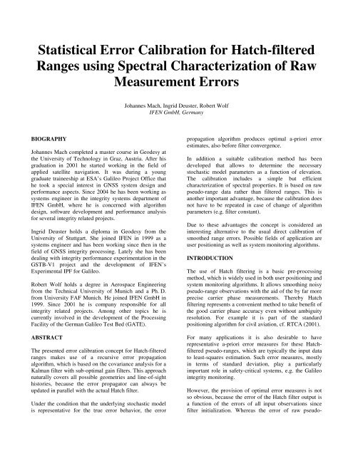
Statistical Error Calibration for Hatch-filtered
Ranges using Spectral Characterization of Raw
Measurement Errors
BIOGRAPHY
Johannes Mach completed a master course in Geodesy at
the University of Technology in Graz, Austria. After his
graduation in 2001 he started working in the field of
applied satellite navigation. It was during a young
graduate traineeship at ESA’s Galileo Project Office that
he took a special interest in GNSS system design and
performance aspects. Since 2004 he has been working as
systems engineer in the integrity systems department of
IFEN GmbH, where he is concerned with algorithm
design, software development and performance analysis
for several integrity related projects.
Ingrid Deuster holds a diploma in Geodesy from the
University of Stuttgart. She joined IFEN in 1999 as a
systems engineer and has been working since then in the
field of GNSS integrity processing. Lately she has been
dealing with integrity performance experimentation in the
GSTB-V1 project and the development of IFEN’s
Experimental IPF for Galileo.
Robert Wolf holds a degree in Aerospace Engineering
from the Technical University of Munich and a Ph. D.
from University FAF Munich. He joined IFEN GmbH in
1999. Since 2001 he is company responsible for all
integrity related projects. Among other topics he is
currently involved in the development of the Processing
Facility of the German Galileo Test Bed (GATE).
ABSTRACT
The presented error calibration concept for Hatch-filtered
ranges makes use of a recursive error propagation
algorithm, which is based on the covariance analysis for a
Kalman filter with sub-optimal gain filters. This approach
naturally covers all possible geometries and line-of-sight
histories, because the error propagator can always be
updated in parallel with the actual Hatch filter.
Under the condition that the underlying stochastic model
is representative for the true error behavior, the error
Johannes Mach, Ingrid Deuster, Robert Wolf
IFEN GmbH, Germany
propagation algorithm produces optimal a-priori error
estimates, also before filter convergence.
In addition a suitable calibration method has been
developed that allows to determine the necessary
stochastic model parameters as a function of elevation.
The calibration includes a simple but efficient
characterization of spectral properties. It is based on raw
pseudo-range data rather than filtered ranges. This is
another important advantage, because the calibration does
not have to be repeated in case of change of algorithm
parameters (e.g. filter constant).
Due to these advantages the concept is considered an
interesting alternative to the usual direct calibration of
smoothed range errors. Possible fields of application are
user positioning as well as system monitoring algorithms.
INTRODUCTION
The use of Hatch filtering is a basic pre-processing
method, which is widely used in both user positioning and
system monitoring algorithms. It allows smoothing noisy
pseudo-range observations with the aid of the by far more
precise carrier phase measurements. Thereby Hatch
filtering represents a convenient method to take benefit of
the good carrier phase accuracy even without ambiguity
resolution. For example it is part of the standard
positioning algorithm for civil aviation, cf. RTCA (2001).
For many applications it is also desirable to have
representative a-priori error measures for these Hatchfiltered
pseudo-ranges, which are typically the input data
to least-squares estimation. Such error measures, mostly
in terms of standard deviation, play a particularly
important role in safety-critical systems, e.g. the Galileo
integrity monitoring.
However, the provision of optimal error measures is not
so obvious, because the error of the Hatch filter output is
a function of the errors of all input observations since
filter initialization. Whereas the error of raw pseudo-

anges can usually be calibrated as an elevationdependent
function, the error of a smoothed range
depends on the entire history of the given line-of-sight,
including previous elevation angles, the filter time (time
elapsed since filter initialization) and data gaps.
This characteristic property of the Hatch filter makes
“direct calibration” of smoothed ranges quite difficult,
because in principle statistical calibration tables have to
be established with respect to both elevation and filter
time. However this requires an even larger amount of
archived data and the results are still not accurate, because
this approach does not account for data gaps and the exact
elevation history.
Therefore calibration is usually performed only with
respect to elevation and only for the smoothed range error
after filter convergence. This approach is feasible but
clearly not optimal, since lines-of-sight can be used only
after filter convergence and the elevation dependence has
to be conservative to cover all situations. For example, the
calibration for a low elevation has to cover the case of an
ascending satellite (even lower elevations in the past),
whereas the accuracy of a descending line-of-sight
(higher elevations in the past) might be significantly
better.
The algorithm proposed in this paper is able to overcome
the mentioned drawbacks by means of individual
covariance propagation for each line-of-sight, always in
parallel with the corresponding smoothing filter. Unlike
other concepts it is based on statistical calibration of raw
(unfiltered) pseudo-range errors, including its spectral
characterization in terms of auto-correlation.
The following sections describe the new error propagation
algorithm, a possible error model (still to be validated in
more detail) and a suitable calibration method.
THE COLOURED NOISE PROBLEM
The standard Hatch filter is defined by the following
recursive formula (cf. Hofmann-Wellenhof et al., 1998):
R ˆ
ˆ
) + w
w
k = ( 1−
wk
)( Rk−
1 + ϕ k −ϕ
k−1
k
with
⎧ 1/
k
= ⎨
⎩1/
T
flt
for k < T
for k ≥ T
Ri ˆ ...........smoothed pseudo-range (epoch i)
R ...........raw pseudo-range (epoch i)
i
ϕ ............carrier phase (epoch i)
i
flt
flt
k
R
k
w i ...........weight factor (epoch i)
T ..........filter constant (e.g. 300 seconds)
flt
The above formula shows that at any epoch the smoothed
range is a linear combination of the smoothed range of the
previous epoch as well as “raw” pseudo-range and carrier
phase observations. Therefore it appears possible to use
simple standard covariance propagation for linear
functions to propagate the variance. This would indeed be
possible for “white” noise errors. However, pseudo-range
errors usually are affected by time-correlated “coloured”
noise, which is mainly caused by multi-path effects. As a
consequence the new observation in general is correlated
with the smoothed range of the previous epoch. This
correlation somehow has to be taken into account,
otherwise results will be wrong (usually optimistic).
One option would be to use the explicit (non-recursive)
expression of the smoothed range as linear function of
raw observations only.
∑ − k 1
i=
0
Rˆ = w ( R + ϕ −ϕ
k
k,
i
k −i
with ∏ − i
w
k,
i
= w
1
k−i
j=
0
k
( 1−
w
k −i
k−
j
In that case one has only to deal with correlations between
raw measurements, which can be derived from a model.
Unfortunately the Hatch filter has an infinite impulse
response, which means that the above sum can become
very long (theoretically infinite), at least if exact
computation is desired (without truncation). Due to the
resulting large matrix multiplications this approach is
very inconvenient and rather unsuitable for practical
processing with many lines-of-sight.
Therefore we are considering a recursive algorithm,
which is presented in the following section. As explained
above, for a recursive algorithm it is always necessary to
model the correlation between raw observations and
smoothed ones, and this is what represents the main
difficulty in this context.
ERROR PROPAGATION ALGORITHM
Kalman-like formulation of Hatch filter
The Hatch filter output is computed as a weighted average
of the smoothed pseudo-range of the previous epoch,
propagated to the current epoch using phase observations,
and the current raw pseudo-range. This is equivalent to a
Kalman filter recursion, with the important difference that
the weight of the new observation is pre-determined and
)
)

not computed from a stochastic model. In fact, the
following matrix notation of the Hatch filter
⎡Rˆ
⎤ ⎡ ˆ ⎤ ⎡ 1−
⎤ ⎛
⎜⎡
⎤ ⎡1
k R w
−1
k wk
R
k
k
⎢ ⎥ = ⎢ ⎥ + ⎢ ⎥ −
⎜⎢
⎥ ⎢
⎣ ˆ ϕ ⎦ ⎣ ˆ −1⎦
⎣ 0 1 ⎦ ⎝⎣ϕ
k ⎦ ⎣0
k ϕk
0⎤
⎡Rˆ
⎤⎞
k−1
⎢ ⎥
⎟
1
⎥
⎦ ⎣ ˆ ϕ ⎦
⎟
k−1
⎠
exactly corresponds to the basic equations of a Kalman
filter:
pred
pred
Observation update: xˆ = xˆ
+ K ( z − H xˆ
)
pred
Time update: x ˆ = Φ ˆ
k
k xk
−1
k
The corresponding gain (K), observation (H) and
transition (Φ) matrices can be easily formed by
comparison of the above recursions.
Simplified formulation
Alternatively one can also use a simplified Kalman-like
formulation of the Hatch filter with a one-element state
vector representing the smoothed range.
pred
pred
Observation update: Rˆ
= Rˆ
+ w ( R − Rˆ
)
k
Time update: ˆ pred
R Rˆ
+ ( ϕ −ϕ
)
k
k
k
k
k
= k−1
k k−1
The carrier phase is regarded here as deterministic
parameter and is used only for prediction of the next
epoch. This formulation of course neglects the carrier
phase error, which indeed can be regarded as minor with
respect to the pseudo-range error.
State-vector augmentation
The above models (exact and simplified) still do not allow
covariance propagation in case of colored observation
noise, because the Kalman formulas are based on the
assumption that the observation vector and the state
vector are uncorrelated. As already explained in the
previous section, this is generally not the case for the
Hatch filter in presence of time-correlated pseudo-range
errors.
Fortunately this problem can be overcome by the wellknown
technique of state-vector augmentation. The timecorrelated
part of the observation error (εCN) is simply
shifted from the observation to the parameter side of the
observation equation, where it is modeled by means of
one or several additional state-vector parameters.
k
k
k
k
k
R
R + c
CN
= ε CN + WN
= ε
WN
Thereby only the white noise part (εWN) remains on the
right hand side of the equation, which is obviously not
correlated with any of the state vector parameters.
Note that the algorithm can easily be adapted to any
stochastic model. For the present study it was decided to
consider a 1 st order Gauss-Markov (GM) process, which
can be modeled with only one additional state-vector
element. The GM process is completely defined by two
parameters
σ GM .......standard deviation of GM process
T ..........correlation time of GM process
flt
and is generated from a Gaussian white noise process
with unit standard deviation (denoted by n i ) by the
following recursion:
x0 = σ GM
x
k
= e
n
0
x
+ σ
−β
( tk
−tk
)
( − e ) nk
−β
( tk
−tk
−1)
−1
k−1
GM 1
The parameter β is the reciprocal of the correlation time.
β = 1 T flt
It is convenient to use a unit GM process (with standard
deviation one) in the state-vector and to scale it to the
needed standard deviation, which can change with respect
to time and in this context typically is a function of the
elevation angle. Thus the observation equation takes on
the following form:
R σ = ε
+ GM ( ε ) xGM
, unit
WN
The observation model is equivalently expressed by the
observation matrix (H) and observation covariance
matrix (R):
k
= [ 1 GM ] R 2
k = [ σ WN ]
H σ
The dynamic and stochastic models are defined by the
transition matrix (Φ) and process noise matrix (Q):
Φ
k
⎡1
= ⎢
⎣0
e β
0
− )
( tk
−tk
−1
⎤
⎥
⎦

⎡0
0
Qk =
⎢
β (
⎣0
1 − e
− 2 tk
−tk
−1)
⎤
⎥
⎦
The decisive point is that not the optimal Kalman gain
matrix is used, but instead the gain factor of the range
parameter is set to the weight used by the Hatch filter and
the gain factor associated with the GM parameter is set to
zero.
K
k
⎡wk
⎤
= ⎢ ⎥
⎣ 0 ⎦
This means that the GM parameter is a pure nuisance
parameter, which is not estimated. Nevertheless it
influences the state vector covariance matrix through the
observation equation.
The observation update of the covariance matrix can be
performed by means of the Kalman filter equation for
“sub-optimal” gain factors (cf. Brown, 1997):
k
pred
T
T
( I − K H ) P ( I − K H ) K R K
P =
+
k
k
k
Finally, the time update is computed using the familiar
propagation formula:
pred
k = Φk
k−1
T
k
P P Φ + Q
k
This completes the necessary set of formulas. The
recursion is performed in parallel to the Hatch filter.
Whenever a pseudo-range is fed into the Hatch filter, the
covariance matrix is first propagated to the current epoch
(time update) and subsequently updated with the same
gain factor as the Hatch filter (observation update). In this
way the covariance matrix always represents the current
state of the Hatch filter.
STOCHASTIC MODEL
This section briefly describes a simple but effective
stochastic error model, which is proposed for usage in
combination with the algorithm presented above. It is a
three-component model consisting of:
• A white noise component (characterized by σWN)
• A Gauss-Markov component (σGM, Tflt)
• An additional noise floor (σNF)
While the white noise refers to the errors due to receiver
noise and interference, the colored noise (GM) refers to
slowly varying errors e.g. caused by multipath. The
“noise floor” component stands for an additional error,
k
k
k
k
k
which is constant or has so strong time-correlation that it
cannot be eliminated by any filtering.
The noise floor parameter looks somewhat artificial but is
nevertheless useful. It represents a lower bound for the
error of the smoothed ranges. Furthermore it can also be
used to account for the carrier phase error, which is
neglected by the simplified error propagation algorithm.
The resulting auto-correlation function of the pseudorange
error is shown in the figure below.
2
σ WN
2
σ GM
2
σ NF
R
2
( τ ) = σ e
−βτ
RGM GM
β = 1 Tflt
Figure 1: Auto-correlation function for 3-component
model
The model is fully characterized by only 4 parameters,
which are assumed to be a function of elevation. The
necessary calibration of the model parameters is described
in the next section.
CALIBRATION OF MODEL PARAMETERS
In principle all model parameters can be determined
directly from the auto-correlation function, which
represents the spectral behavior of the error (equivalently
to the spectral power density function). For this purpose
the auto-correlation function has to be empirically
sampled for a suitable set of time differences τi.
This can be done either by using the conventional autocorrelation
formula
∑ − N 1
1
N
i=
0
i i )
[ y(
t ) y(
t + ]
R( τ ) =
τ
or alternatively via a “de-correlation” parameter, which
can be estimated using a time difference operator.
∑[ ]
−1
2
2 − +
= 0
1 N
N y(
ti
) y(
ti
)
i
2
D( τ ) =
τ
R( τ ) = σ − D(
τ )
The theoretical equivalence of the two methods can be
easily shown by the following derivation:
τ

{ } 2
= 2
i i
{ } 2
2
E y(
ti
) − 2y(
ti
) y(
ti
+ τ ) + y(
t + τ
2 { y(
t ) } − E{
y(
t ) y(
t + τ ) }
1 D (τ ) E [ y(
t ) − y(
t + τ ) ]
1 = 2
i )
E
= i
i i
2
= σ − R(
τ )
The advantage of the de-correlation is that for strongly
correlated input signals it converges more quickly than
the auto-correlation, because the time differences are
much less correlated than the values themselves. On the
other hand the calibration of the total variance (τ = 0)
remains the same and still needs a lot of data in case of
high auto-correlation.
2
σ total
R
D(τ)
[ ] 2
y(
t)
− y(
1 D( τ ) = )
2 ∑ t + τ
N
Figure 2: Reconstruction of auto-correlation function
using statistical de-correlation
What remains to be done is to fit the white noise and
Gauss-Markov parameters to the statistically
reconstructed auto-correlation curve. It is rather hard to
estimate the noise floor value from the auto-correlation
function, which has to be chosen based on analysis or
assumptions. It should be at least as large as the phase
noise standard deviation.
To do the curve fitting the statistical auto-correlation is
required only for a limited set of τ-values. (This is the
main reason, why it is more efficient to work with the
auto-correlation than with the power spectrum.) A
possible choice of τ-values is
τ =
{ 0, 1, 2, 4, 8, 16, ... }
It reflects the fact that the model auto-correlation changes
more slowly for large τ-values than for small ones.
An approximate estimate of the GM parameters can
already be obtained by fitting a straight line to the autocorrelation
values of just a few low τ-values. The
approximate variance can be retrieved from the
intersection of the fitted line with the y-axis, the
correlation time from the inclination (see Figure 3). More
exact values can be found by means of iterative
τ
estimation of the shape parameters of an exponential
function.
R
2
σ WN
inclination ≈ σ GM 2 /τcorr
Figure 3: Approximate determination of GM
parameters by means of line fitting
The calibration can be performed e.g. based on the codeminus-carrier
(CmC) indicator. The CmC must be
corrected for its arbitrary mean value, which can be
determined for each uninterrupted tracking period of a
given line-of-sight. Furthermore the CmC should be
computed from the ionospheric-free code and phase
combinations, as these are not affected by code-carrier
divergence due to ionospheric refraction.
Since the stochastic properties of pseudo-range errors are
assumed to be a function of the elevation angles, the autocorrelation
function has to be determined and analyzed for
a set of elevation classes (bins). For the application in the
error propagation algorithm the parameters can then be
linearly interpolated between elevation bins.
The following list summarizes the steps that are necessary
for the calibration of e.g. a monitoring receiver:
• Compute the ionospheric-free code and phase
combination for a sufficiently large period of time
(several days)
• Compute the code-minus-carrier combination and
correct it for the mean value per uninterrupted
tracking period
• Estimate statistically the total error variance (per
elevation bin)
• Estimate statistically the de-correlation parameter for
a suitable set of τ-values (per elevation bin)
• Reconstruct the auto-correlation function based on
total variance and de-correlation estimates (per
elevation bin)
• Define a reasonable noise floor variance ( σ )
2
NF
2
• Estimate the Gauss-Markov parameters ( σ , β )
τ
using curve fitting and taking into account the noise
floor variance (per elevation bin)
GM

• Compute for each elevation bin the white noise
variance ( σ ) according to the below formula
2
WN
2
WN
σ = σ −σ
−σ
2
total
2
GM
SIMULATION EXAMPLES
2
NF
The following two simple examples show that the error
propagation algorithm yields valid results.
Pure white noise case
Input error: σ WN = 1, σ GM = σ NF = 0
Hatch filter: T flt = 100
Figure 4: Time series of standard deviation of
smoothed ranges (pure white noise case)
As shown by Figure 4 the computed standard deviation of
the smoothed ranges indeed approaches the theoretical
limit value (0.071) defined by the following equation:
2 σ
σ smo =
2T
2
raw
flt
The plot further shows that the best smoothing
performance is reached only after a period equal to 2-3
times the filter constant.
Pure Gauss-Markov case
Input error: σ GM = 1, τ corr = 50 s
Hatch filter: T flt = 100
Figure 5: Time series of standard deviation of
smoothed ranges (pure Gauss-Markov case)
The resulting smoothing error standard deviation after
filter convergence (see Figure 5) is again consistent with
the theoretical limit value (0.577), which can be
calculated using the following relation (based on Brown,
1997):
σ
2
smo
= σ
2
raw
τ
τ + T
flt
The comparison of the two examples demonstrates very
well the enormous impact of colored noise on the
accuracy improvement that can be reached by Hatch
filtering.
CONCLUSIONS
Summarizing, a complete concept for the error calibration
of Hatch-filtered ranges has been developed, which is
based on a recursive variance propagation algorithm and a
suitable method for the calibration of the stochastic model
parameters.
The new approach is regarded as a very promising option
for usage in user positioning algorithms and (integrity)
monitoring systems.
Test computations, which have been carried out with a
software prototype, confirm the validity of the algorithm
and the correctness of the theoretical analysis.
The next step should be a detailed assessment of the
adequacy of the proposed 3-component stochastic model.
REFERENCES
Brown, R.; Hwang, P. (1997); Introduction to Random
Signals and Applied Kalman Filtering; John Wiley &
Sons, 3 rd edition
Hofmann-Wellenhof, B.; Lichtenegger, H.; Collins, J.
(1998); GPS Theory and Practice; Springer-Verlag, 4 th
edition
RTCA (2001); Minimum Operational Performance
Standards For Global Positioning System / Wide Area
Augmentation System Airborne Equipment, RTCA
Document No.: RTCA/DO-229C, RTCA Inc.,
Washington D.C., 28 November 2001