Utilizzo della tensione di picco per la verifica a fatica dei giunti ...
Utilizzo della tensione di picco per la verifica a fatica dei giunti ...
Utilizzo della tensione di picco per la verifica a fatica dei giunti ...

Create successful ePaper yourself
Turn your PDF publications into a flip-book with our unique Google optimized e-Paper software.
G. Meneghetti, Frattura ed Integrità Strutturale, 9 (2009) 85 - 94; DOI: 10.3221/IGF-ESIS.09.09<br />
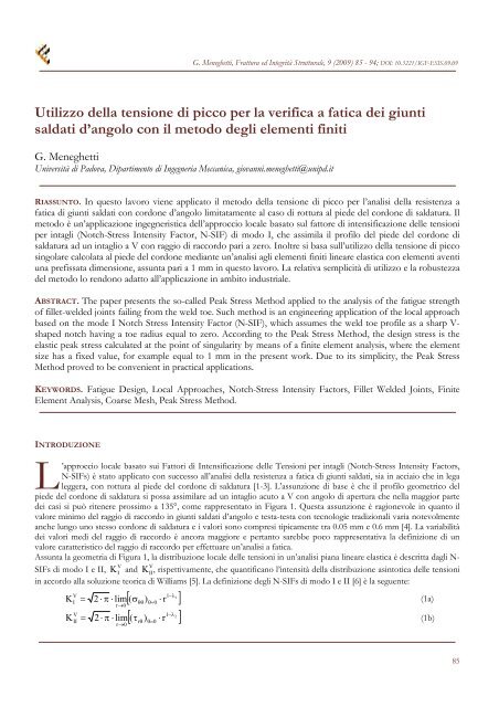
<strong>Utilizzo</strong> <strong>del<strong>la</strong></strong> <strong>tensione</strong> <strong>di</strong> <strong>picco</strong> <strong>per</strong> <strong>la</strong> <strong>verifica</strong> a <strong>fatica</strong> <strong>dei</strong> <strong>giunti</strong><br />
saldati d’angolo con il metodo degli elementi finiti<br />
G. Meneghetti<br />
Università <strong>di</strong> Padova, Dipartimento <strong>di</strong> Ingegneria Meccanica, giovanni.meneghetti@unipd.it<br />
RIASSUNTO. In questo <strong>la</strong>voro viene applicato il metodo <strong>del<strong>la</strong></strong> <strong>tensione</strong> <strong>di</strong> <strong>picco</strong> <strong>per</strong> l’analisi <strong>del<strong>la</strong></strong> resistenza a<br />
<strong>fatica</strong> <strong>di</strong> <strong>giunti</strong> saldati con cordone d’angolo limitatamente al caso <strong>di</strong> rottura al piede del cordone <strong>di</strong> saldatura. Il<br />
metodo è un’applicazione ingegneristica dell’approccio locale basato sul fattore <strong>di</strong> intensificazione delle tensioni<br />
<strong>per</strong> intagli (Notch-Stress Intensity Factor, N-SIF) <strong>di</strong> modo I, che assimi<strong>la</strong> il profilo del piede del cordone <strong>di</strong><br />
saldatura ad un intaglio a V con raggio <strong>di</strong> raccordo pari a zero. Inoltre si basa sull’utilizzo <strong>del<strong>la</strong></strong> <strong>tensione</strong> <strong>di</strong> <strong>picco</strong><br />
singo<strong>la</strong>re calco<strong>la</strong>ta al piede del cordone me<strong>di</strong>ante un’analisi agli elementi finiti lineare e<strong>la</strong>stica con elementi aventi<br />
una prefissata <strong>di</strong>mensione, assunta pari a 1 mm in questo <strong>la</strong>voro. La re<strong>la</strong>tiva semplicità <strong>di</strong> utilizzo e <strong>la</strong> robustezza<br />
del metodo lo rendono adatto all’applicazione in ambito industriale.<br />
ABSTRACT. The pa<strong>per</strong> presents the so-called Peak Stress Method applied to the analysis of the fatigue strength<br />
of fillet-welded joints failing from the weld toe. Such method is an engineering application of the local approach<br />
based on the mode I Notch Stress Intensity Factor (N-SIF), which assumes the weld toe profile as a sharp V-<br />
shaped notch having a toe ra<strong>di</strong>us equal to zero. Accor<strong>di</strong>ng to the Peak Stress Method, the design stress is the<br />
e<strong>la</strong>stic peak stress calcu<strong>la</strong>ted at the point of singu<strong>la</strong>rity by means of a finite element analysis, where the element<br />
size has a fixed value, for example equal to 1 mm in the present work. Due to its simplicity, the Peak Stress<br />
Method proved to be convenient in practical applications.<br />
KEYWORDS. Fatigue Design, Local Approaches, Notch-Stress Intensity Factors, Fillet Welded Joints, Finite<br />
Element Analysis, Coarse Mesh, Peak Stress Method.<br />
INTRODUZIONE<br />
L<br />
’approccio locale basato sui Fattori <strong>di</strong> Intensificazione delle Tensioni <strong>per</strong> intagli (Notch-Stress Intensity Factors,<br />
N-SIFs) è stato applicato con successo all’analisi <strong>del<strong>la</strong></strong> resistenza a <strong>fatica</strong> <strong>di</strong> <strong>giunti</strong> saldati, sia in acciaio che in lega<br />
leggera, con rottura al piede del cordone <strong>di</strong> saldatura [1-3]. L’assunzione <strong>di</strong> base è che il profilo geometrico del<br />
piede del cordone <strong>di</strong> saldatura si possa assimi<strong>la</strong>re ad un intaglio acuto a V con angolo <strong>di</strong> a<strong>per</strong>tura che nel<strong>la</strong> maggior parte<br />
<strong>dei</strong> casi si può ritenere prossimo a 135°, come rappresentato in Figura 1. Questa assunzione è ragionevole in quanto il<br />
valore minimo del raggio <strong>di</strong> raccordo in <strong>giunti</strong> saldati d’angolo e testa-testa con tecnologie tra<strong>di</strong>zionali varia notevolmente<br />
anche lungo uno stesso cordone <strong>di</strong> saldatura e i valori sono compresi tipicamente tra 0.05 mm e 0.6 mm [4]. La variabilità<br />
<strong>dei</strong> valori me<strong>di</strong> del raggio <strong>di</strong> raccordo è ancora maggiore e <strong>per</strong>tanto sarebbe poco rappresentativa <strong>la</strong> definizione <strong>di</strong> un<br />
valore caratteristico del raggio <strong>di</strong> raccordo <strong>per</strong> effettuare un’analisi a <strong>fatica</strong>.<br />
Assunta <strong>la</strong> geometria <strong>di</strong> Figura 1, <strong>la</strong> <strong>di</strong>stribuzione locale delle tensioni in un’analisi piana lineare e<strong>la</strong>stica è descritta dagli N-<br />
V<br />
V<br />
SIFs <strong>di</strong> modo I e II, K<br />
I<br />
and K<br />
II, rispettivamente, che quantificano l’intensità <strong>del<strong>la</strong></strong> <strong>di</strong>stribuzione asintotica delle tensioni<br />
in accordo al<strong>la</strong> soluzione teorica <strong>di</strong> Williams [5]. La definizione degli N-SIFs <strong>di</strong> modo I e II [6] è <strong>la</strong> seguente:<br />
1<br />
)<br />
0<br />
r <br />
1<br />
) r <br />
V<br />
1<br />
K 2 lim (<br />
(1a)<br />
I<br />
r0<br />
V<br />
2<br />
K 2<br />
lim (<br />
(1b)<br />
II<br />
r0<br />
r<br />
0<br />
85
G. Meneghetti, Frattura ed Integrità Strutturale, 9 (2009) 85 - 94; DOI: 10.3221/IGF-ESIS.09.09<br />
Figura 1: Modello geometrico <strong>di</strong> un giunto saldato d’angolo e sistema <strong>di</strong> riferimento po<strong>la</strong>re con origine al piede del cordone.<br />
Nelle precedenti definizioni, r e sono le coor<strong>di</strong>nate po<strong>la</strong>ri mostrate in Fig. 1, 1 , 2 sono gli autovalori <strong>di</strong> Williams <strong>per</strong><br />
modo I e II, rispettivamente. Quando l’angolo <strong>di</strong> a<strong>per</strong>tura è pari a 135°, l’esponente (1- 1) risulta 0.326 mentre (1- 2)<br />
risulta –0.302. Le componenti dello stato <strong>di</strong> <strong>tensione</strong> si possono infine esprimere nel<strong>la</strong> forma [1]:<br />
<br />
<br />
f1,<br />
(<br />
)<br />
<br />
f2,<br />
(<br />
)<br />
<br />
0.326<br />
V 0.302 V <br />
rr r KI<br />
f1,r<br />
( )<br />
r KII<br />
f2,r<br />
( )<br />
<br />
(2)<br />
<br />
<br />
<br />
r<br />
<br />
f1,r(<br />
)<br />
<br />
f2,r(<br />
)<br />
<br />
dove le funzioni f sono espressioni trigonometriche note. Le espressioni (2) mostrano che, essendo 2=135°, so<strong>la</strong>mente <strong>la</strong><br />
<strong>di</strong>stribuzione <strong>di</strong> modo I è singo<strong>la</strong>re.<br />
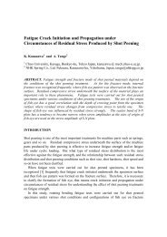
La Fig. 2 mostra come esempio il campo <strong>di</strong> <strong>tensione</strong> locale lungo <strong>la</strong> <strong>la</strong>miera principale <strong>di</strong> un giunto saldato d’angolo con<br />
doppio irrigi<strong>di</strong>mento. È evidente che solo il contributo <strong>di</strong> modo I allo stato <strong>di</strong> <strong>tensione</strong> locale è singo<strong>la</strong>re, mentre il<br />
contributo <strong>di</strong> modo II tende a zero. Nel<strong>la</strong> figura è anche riportato <strong>per</strong> confronto il risultato ottenuto con un’analisi piana<br />
lineare e<strong>la</strong>stica agli elementi finiti. Utilizzando i risultati dell’analisi agli elementi finiti ottenuti lungo <strong>la</strong> bisettrice<br />
V<br />
dell’intaglio e applicando <strong>la</strong> definizione (1a) è possibile calco<strong>la</strong>re K<br />
I<br />
, parametro da cui <strong>di</strong>pende <strong>la</strong> resistenza a <strong>fatica</strong>.<br />
Infatti esprimendo in sintesi l’approccio locale, è possibile affermare che due <strong>giunti</strong> saldati che in una prova <strong>di</strong> <strong>fatica</strong><br />
V<br />
s<strong>per</strong>imentano lo stesso range <strong>di</strong> variazione <strong>di</strong> K<br />
I<br />
avranno <strong>la</strong> stessa vita a <strong>fatica</strong>, qualunque sia <strong>la</strong> loro geometria e <strong>la</strong> loro<br />
<strong>di</strong>mensione assoluta.<br />
Tuttavia <strong>la</strong> Fig. 2 mostra che <strong>la</strong> densità <strong>del<strong>la</strong></strong> mesh necessaria <strong>per</strong> calco<strong>la</strong>re <strong>la</strong> <strong>di</strong>stribuzione asintotica del campo locale, e<br />
quin<strong>di</strong> il fattore <strong>di</strong> intensificazione <strong>di</strong> modo I, è elevata. Pertanto le fasi <strong>di</strong> preparazione <strong>del<strong>la</strong></strong> mesh, <strong>di</strong> calcolo e <strong>di</strong> analisi<br />
<strong>dei</strong> risultati risultano <strong>di</strong>spen<strong>di</strong>ose in termini <strong>di</strong> tempo. Si nota che in Fig. 2 <strong>la</strong> <strong>di</strong>mensione degli elementi più <strong>picco</strong>li<br />
utilizzati è una frazione <strong>di</strong> micron. L’analisi agli elementi finiti risulta inoltre ancora più complicata <strong>per</strong> <strong>giunti</strong> aventi<br />
geometria tri<strong>di</strong>mensionale come ad esempio i <strong>giunti</strong> con attacchi longitu<strong>di</strong>nali.<br />
10<br />
rr / n<br />
L/t = 1<br />
t = 12 mm<br />
h = 10 mm<br />
t<br />
L<br />
h<br />
r<br />
1<br />
Modo I<br />
Modo I+II<br />
FEM<br />
Modo II<br />
0.1<br />
0.001 0.01 0.1 1 10 100<br />
r (mm)<br />
Figura 2: confronto fra risultati analitici e numerici nel<strong>la</strong> valutazione dello stato tensionale lungo <strong>la</strong> su<strong>per</strong>ficie <strong>di</strong> un giunto saldato.<br />
86
G. Meneghetti, Frattura ed Integrità Strutturale, 9 (2009) 85 - 94; DOI: 10.3221/IGF-ESIS.09.09<br />
Il metodo <strong>del<strong>la</strong></strong> <strong>tensione</strong> <strong>di</strong> <strong>picco</strong> su<strong>per</strong>a questi problemi <strong>di</strong> applicazione dell’approccio N-SIF nell’analisi <strong>del<strong>la</strong></strong> resistenza a<br />
V<br />
<strong>fatica</strong> <strong>dei</strong> <strong>giunti</strong> saldati, sostituendo al parametro K<br />
I<br />
<strong>la</strong> <strong>tensione</strong> <strong>di</strong> <strong>picco</strong> singo<strong>la</strong>re calco<strong>la</strong>ta a piede cordone, che risulta<br />
più facile da calco<strong>la</strong>re con un’analisi agli elementi finiti. Pertanto dopo aver presentato le basi teoriche del metodo, ne<br />
verrà mostrata l’applicazione all’analisi <strong>del<strong>la</strong></strong> resistenza a <strong>fatica</strong> <strong>di</strong> <strong>giunti</strong> d’angolo aventi geometria semplice. Questa analisi<br />
consente <strong>di</strong> tarare due curve <strong>di</strong> resistenza a <strong>fatica</strong> in termini <strong>di</strong> <strong>tensione</strong> <strong>di</strong> <strong>picco</strong>, valide <strong>per</strong> <strong>giunti</strong> saldati d’angolo in<br />
acciaio e in lega leggera, rispettivamente, senza trattamenti post-saldatura. Successivamente queste curve <strong>di</strong> resistenza a<br />
<strong>fatica</strong> <strong>di</strong> progetto verranno utilizzate <strong>per</strong> stimare <strong>la</strong> resistenza a <strong>fatica</strong> <strong>di</strong> <strong>giunti</strong> aventi geometria più complessa.<br />
IL METODO DELLA TENSIONE DI PICCO<br />
Q<br />
uando si considera un componente contenente punti <strong>di</strong> singo<strong>la</strong>rità, ad esempio l’apice <strong>di</strong> una cricca o <strong>di</strong> un intaglio<br />
a<strong>per</strong>to a spigolo vivo, <strong>la</strong> <strong>tensione</strong> calco<strong>la</strong>ta all’apice con un’analisi lineare e<strong>la</strong>stica agli elementi finiti <strong>di</strong>pende dal<strong>la</strong><br />
fittezza <strong>del<strong>la</strong></strong> mesh, in modo che <strong>la</strong> <strong>tensione</strong> è tanto più elevata quanto minore è <strong>la</strong> <strong>di</strong>mensione degli elementi<br />
utilizzati. Pertanto <strong>la</strong> <strong>tensione</strong> singo<strong>la</strong>re calco<strong>la</strong>ta con gli elementi finiti non ha significato.<br />
Tuttavia Nisitani e Teranishi [7] hanno mostrato che <strong>la</strong> <strong>tensione</strong> singo<strong>la</strong>re peak calco<strong>la</strong>ta all’apice <strong>di</strong> una cricca con<br />
un’analisi lineare e<strong>la</strong>stica agli elementi finiti è in rapporto costante con il fattore <strong>di</strong> intensificazione delle tensioni K I<br />
(K I / peak = costante), purché sia mantenuta costante <strong>la</strong> <strong>di</strong>mensione e il tipo <strong>di</strong> elemento utilizzato.<br />
Recentemente, è stata data una giustificazione teorica al metodo <strong>del<strong>la</strong></strong> <strong>tensione</strong> <strong>di</strong> <strong>picco</strong> (PSM) [8] ed il suo utilizzo è stato<br />
esteso a casi <strong>di</strong>versi da quelli considerati in origine da Nisitani e Teranishi. In partico<strong>la</strong>re il PSM è stato esteso a casi <strong>di</strong><br />
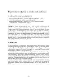
intagli a<strong>per</strong>ti a V a spigolo vivo ed è stato valutato l’effetto <strong>del<strong>la</strong></strong> <strong>di</strong>mensione degli elementi utilizzati <strong>per</strong> l’analisi. La Fig. 3<br />
mostra <strong>di</strong>verse geometrie contenenti punti <strong>di</strong> singo<strong>la</strong>rità dovuti a cricche o intagli a spigolo vivo. Per ognuna <strong>di</strong> queste<br />
geometrie è stata fatta variare <strong>la</strong> profon<strong>di</strong>tà dell’intaglio o <strong>del<strong>la</strong></strong> cricca a parità <strong>di</strong> <strong>di</strong>mensione <strong>di</strong> elemento oppure <strong>la</strong><br />
<strong>di</strong>mensione dell’elemento a parità <strong>di</strong> <strong>di</strong>mensione <strong>di</strong> intaglio o cricca. Le analisi agli elementi finiti lineari e<strong>la</strong>stiche sono<br />
state fatte con il co<strong>di</strong>ce Ansys utilizzando gli elementi quadrango<strong>la</strong>ri a quattro no<strong>di</strong> PLANE 42. La mesh è stata generata<br />
automaticamente dal software una volta imposta <strong>la</strong> <strong>di</strong>mensione dell’elemento d con il comando ‘global element size’.<br />
Nessun altro controllo sul<strong>la</strong> forma e <strong>di</strong>mensione degli elementi è stato utilizzato.<br />
Figura 3: geometrie contenenti punti <strong>di</strong> singo<strong>la</strong>rità tensionale utilizzate <strong>per</strong> validare il<br />
metodo <strong>del<strong>la</strong></strong> <strong>tensione</strong> <strong>di</strong> <strong>picco</strong> (<strong>di</strong>mensioni in mm) [8].<br />
87
G. Meneghetti, Frattura ed Integrità Strutturale, 9 (2009) 85 - 94; DOI: 10.3221/IGF-ESIS.09.09<br />
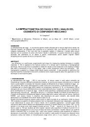
I risultati sono riportati nel<strong>la</strong> Fig. 4, che mostra, al variare del rapporto tra <strong>la</strong> <strong>di</strong>mensione <strong>di</strong> riferimento a del componente<br />
e <strong>la</strong> <strong>di</strong>mensione d dell’elemento, il parametro a<strong>di</strong>mensionale K :<br />
K<br />
*<br />
FE<br />
peak<br />
*<br />
FE<br />
V<br />
K<br />
I<br />
11<br />
d<br />
(3)<br />
calco<strong>la</strong>to <strong>per</strong> ogni geometria presa in considerazione. La Fig. 4 mostra che non appena a/d è maggiore o uguale a 3, il<br />
*<br />
parametro K<br />
FE<br />
è pressoché costante e pari a 1.38, con risultati numerici raccolti in una ristretta banda definita dal +-3%<br />
*<br />
rispetto a tale valore. In [8] è fornita anche un’espressione analitica <strong>per</strong> calco<strong>la</strong>re il parametro K<br />
FE<br />
. Scelta quin<strong>di</strong> una certa<br />
<strong>di</strong>mensione <strong>di</strong> elemento d da utilizzare nelle analisi agli elementi finiti, <strong>la</strong> Fig. 4 e l’Eq. (3), dove K * FE<br />
1. 38 , mostrano che<br />
il rapporto<br />
V<br />
K I<br />
<br />
peak<br />
è costante e quin<strong>di</strong> <strong>la</strong> <strong>tensione</strong> <strong>di</strong> <strong>picco</strong> peak può sostituire l’N-SIF<br />
V<br />
K<br />
I<br />
nelle analisi <strong>di</strong> resistenza a<br />
<strong>fatica</strong> con notevole riduzione <strong>dei</strong> tempi e semplificazione delle procedure <strong>di</strong> calcolo. È necessario tener presente che il<br />
metodo <strong>del<strong>la</strong></strong> <strong>tensione</strong> <strong>di</strong> <strong>picco</strong> così come presentato è valido sotto le seguenti con<strong>di</strong>zioni:<br />
- Elementi lineari quadri<strong>la</strong>teri a quattro no<strong>di</strong> (PLANE 42, <strong>del<strong>la</strong></strong> libreria del co<strong>di</strong>ce ANSYS 8.0);<br />
- Pattern <strong>di</strong> elementi come quello riportato nel<strong>la</strong> successiva Fig. 5;<br />
- Intagli a V con angolo <strong>di</strong> a<strong>per</strong>tura compreso tra 0° e 135°.<br />
K * FE<br />
2.2<br />
2<br />
1.8<br />
1.6<br />
Fig. 6a, a=variabile, d=1 mm<br />
Fig. 6b, a=variabile, d=1 mm<br />
Fig. 6b, a=10 mm, d=variabile<br />
Fig. 6c, 2=135°, a=10 mm, d=variabile<br />
Fig. 6c, 2=90°, a=5 mm, d=variabile<br />
Fig. 6c, 2=90°, a=10 mm, d=variabile<br />
Fig. 6c, 2=90°, a=15 mm, d=variabile<br />
Fig. 6d, a/b/t=13/10/8, d=variabile<br />
Fig. 6d, a/b/t=100/50/16, d=variabile<br />
Valore me<strong>di</strong>o<br />
1.4<br />
1.2<br />
Limiti <strong>di</strong> vali<strong>di</strong>tà del PSM<br />
3%<br />
1<br />
1 3<br />
10 a/d 100<br />
*<br />
Figura 4: parametro a<strong>di</strong>mensionale K FE ottenuto da 61 analisi agli elementi finiti delle<br />
geometrie riportate in Fig. 5. La linea continua rappresenta il valor me<strong>di</strong>o pari a 1.38 [8].<br />
DEFINIZIONE DI CURVE DI RESISTENZA A FATICA DI PROGETTO PER GIUNTI SALDATI D’ANGOLO IN<br />
ACCIAIO E IN LEGA LEGGERA<br />
L<br />
a possibilità <strong>di</strong> definire bande <strong>di</strong> resistenza a <strong>fatica</strong> unificate, al variare <strong>del<strong>la</strong></strong> geometria e delle <strong>di</strong>mensioni assolute,<br />
V V<br />
<strong>per</strong> <strong>giunti</strong> in acciaio e in lega leggera saldati d’angolo in termini <strong>di</strong> range <strong>di</strong> variazione <strong>di</strong> K<br />
I<br />
, K I<br />
, è già stata<br />
<strong>verifica</strong>ta in passato [1, 3]. Essendo valida l’Eq. (3) con K * FE<br />
1. 38 e una volta scelta <strong>la</strong> <strong>di</strong>mensione <strong>di</strong> elemento<br />
utilizzata nell’analisi agli elementi finiti, è quin<strong>di</strong> possibile definire delle curve <strong>di</strong> progetto <strong>di</strong> resistenza a <strong>fatica</strong> in termini <strong>di</strong><br />
range <strong>del<strong>la</strong></strong> <strong>tensione</strong> <strong>di</strong> <strong>picco</strong> peak. A tale scopo sono stati utilizzati i dati <strong>di</strong> Maddox [9], Gurney [10, 11], Kihl and<br />
Sarkani [12, 13] pubblicati negli articoli originali in termini <strong>di</strong> <strong>tensione</strong> nominale. I dettagli sulle geometrie, i materiali e le<br />
con<strong>di</strong>zioni <strong>di</strong> carico sono riportati in [8]. In sintesi, i dati si riferiscono a <strong>giunti</strong> in acciaio da costruzione (con <strong>tensione</strong> <strong>di</strong><br />
snervamento variabile tra 360 e 670 MPa) e in leghe leggere <strong>del<strong>la</strong></strong> serie 5000 e 6000 (con <strong>tensione</strong> <strong>di</strong> snervamento variabile<br />
fra 250 e 304 MPa) sollecitati a trazione o flessione con rapporto nominale <strong>di</strong> ciclo R (definito come rapporto fra <strong>la</strong><br />
<strong>tensione</strong> nominale minima e quel<strong>la</strong> massima applicata) prossimo a zero. Tutti i <strong>giunti</strong> hanno semplice configurazione a T o<br />
a croce con saldature d’angolo e sono stati sottoposti a prova senza alcun trattamento post-saldatura. I <strong>giunti</strong> in acciaio<br />
88
G. Meneghetti, Frattura ed Integrità Strutturale, 9 (2009) 85 - 94; DOI: 10.3221/IGF-ESIS.09.09<br />
hanno spessore del piatto principale variabile fra 6 e 100 mm con rapporto tra gli spessori saldati compreso fra 0.03 e 8.8,<br />
mentre quelli in lega leggera fra 3 e 24 mm con rapporto tra gli spessori saldati variabile fra 0.25 e 1.<br />
Nodo in cui calco<strong>la</strong>re <strong>la</strong> <strong>tensione</strong><br />
massima principale ( peak )<br />
d = 1 mm<br />
Y<br />
Z<br />
X<br />
Figura 5: mesh free utilizzata <strong>per</strong> le analisi agli elementi finiti <strong>di</strong> <strong>giunti</strong> saldati d’angolo con elementi <strong>di</strong> <strong>di</strong>mensione pari a 1 mm.<br />
<br />
R 0<br />
peak [MPa]<br />
<br />
<br />
Pendenza<br />
k = 3.00<br />
<br />
T =<br />
<br />
A,2.3%<br />
A,97.7%<br />
=1.90<br />
D, 50% = 149 MPa<br />
<br />
4 5 6 7<br />
N. cicli a rottura<br />
205<br />
D, 50%<br />
108<br />
Figura 6: resistenza a <strong>fatica</strong> <strong>di</strong> <strong>giunti</strong> saldati d’angolo in acciaio da costruzione in termini <strong>di</strong> <strong>tensione</strong> <strong>di</strong> <strong>picco</strong> lineare e<strong>la</strong>stica calco<strong>la</strong>ta<br />
con <strong>la</strong> mesh riportata in Fig. 5. Banda <strong>di</strong> <strong>di</strong>s<strong>per</strong>sione re<strong>la</strong>tiva al valor me<strong>di</strong>o due deviazioni standard [8].<br />
peak [MPa]<br />
<br />
<br />
<br />
<br />
<br />
<br />
Pendenza<br />
k = 3.80<br />
<br />
T =<br />
<br />
4 5 6 7<br />
94<br />
D, 50%<br />
52<br />
N. cicli a rottura<br />
Figura 7: resistenza a <strong>fatica</strong> <strong>di</strong> <strong>giunti</strong> saldati d’angolo in lega leggera in termini <strong>di</strong> <strong>tensione</strong> <strong>di</strong> <strong>picco</strong> lineare e<strong>la</strong>stica calco<strong>la</strong>ta usando<br />
elementi <strong>di</strong> 1 mm <strong>di</strong> <strong>di</strong>mensione come riportato in Fig. 5. Banda <strong>di</strong> <strong>di</strong>s<strong>per</strong>sione re<strong>la</strong>tiva al valor me<strong>di</strong>o due deviazioni standard [8].<br />
Le analisi numeriche sono state fatte con il software Ansys usando mesh <strong>di</strong> tipo free con elementi <strong>di</strong> <strong>di</strong>mensione <strong>di</strong> 1 mm<br />
come riportato in Fig. 5 e imponendo una <strong>tensione</strong> nominale pari a 1 MPa. Calco<strong>la</strong>ndo <strong>la</strong> <strong>tensione</strong> massima principale<br />
( peak) nel punto <strong>di</strong> singo<strong>la</strong>rità è stato possibile esprimere i risultati originali in termini <strong>di</strong> range <strong>di</strong> <strong>tensione</strong> <strong>di</strong> <strong>picco</strong> anziché<br />
R 0<br />
A,2.3%<br />
A,97.7%<br />
=1.81<br />
89
G. Meneghetti, Frattura ed Integrità Strutturale, 9 (2009) 85 - 94; DOI: 10.3221/IGF-ESIS.09.09<br />
range <strong>di</strong> <strong>tensione</strong> nominale. I risultati sono riportati in Fig. 6 e 7 <strong>per</strong> i <strong>giunti</strong> in acciaio e in lega leggera, rispettivamente. Le<br />
bande <strong>di</strong> <strong>di</strong>s<strong>per</strong>sione riportate si riferiscono a probabilità <strong>di</strong> sopravvivenza del 97.7% e il parametro T che ne quantifica<br />
l’ampiezza risulta confrontabile con i valori trovati in termini <strong>di</strong> N-SIF [3]. Considerando ulteriormente i <strong>giunti</strong> in acciaio e<br />
calco<strong>la</strong>ndo il parametro T <strong>per</strong> probabilità <strong>di</strong> sopravvivenza del 10% e 90% si trova 1.51 in ottimo accordo con il valore <strong>di</strong><br />
1.50 re<strong>la</strong>tivo al<strong>la</strong> banda unificata proposta da Haibach [14]. Pertanto è possibile concludere che le bande riportate nelle<br />
Fig. 6 e 7 si possono ritenere bande unificate <strong>per</strong> <strong>la</strong> progettazione a <strong>fatica</strong> <strong>di</strong> <strong>giunti</strong> saldati d’angolo in acciaio da<br />
costruzione e lega leggera, rispettivamente, senza trattamenti post-saldatura e <strong>per</strong> rotture innescate a piede cordone.<br />
APPLICAZIONE DEL METODO DELLA TENSIONE DI PICCO A GIUNTI COMPLESSI<br />
L<br />
e curve <strong>di</strong> resistenza a <strong>fatica</strong> riportate nelle Fig. 6 e 7 sono state utilizzate <strong>per</strong> stimare <strong>la</strong> resistenza a <strong>fatica</strong> <strong>di</strong> <strong>giunti</strong><br />
saldati d’angolo aventi geometria complessa presenti in letteratura.<br />
Le Tab. 1 e 2 riportano le geometrie <strong>di</strong> giunto analizzate <strong>per</strong> acciai e leghe leggere, rispettivamente, mentre <strong>per</strong> i<br />
dettagli riguardo ai materiali e ai riferimenti ai <strong>la</strong>vori originali si rimanda a [15]. Le geometrie <strong>dei</strong> <strong>giunti</strong> sono del tipo con<br />
irrigi<strong>di</strong>mento longitu<strong>di</strong>nale, single-<strong>la</strong>p o tubo<strong>la</strong>re come riportato nelle Tab. 1 e 2. Per quanto riguarda i <strong>giunti</strong> in acciaio, i<br />
materiali impiegati sono acciai da costruzione con <strong>tensione</strong> <strong>di</strong> snervamento compresa fra 309 e 780 MPa, gli spessori<br />
variabili fra 3 e 12.5 mm, mentre il rapporto <strong>di</strong> ciclo è compreso fra 0 e 0.7. Per quanto riguarda i <strong>giunti</strong> in lega leggera, i<br />
materiali impiegati sono leghe <strong>del<strong>la</strong></strong> serie 5000 e 6000 aventi <strong>tensione</strong> <strong>di</strong> snervamento compresa fra 245 e 290 MPa, gli<br />
spessori sono variabili fra 3 e 12 mm, mentre il rapporto <strong>di</strong> ciclo è compreso è prossimo a zero.<br />
Le analisi agli elementi finiti <strong>dei</strong> <strong>giunti</strong> bi<strong>di</strong>mensionali, come ad esempio i <strong>giunti</strong> single-<strong>la</strong>p, sono state condotte utilizzando<br />
<strong>la</strong> mesh riportata in Figura 5, mentre <strong>per</strong> calco<strong>la</strong>re <strong>la</strong> <strong>tensione</strong> <strong>di</strong> <strong>picco</strong> nel caso <strong>di</strong> <strong>giunti</strong> tubo<strong>la</strong>ri è stata utilizzata <strong>la</strong><br />
procedura a due step dettagliata in [15, 16] e riassunta dal<strong>la</strong> Fig. 8.<br />
Nel primo step <strong>di</strong> analisi è stato definito un modello ad elementi shell (modello principale). Nel secondo step <strong>di</strong> analisi si è<br />
immaginato <strong>di</strong> fare una sezione longitu<strong>di</strong>nale del giunto reale in corrispondenza del punto <strong>di</strong> innesco <strong>del<strong>la</strong></strong> rottura a <strong>fatica</strong><br />
del giunto con un piano che nel caso <strong>di</strong> Fig. 8 stacca sul<strong>la</strong> su<strong>per</strong>ficie del modello principale le due linee spesse. Si ottiene<br />
così il sottomodello riportato in Fig. 8 che riproduce lo spessore degli elementi saldati e il profilo a V a spigolo vivo del<br />
piede del cordone. I risultati dell’analisi sul modello principale, a cui sono applicate le con<strong>di</strong>zioni al contorno, sono<br />
trasferiti al sottomodello imponendo una con<strong>di</strong>zione <strong>di</strong> congruenza, ovvero gli spostamenti calco<strong>la</strong>ti lungo le linee spesse<br />
del modello principale vengono imposti alle corrispondenti linee spesse del sottomodello. Questa o<strong>per</strong>azione è effettuata<br />
automaticamente in ambiente Ansys utilizzando il comando ‘shell-to-solid’ submodeling.<br />
Le Fig. 9 e 10 riportano il confronto fra i risultati s<strong>per</strong>imentali e le curve <strong>di</strong> progetto riportate nelle Fig. 6 e 7,<br />
rispettivamente, <strong>per</strong> i <strong>giunti</strong> in acciaio e in lega leggera. Dal confronto si nota <strong>la</strong> vali<strong>di</strong>tà delle curve <strong>di</strong> progetto, fatta<br />
eccezione <strong>per</strong> i <strong>giunti</strong> <strong>di</strong> più <strong>picco</strong>lo spessore, che meritano ulteriori approfon<strong>di</strong>menti [15]. Nelle strutture reali i <strong>per</strong>corsi<br />
<strong>di</strong> propagazione possono essere multipli oppure partico<strong>la</strong>rmente lunghi, in modo tale da rendere significativa <strong>la</strong> quota<br />
parte <strong>di</strong> vita a <strong>fatica</strong> spesa <strong>per</strong> <strong>la</strong> propagazione <strong>di</strong> cricche al <strong>di</strong> fuori del <strong>picco</strong>lo volume <strong>di</strong> materiale in cui lo stato <strong>di</strong><br />
<strong>tensione</strong> è control<strong>la</strong>to dagli N-SIFs. In questi casi le curve <strong>di</strong> progetto riportate nelle Figure 6 e 7 vanno utilizzate <strong>per</strong><br />
stimare <strong>la</strong> vita <strong>fatica</strong> a innesco, mentre <strong>per</strong> <strong>la</strong> fase <strong>di</strong> propagazione è valido il c<strong>la</strong>ssico approccio basato sul<strong>la</strong> Meccanica<br />
<strong>del<strong>la</strong></strong> Frattura Lineare E<strong>la</strong>stica.<br />
Si ritiene infine che utilizzando il metodo <strong>del<strong>la</strong></strong> <strong>tensione</strong> <strong>di</strong> <strong>picco</strong> unitamente al<strong>la</strong> procedura <strong>di</strong> calcolo descritta, l’approccio<br />
N-SIF <strong>per</strong> <strong>la</strong> progettazione a <strong>fatica</strong> <strong>dei</strong> <strong>giunti</strong> saldati possa essere implementato in un contesto industriale.<br />
CONCLUSIONI<br />
I<br />
l metodo <strong>del<strong>la</strong></strong> <strong>tensione</strong> <strong>di</strong> <strong>picco</strong> (PSM) è stato applicato all’analisi <strong>del<strong>la</strong></strong> resistenza a <strong>fatica</strong> <strong>di</strong> <strong>giunti</strong> saldati d’angolo in<br />
acciaio e in lega leggera senza trattamenti post-saldatura con rottura al piede del cordone <strong>di</strong> saldatura. Il metodo<br />
proposto è un’applicazione ingegneristica dell’approccio locale basato sugli N-SIF, che assimi<strong>la</strong> il profilo geometrico<br />
del piede del cordone <strong>di</strong> saldatura ad un intaglio a V a spigolo vivo con angolo <strong>di</strong> a<strong>per</strong>tura tipicamente pari a 135°. Il<br />
metodo <strong>del<strong>la</strong></strong> <strong>tensione</strong> <strong>di</strong> <strong>picco</strong> utilizza come <strong>tensione</strong> <strong>di</strong> progetto <strong>la</strong> <strong>tensione</strong> <strong>di</strong> <strong>picco</strong> singo<strong>la</strong>re calco<strong>la</strong>ta al piede cordone<br />
con un’analisi agli elementi in cui <strong>la</strong> <strong>di</strong>mensione degli elementi sia prefissata, pari a 1 mm in questo <strong>la</strong>voro. La tecnica <strong>di</strong><br />
analisi è presentata nelle Figure 5 e 8 <strong>per</strong> <strong>giunti</strong> aventi geometria riconducibile a modelli bi<strong>di</strong>mensionali e tri<strong>di</strong>mensionali,<br />
rispettivamente. Le curve <strong>di</strong> resistenza a <strong>fatica</strong> da utilizzare <strong>per</strong> le verifiche sono riportate nelle Figure 6 e 7,<br />
rispettivamente, <strong>per</strong> <strong>giunti</strong> in acciaio e in lega leggera.<br />
90
G. Meneghetti, Frattura ed Integrità Strutturale, 9 (2009) 85 - 94; DOI: 10.3221/IGF-ESIS.09.09<br />
Geometria Tipo <strong>di</strong> carico Geometria Tipo <strong>di</strong> carico<br />
Tabel<strong>la</strong> 1: Geometria e con<strong>di</strong>zioni <strong>di</strong> carico <strong>per</strong> i <strong>giunti</strong> saldati d’angolo in acciaio considerati<br />
( n: range <strong>del<strong>la</strong></strong> <strong>tensione</strong> nominale considerata negli articoli originali; <strong>di</strong>mensioni in mm) [15].<br />
91
G. Meneghetti, Frattura ed Integrità Strutturale, 9 (2009) 85 - 94; DOI: 10.3221/IGF-ESIS.09.09<br />
Geometria<br />
Tipo <strong>di</strong> carico<br />
Tabel<strong>la</strong> 2: Geometria e con<strong>di</strong>zioni <strong>di</strong> carico <strong>per</strong> i <strong>giunti</strong> saldati d’angolo in lega leggera considerati<br />
( n : range <strong>del<strong>la</strong></strong> <strong>tensione</strong> nominale considerata negli articoli originali; <strong>di</strong>mensioni in mm) [15].<br />
92
G. Meneghetti, Frattura ed Integrità Strutturale, 9 (2009) 85 - 94; DOI: 10.3221/IGF-ESIS.09.09<br />
PRIMO STEP: analisi del ‘modello principale ’.<br />
Gli elementi shell vengono generati sul<strong>la</strong> su<strong>per</strong>ficie me<strong>di</strong>a<br />
Punto <strong>di</strong> innesco cricca<br />
virtuale<br />
Punto <strong>di</strong> innesco cricca<br />
( piede cordone )<br />
Gli spostamenti calco<strong>la</strong>ti<br />
lungo <strong>la</strong> linea evidenziata nel<br />
‘modello principale ’ sono<br />
trasferiti nelle corrispondenti<br />
posizioni del ‘ sottomodello ’.<br />
SECONDO STEP: analisi del ‘sottomodello’ .<br />
Mesh standard con elementi da 1 mm sul<strong>la</strong> sezione longitu<strong>di</strong>nale del giunto<br />
peak<br />
(nel punto <strong>di</strong> innesco)<br />
Punto <strong>di</strong> innesco cricca<br />
virtuale<br />
Figura 8: Tecnica <strong>di</strong> analisi agli elementi finiti <strong>di</strong> <strong>giunti</strong> tri<strong>di</strong>mensionali <strong>per</strong> calco<strong>la</strong>re <strong>la</strong> <strong>tensione</strong> <strong>di</strong> <strong>picco</strong> ( peak ) a piede cordone [15].<br />
5000<br />
1000<br />
peak [MPa]<br />
Giunti a croce n-l-c (3 mm < t < 10 mm)<br />
T nlc (t=5 and 6 mm)<br />
Giunti a croce lc (t= 3 and 6 mm)<br />
Lap joint (t= 3.2 mm)<br />
Attacchi longitu<strong>di</strong>nali (6 mm < t < 12 mm)<br />
Tubo-su-f<strong>la</strong>ngia (5 mm < t < 8 mm)<br />
Giunti tubo<strong>la</strong>ri a croce (t=12.5 mm)<br />
Simboli pieni: prove run-out<br />
Banda <strong>di</strong> <strong>di</strong>s<strong>per</strong>sione proposta (cfr Fig. 6)<br />
100<br />
1.E+04 1.E+05 1.E+06 1.E+07<br />
N. cicli a rottura<br />
Figura 9: Confronto fra <strong>la</strong> banda <strong>di</strong> <strong>di</strong>s<strong>per</strong>sione proposta in Fig. 6 e i risultati s<strong>per</strong>imentali in termini <strong>di</strong> range <strong>di</strong> <strong>tensione</strong> <strong>di</strong> <strong>picco</strong> <strong>per</strong><br />
<strong>giunti</strong> saldati d’angolo in acciaio (n-l-c: cordoni non portanti; lc: cordoni portanti) [15].<br />
93
G. Meneghetti, Frattura ed Integrità Strutturale, 9 (2009) 85 - 94; DOI: 10.3221/IGF-ESIS.09.09<br />
1000<br />
peak [MPa]<br />
100<br />
Giunti a croce nlc (t=8 mm)<br />
T nlc (t=3 mm and 8 mm)<br />
Lap joint (3 mm < t < 8 mm)<br />
Attacchi longitu<strong>di</strong>nali (t= 8 mm and 11 mm)<br />
RHS-to-RHS (t= 3 mm)<br />
Simboli pieni : prove run-out<br />
Banda <strong>di</strong> <strong>di</strong>s<strong>per</strong>sione proposta (cfr Fig. 7)<br />
20<br />
1.E+04 1.E+05 1.E+06<br />
N. cicli a rottura<br />
1.E+07<br />
Figura 10: Confronto fra <strong>la</strong> banda <strong>di</strong> <strong>di</strong>s<strong>per</strong>sione proposta in Fig. 6 e i risultati s<strong>per</strong>imentali in termini <strong>di</strong><br />
range <strong>di</strong> <strong>tensione</strong> <strong>di</strong> <strong>picco</strong> <strong>per</strong> <strong>giunti</strong> saldati d’angolo in lega leggera (n-l-c: cordoni non portanti;<br />
lc: cordoni portanti; RHS-to-RHS: giunto realizzato con elementi tubo<strong>la</strong>ri a sezione rettango<strong>la</strong>re) [15].<br />
BIBLIOGRAFIA<br />
[1] P. Lazzarin, R. Tovo, Fatigue Fract. Engng. Mater. Struct., 21 (1998)1089.<br />
[2] B. Atzori, G. Meneghetti, Int. J. Fatigue, 23(8) (2001) 713.<br />
[3] P. Lazzarin, P. Livieri, Int. J. Fatigue, 23 (2001) 225.<br />
[4] A. Seto, Y. Yoshida, A. Galtier, Fatigue Fract. Engng. Mater. Struct., 27 (2004) 1147.<br />
[5] M. L. Williams, J. Appl. Mech., 19 (1952) 526.<br />
[6] R. Gross, A. Mendelson, Int. J. Fract. Mech., 8 (1972) 267.<br />
[7] H. Nisitani, T. Teranishi, Engng. Fract. Mech., 71 (2004) 579.<br />
[8] G. Meneghetti, P. Lazzarin, Fatigue Fract. Engng. Mater. Struct., 30 (2007) 95.<br />
[9] S. J. Maddox, The effect of p<strong>la</strong>te thickness on the fatigue strength of fillet welded joints, Abington Publishing,<br />
Abington, Cambridge (1987).<br />
[10] T. R. Gurney, The fatigue strength of transverse fillet welded joints, Abington Publishing, Abington, Cambridge<br />
(1991).<br />
[11] T. R. Gurney, Fatigue of thin walled joints under complex loa<strong>di</strong>ng, Abington Publishing, Abington, Cambridge<br />
(1997).<br />
[12] D. P. Kihl, S. Sarkani, Int. J. Fatigue, 19 (1997) S311.<br />
[13] D. P. Kihl, S. Sarkani, Probab. Eng. Mech. , 14 (1999) 97.<br />
[14] E. Haibach Service fatigue-strength – methods and data for structural analysis, Dusseldorf, VDI (1989).<br />
[15] G. Meneghetti, Fatigue Fract. Engng. Mater. Struct., 31 (5) (2008) 346.<br />
[16] G. Meneghetti, F. Righetto, Atti del XXXV Convegno Nazionale AIAS, Ancona (2006).<br />
94