Estudo da qualidade do ar numa estação de Braga (Circular Sul) e ...
Estudo da qualidade do ar numa estação de Braga (Circular Sul) e ...
Estudo da qualidade do ar numa estação de Braga (Circular Sul) e ...

You also want an ePaper? Increase the reach of your titles
YUMPU automatically turns print PDFs into web optimized ePapers that Google loves.
Trabalho 2<br />
<strong>Estu<strong>do</strong></strong> <strong>da</strong> quali<strong>da</strong><strong>de</strong> <strong>do</strong> <strong>ar</strong> <strong>numa</strong> <strong>estação</strong> <strong>de</strong> <strong>Braga</strong> (Circul<strong>ar</strong> <strong>Sul</strong>) e em seis estações <strong>de</strong><br />
Lisboa<br />
Objectivos<br />
O primeiro objectivo a ser alcança<strong>do</strong> neste trabalho é proce<strong>de</strong>r a uma averiguação acerca <strong>da</strong><br />
existência ou não <strong>de</strong> uma relação entre o poluente p<strong>ar</strong>tículas inaláveis (PM10) e outros<br />
poluentes (NO, NO2 e CO) na <strong>estação</strong> <strong>de</strong> monitorização <strong>de</strong> quali<strong>da</strong><strong>de</strong> <strong>do</strong> <strong>ar</strong>, localiza<strong>da</strong> na<br />
Circul<strong>ar</strong> <strong>Sul</strong> - <strong>Braga</strong>.<br />
O segun<strong>do</strong> objectivo passa pela i<strong>de</strong>ntificação <strong>de</strong> comportamentos semelhantes,<br />
conjuntamente entre os poluentes referi<strong>do</strong>s anteriormente nas estações <strong>da</strong> Aveni<strong>da</strong> <strong>da</strong><br />
Liber<strong>da</strong><strong>de</strong>, <strong>de</strong> Olivais, Restelo e <strong>de</strong> Entrecampos, pertencentes ao concelho <strong>de</strong> Lisboa e<br />
ain<strong>da</strong> na <strong>estação</strong> <strong>da</strong> Reboleira /Ama<strong>do</strong>ra e Loures / Loures, através <strong>de</strong> uma análise em<br />
componentes principais.<br />
Introdução<br />
Enten<strong>de</strong>-se por quali<strong>da</strong><strong>de</strong> <strong>do</strong> <strong>ar</strong> como sen<strong>do</strong> o grau <strong>de</strong> poluição <strong>do</strong> <strong>ar</strong> que respiramos. Esta é<br />
causa<strong>da</strong> por uma mistura <strong>de</strong> substâncias químicas que são lança<strong>da</strong>s na atmosfera, ou então<br />
resultantes <strong>de</strong> reacções químicas que adulteram o esta<strong>do</strong> natural <strong>de</strong>sta. Estas substâncias<br />
poluentes po<strong>de</strong>m conduzir a um maior ou menor impacte ao nível <strong>da</strong> quali<strong>da</strong><strong>de</strong> <strong>do</strong> <strong>ar</strong>,<br />
consoante a sua composição química, concentração na massa <strong>de</strong> <strong>ar</strong> em causa e condições<br />
meteorológicas.<br />
As duas principais fontes emissoras <strong>de</strong> poluentes atmosféricos po<strong>de</strong>m ser <strong>de</strong> origem natural<br />
ou <strong>de</strong> origem antrópica. O primeiro tipo <strong>de</strong> poluição provém <strong>de</strong> fenómenos que ocorrem na<br />
natureza, tais como emissões provenientes <strong>de</strong> erupções vulcânicas ou fogos florestais <strong>de</strong><br />
origem natural, sen<strong>do</strong> que a poluição resultante <strong>de</strong> activi<strong>da</strong><strong>de</strong>s humanas (poluição<br />
antrópica), respeita à introdução <strong>de</strong> poluentes na atmosfera por activi<strong>da</strong><strong>de</strong>s industriais ou<br />
pelo tráfego automóvel. A poluição causa<strong>da</strong> pelo tráfego automóvel ten<strong>de</strong> a caus<strong>ar</strong> um<br />
maior impacto no ambiente circun<strong>da</strong>nte e ao nível <strong>do</strong> solo, que a poluição proveniente <strong>de</strong><br />
chaminés altas, sen<strong>do</strong> o tráfego automóvel causa<strong>do</strong>r <strong>de</strong> problemas <strong>de</strong> poluição no solo a<br />
uma maior distância <strong>da</strong> sua fonte.<br />
Com vista a alcanç<strong>ar</strong>mos os objectivos <strong>de</strong>ste trabalho, retirámos os <strong>da</strong><strong>do</strong>s relativos aos<br />
poluentes atmosféricos como as p<strong>ar</strong>tículas inaláveis (PM10), NO, NO2 e CO, referentes a
ca<strong>da</strong> <strong>estação</strong> <strong>do</strong> site <strong>da</strong> oficial <strong>da</strong> quali<strong>da</strong><strong>de</strong> <strong>do</strong> <strong>ar</strong>, www.qual<strong>ar</strong>.org, sen<strong>do</strong> estes <strong>da</strong><strong>do</strong>s<br />
posteriormente trabalha<strong>do</strong>s com o auxílio <strong>de</strong> <strong>do</strong>is softw<strong>ar</strong>es <strong>de</strong> nome Excel e SPSS.<br />
Resulta<strong>do</strong>s<br />
1. Estação <strong>de</strong> <strong>Braga</strong> (Circul<strong>ar</strong> <strong>Sul</strong>)<br />
Tabela 1 – Correlação entre as diferentes v<strong>ar</strong>iáveis.<br />
NO2<br />
PM10<br />
NO<br />
CO<br />
Pe<strong>ar</strong>son Correlation<br />
Sig. (2-tailed)<br />
N<br />
Pe<strong>ar</strong>son Correlation<br />
Sig. (2-tailed)<br />
N<br />
Pe<strong>ar</strong>son Correlation<br />
Sig. (2-tailed)<br />
N<br />
Pe<strong>ar</strong>son Correlation<br />
Sig. (2-tailed)<br />
N<br />
Correlations<br />
**. Correlation is significant at the 0.01 level (2-tailed).<br />
NO2 PM10 NO CO<br />
1 ,715** ,889** ,682**<br />
,000 ,000 ,000<br />
34 32 34 34<br />
,715** 1 ,671** ,548**<br />
,000 ,000 ,001<br />
32 32 32 32<br />
,889** ,671** 1 ,898**<br />
,000 ,000 ,000<br />
34 32 34 34<br />
,682** ,548** ,898** 1<br />
,000 ,001 ,000<br />
34 32 34 34<br />
Na tabela <strong>de</strong> correlação <strong>da</strong>s quatro v<strong>ar</strong>iáveis (CO, NO, PM10 e NO2) verifica-se que há<br />
uma maior correlação entre o CO e o NO uma vez que o coeficiente <strong>de</strong> Pe<strong>ar</strong>son (R) é o<br />
mais eleva<strong>do</strong> (com um valor <strong>de</strong> 0,898). Isto significa que o CO e o NO comportam-se <strong>de</strong><br />
forma semelhante.
Tabela 2 – Análise <strong>do</strong> R.<br />
Mo<strong>de</strong>l<br />
1<br />
2<br />
3<br />
Mo<strong>de</strong>l Summ<strong>ar</strong>y d<br />
.724a Adjusted Std. Error of<br />
R R Squ<strong>ar</strong>e R Squ<strong>ar</strong>e the Estimate<br />
.525 .474 11.29635<br />
.724 b .525 .492 11.10088<br />
.715 c .511 .494 11.07476<br />
a. Predictors: (Constant), CO, NO2, NO<br />
b. Predictors: (Constant), CO, NO2<br />
c. Predictors: (Constant), NO2<br />
d. Depen<strong>de</strong>nt V<strong>ar</strong>iable: PM10<br />
Consi<strong>de</strong>ramos que os melhores mo<strong>de</strong>los são o 1 e o 2 por terem um maior valor <strong>de</strong> R 2 .<br />
Vamos trabalh<strong>ar</strong>, então, com o mo<strong>de</strong>lo 1.<br />
Tabela 3 – Melhor mo<strong>de</strong>lo.<br />
Mo<strong>de</strong>l Summ<strong>ar</strong>y(b)<br />
Adjusted R Std. Error of<br />
Mo<strong>de</strong>l R R Squ<strong>ar</strong>e Squ<strong>ar</strong>e the Estimate<br />
1 .724(a) .525 .474 11.29635<br />
a Predictors: (Constant), CO, NO2, NO<br />
b Depen<strong>de</strong>nt V<strong>ar</strong>iable: PM10<br />
O R 2 (proporção <strong>de</strong> v<strong>ar</strong>iância explica<strong>da</strong> pelo mo<strong>de</strong>lo) obti<strong>do</strong> é inferior a 0,95 (nível <strong>de</strong><br />
confiança = 95%) o que indica que o mo<strong>de</strong>lo não se ajusta e esta correlação (0,525) não é<br />
significativa.<br />
Tabela 4 – Teste p<strong>ar</strong>amétrico <strong>da</strong> ANOVA. Análise <strong>da</strong> v<strong>ar</strong>iância.<br />
Mo<strong>de</strong>l<br />
1<br />
ANOVA(b)<br />
Sum of<br />
Squ<strong>ar</strong>es df Mean Squ<strong>ar</strong>e F Sig.<br />
Regression 3944.261 3 1314.754 10.303 .000(a)<br />
Residual 3573.010 28 127.608<br />
Total 7517.271 31<br />
a Predictors: (Constant), CO, NO2, NO<br />
b Depen<strong>de</strong>nt V<strong>ar</strong>iable: PM10
O valor <strong>de</strong> P obti<strong>do</strong> (Sig) pelo teste <strong>da</strong> ANOVA, é zero, ou seja, menor <strong>do</strong> que o valor <strong>de</strong><br />
significância com que estamos a trabalh<strong>ar</strong> (0,05). Isto indica que as v<strong>ar</strong>iáveis utiliza<strong>da</strong>s são<br />
in<strong>de</strong>pen<strong>de</strong>ntes e R ≠ 0.<br />
Tabela 5 – Análise <strong>do</strong> valor <strong>de</strong> Sig.<br />
Unstan<strong>da</strong>rdized<br />
Coefficients<br />
Coefficients(a)<br />
Stan<strong>da</strong>rdized<br />
Coefficients t Sig.<br />
Mo<strong>de</strong>l B Std. Error Beta B Std. Error<br />
1<br />
(Constant) -.185 20.617 -.009 .993<br />
NO2 .984 .500 .636 1.966 .059<br />
NO -.012 .170 -.038 -.071 .944<br />
CO .007 .013 .175 .515 .611<br />
a Depen<strong>de</strong>nt V<strong>ar</strong>iable: PM10<br />
Após ter si<strong>do</strong> feita a regressão line<strong>ar</strong> pelo méto<strong>do</strong> Enter, analisámos os valores <strong>de</strong> Sig <strong>da</strong>s<br />
duas v<strong>ar</strong>iáveis com melhor correlação, <strong>de</strong> acor<strong>do</strong> com a tabela anterior e excluímos a<br />
v<strong>ar</strong>iável NO por ter um maior valor <strong>de</strong> Sig (0,944).<br />
O mo<strong>de</strong>lo não é váli<strong>do</strong> p<strong>ar</strong>a valores <strong>de</strong> P>0,05, uma vez que estamos a trabalh<strong>ar</strong> com um<br />
grau <strong>de</strong> confiança <strong>de</strong> 95%.<br />
Tabela 6 – Desvio padrão. Valores máximos e mínimos.<br />
Predicted Value<br />
Residual<br />
Std. Predicted Value<br />
Std. Residual<br />
a. Depen<strong>de</strong>nt V<strong>ar</strong>iable: PM10<br />
Residuals Statistics a<br />
Minimum Maximum Mean Std. Deviation N<br />
38.5143 79.6458 56.8939 11.12649 32<br />
-16.49703 30.60428 .00000 10.89467 32<br />
-1.652 2.045 .000 1.000 32<br />
-1.490 2.763 .000 .984 32<br />
Uma vez que o nosso <strong>de</strong>svio padrão é <strong>de</strong> 10.89467, vamos verific<strong>ar</strong> se existem outliers.<br />
P<strong>ar</strong>a isso, multiplicamos por três o valor <strong>do</strong> <strong>de</strong>svio padrão. As linhas que possuem um erro<br />
residual maior que 3x<strong>de</strong>svio padrão ou menor que -3x<strong>de</strong>svio padrão são elimina<strong>da</strong>s e é feita
uma nova regressão line<strong>ar</strong> originan<strong>do</strong> um novo <strong>de</strong>svio padrão. Este procedimento repete-se<br />
até não existirem outliers.<br />
No nosso caso temos 3 x 10,89467 = 32,68401.<br />
Não se verificam outliers na nossa base <strong>de</strong> <strong>da</strong><strong>do</strong>s visto que os nossos valores se encontram<br />
entre -16.49703 e 30.60428.<br />
Tabela 7 – Valor <strong>de</strong> Sig excluin<strong>do</strong> a v<strong>ar</strong>iável NO.<br />
Unstan<strong>da</strong>rdized<br />
Coefficients<br />
Coefficients(a)<br />
Stan<strong>da</strong>rdized<br />
Coefficients t Sig.<br />
Mo<strong>de</strong>l B Std. Error Beta B Std. Error<br />
1<br />
(Constant) 1.069 10.469 .102 .919<br />
NO2 .954 .258 .616 3.703 .001<br />
CO .006 .007 .154 .927 .362<br />
a Depen<strong>de</strong>nt V<strong>ar</strong>iable: PM10<br />
A equação <strong>da</strong> recta obti<strong>da</strong> com a regressão line<strong>ar</strong> é 0.006 x CO + 0.954 x NO2 + 1.069.<br />
P<strong>ar</strong>a que o mo<strong>de</strong>lo seja bem ajustável, este tem que correspon<strong>de</strong>r a condições específicas<br />
como, a média <strong>do</strong>s erros ser zero, a v<strong>ar</strong>iância <strong>do</strong>s erros ser constante, seguir uma<br />
distribuição normal e os erros serem in<strong>de</strong>pen<strong>de</strong>ntes. Estas condições verificam-se.
Unstan<strong>da</strong>rdized Residual<br />
40,00000<br />
30,00000<br />
20,00000<br />
10,00000<br />
0,00000<br />
-10,00000<br />
-20,00000<br />
30,00000<br />
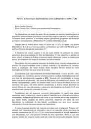
Fig. 1 – Gráfico <strong>de</strong> erros residuais.<br />
40,00000<br />
50,00000<br />
60,00000<br />
Unstan<strong>da</strong>rdized Predicted Value<br />
70,00000<br />
Este gráfico não segue um padrão específico, o que indica que o mo<strong>de</strong>lo é váli<strong>do</strong>.
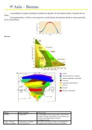
Fig. 2 – Gráfico <strong>da</strong> distribuição <strong>do</strong>s erros.<br />
Observed CumProb<br />
Este gráfico é utiliza<strong>do</strong> p<strong>ar</strong>a verific<strong>ar</strong> se a distribuição <strong>de</strong> probabili<strong>da</strong><strong>de</strong> <strong>do</strong>s erros segue<br />
uma distribuição normal. Uma vez que este se aproxima <strong>de</strong> uma recta, dizemos que segue<br />
uma distribuição normal.
Unstan<strong>da</strong>rdized Residual<br />
40,00000<br />
30,00000<br />
20,00000<br />
10,00000<br />
0,00000<br />
-10,00000<br />
-20,00000<br />
0,00<br />
10,00<br />
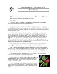
Fig. 3 – Gráfico <strong>do</strong>s erros em função <strong>do</strong> tempo.<br />
Os erros <strong>de</strong> duas observações <strong>de</strong>vem ser in<strong>de</strong>pen<strong>de</strong>ntes. Isto verifica-se através <strong>da</strong> análise<br />
<strong>do</strong> gráfico <strong>da</strong> sequência temporal <strong>do</strong>s resíduos. Não se verifica nenhum tipo <strong>de</strong> padrão e,<br />
então, o mo<strong>de</strong>lo é aceite.<br />
20,00<br />
dia<br />
30,00
Conclusão<br />
Apes<strong>ar</strong> <strong>do</strong> mo<strong>de</strong>lo <strong>de</strong> regressão line<strong>ar</strong> utiliza<strong>do</strong> ser váli<strong>do</strong>, o valor <strong>de</strong> R 2 obti<strong>do</strong> é bastante<br />
baixo (52,4%). A v<strong>ar</strong>iável PM10 está <strong>de</strong>pen<strong>de</strong>nte <strong>do</strong> comportamento <strong>da</strong>s restantes<br />
v<strong>ar</strong>iáveis. O NO2 é o poluente que mais influencia o comportamento <strong>da</strong> PM10 por estas<br />
serem as duas v<strong>ar</strong>iáveis com maior índice <strong>de</strong> correlação
2. Estações <strong>de</strong> Lisboa<br />
Foi-nos possível obter, através <strong>da</strong> matriz <strong>de</strong> cov<strong>ar</strong>iância, um mo<strong>de</strong>lo resultante <strong>de</strong> um<br />
conjunto <strong>de</strong> operações matriciais. O resulta<strong>do</strong> po<strong>de</strong> ser observa<strong>do</strong> na tabela seguinte, on<strong>de</strong><br />
se consi<strong>de</strong>ra a necessi<strong>da</strong><strong>de</strong> <strong>de</strong> que,<br />
Após a introdução inicial <strong>da</strong>s v<strong>ar</strong>iáveis NO, NO2, CO e PM10 no SPSS <strong>de</strong> to<strong>da</strong>s as<br />
estações, introduziram-se as 23 v<strong>ar</strong>iáveis no analyse <strong>da</strong>ta redution factor. Deste mo<strong>do</strong>,<br />
obtivemos a tabela Total V<strong>ar</strong>iance explained, através <strong>da</strong> qual foi possível ver o número <strong>de</strong><br />
componentes através <strong>da</strong> percentagem cumulativa. Constatou-se que apenas eram<br />
necessárias duas componentes p<strong>ar</strong>a “sintetiz<strong>ar</strong>” as v<strong>ar</strong>iáveis, uma vez que, a percentagem<br />
acumula<strong>da</strong> (Cumulative) erea igual ou superior a 75%. No entanto, foram utiliza<strong>da</strong>s 3<br />
componentes, sen<strong>do</strong> a percentagem acumula<strong>da</strong> <strong>de</strong> 86,181.<br />
Tabela 8 – Matriz <strong>da</strong> v<strong>ar</strong>iância explica<strong>da</strong>.<br />
Extraction Method: Principal Component Analysis.<br />
Total V<strong>ar</strong>iance Explained<br />
Initial Eigenvalues Extraction Sums of Squ<strong>ar</strong>ed Loadings<br />
Component Total % of V<strong>ar</strong>iance Cumulative % Total % of V<strong>ar</strong>iance Cumulative %<br />
1 15.962 69.399 69.399 15.962 69.399 69.399<br />
2 2.493 10.841 80.240 2.493 10.841 80.240<br />
3 1.366 5.941 86.181 1.366 5.941 86.181<br />
4 .706 3.069 89.250<br />
5 .444 1.930 91.180<br />
6 .395 1.717 92.898<br />
7 .320 1.393 94.290<br />
8 .278 1.207 95.497<br />
9 .216 .940 96.437<br />
10 .143 .621 97.058<br />
11 .134 .583 97.641<br />
12 .084 .365 98.006<br />
13 .073 .316 98.322<br />
14 .065 .282 98.604<br />
15 .057 .249 98.853<br />
16 .053 .231 99.084<br />
17 .048 .208 99.292<br />
18 .040 .172 99.464<br />
19 .035 .152 99.616<br />
20 .032 .137 99.753<br />
21 .021 .093 99.846<br />
22 .019 .084 99.930<br />
23 .016 .070 100.000
Uma vez que a primeira componente já possui um valor <strong>de</strong> percentagem acumula<strong>da</strong><br />
bastante eleva<strong>do</strong> (69,399%), verifica-se que é a componente que melhor explica, <strong>de</strong> um<br />
mo<strong>do</strong> geral, ca<strong>da</strong> uma <strong>da</strong>s v<strong>ar</strong>iáveis, uma vez que os seus valores próprios gera<strong>do</strong>s pelo<br />
calculo matricial são os mais eleva<strong>do</strong>s, o que se po<strong>de</strong> observ<strong>ar</strong> pelo quadro seguinte, o que<br />
era perfeitamente normal visto os valores próprios (ou a v<strong>ar</strong>iância explica<strong>da</strong> por ca<strong>da</strong><br />
factor) <strong>de</strong>crescerem ao longo <strong>da</strong>s componentes.<br />
Verifica-se ain<strong>da</strong>, pela análise <strong>da</strong> tabela Component Matrix, que a v<strong>ar</strong>iável “pm10_lou” tem<br />
na componente 2 uma melhor explicação.<br />
Tabela 9 - Component Matrix(a)<br />
Component<br />
1 2 3<br />
pm10_lib .804 .533 .102<br />
no_lib .767 -.218 .459<br />
no2_lib .636 .231 .574<br />
co_lib .898 -.072 .160<br />
pm10_ol .774 .477 -.194<br />
no_ol .841 -.381 -.160<br />
no2_ol .913 -.170 .100<br />
co_ol .904 -.146 -.150<br />
pm10_ent .830 .496 -.171<br />
no_ent .874 -.362 -.155<br />
no2_ent .864 -.024 .210<br />
co_ent .922 -.105 -.213<br />
no_rest .833 -.250 .116<br />
no2_rest .838 .001 .481<br />
co_rest .910 .058 .036<br />
pm10_reb .696 .667 -.105<br />
no_reb .814 -.367 -.181<br />
no2_reb .811 -.107 .191<br />
co_reb .922 -.078 -.278<br />
pm10_lou .656 .698 -.148<br />
no_lou .814 -.356 -.266<br />
no2_lou .886 -.126 -.018<br />
co_lou .868 .007 -.235<br />
Extraction Method: Principal Component Analysis.<br />
a 3 components extracted.<br />
Po<strong>de</strong>ríamos elimin<strong>ar</strong> a 3ª componente uma vez que esta apresenta um fraco po<strong>de</strong>r<br />
explicativo, relativamente às restantes. No entanto, e como se po<strong>de</strong> verific<strong>ar</strong> <strong>de</strong> segui<strong>da</strong>,<br />
construiu-se o gráfico que permitiu i<strong>de</strong>ntific<strong>ar</strong> comportamentos semelhantes com esta
componente atrás referi<strong>da</strong>, uma vez que não se verificou qualquer problema inerente à sua<br />
utilização.<br />
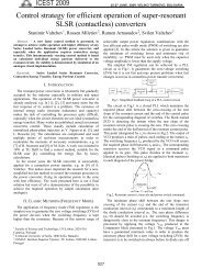
Tal como se po<strong>de</strong> observ<strong>ar</strong> no gráfico, as v<strong>ar</strong>iáveis possuem um comportamento bastante<br />
semelhante uma vez que se encontram bastante concentra<strong>da</strong>s. A v<strong>ar</strong>iável <strong>de</strong> to<strong>da</strong>s as<br />
estações que se encontra ligeiramente mais distancia<strong>da</strong> <strong>da</strong>s restantes é a v<strong>ar</strong>iável p<strong>ar</strong>tículas.<br />
Tal facto po<strong>de</strong> ter ti<strong>do</strong> origem por exemplo na queima <strong>de</strong> combustíveis. As restantes<br />
v<strong>ar</strong>iáveis encontram-se, <strong>de</strong> mo<strong>do</strong> geral, centraliza<strong>da</strong>s num mesmo local, apresentan<strong>do</strong><br />
portanto semelhanças no seu comportamento.<br />
As ligeiras discrepâncias observa<strong>da</strong>s po<strong>de</strong>m est<strong>ar</strong> na origem <strong>da</strong> existência <strong>de</strong> diversos<br />
fluxos <strong>de</strong> tráfego, assim como pela libertação <strong>de</strong>stes compostos liberta<strong>do</strong>s por activi<strong>da</strong><strong>de</strong>s<br />
humanas locais. P<strong>ar</strong>a além <strong>de</strong>stes factos, é importante salient<strong>ar</strong> que, <strong>da</strong><strong>do</strong> ca<strong>da</strong> local ter as<br />
suas condições ambientais específicas, como a presença <strong>de</strong> ventos, gradientes térmicos<br />
entre outros, que po<strong>de</strong>rá ocorrer dispersão <strong>de</strong>stes poluentes na atmosfera.
Component 2<br />
1,0<br />
0,5<br />
0,0<br />
-0,5<br />
-1,0<br />
-1,0<br />
-0,5<br />
0,0<br />
Component 1<br />
Fig. 4 – Gráfico <strong>do</strong>s diferentes componentes.<br />
Component Plot<br />
pm10_lou<br />
pm10_reb<br />
pm10_lib<br />
pm10_ent<br />
pm10_ol<br />
no2_lib co_rest<br />
co_lou<br />
no2_ent co_ent<br />
no2_rest<br />
co_reb<br />
no2_reb<br />
co_olno2_ol<br />
co_lib<br />
no_ol<br />
no_lib<br />
0,5<br />
1,0<br />
1,0<br />
0,5 0,0 -0,5 -1,0<br />
Component 3
Conclusão<br />
Relativamente ao segun<strong>do</strong> objectivo <strong>de</strong>ste trabalho, po<strong>de</strong>mos afirm<strong>ar</strong> que foi alcança<strong>do</strong><br />
com relativo sucesso. Foi-nos possível aperceber, <strong>de</strong> que, <strong>de</strong> um mo<strong>do</strong> geral, existia uma<br />
<strong>de</strong>termina<strong>da</strong> semelhança no comportamento <strong>da</strong>s v<strong>ar</strong>iáveis PM10 entre as diferentes<br />
estações, existin<strong>do</strong> contu<strong>do</strong> uma maior semelhança no comportamento <strong>da</strong>s restantes<br />
v<strong>ar</strong>iáveis.<br />
A existência <strong>de</strong> uma melhor semelhança entre comportamentos verifica<strong>do</strong>s em<br />
<strong>de</strong>termina<strong>da</strong>s estações <strong>de</strong> monitorização, leva-nos a crer que tal facto possa provir <strong>da</strong><br />
existência <strong>de</strong> condições ambientais, tráfego automóvel e veloci<strong>da</strong><strong>de</strong> <strong>de</strong> circulação análogas,<br />
resultan<strong>do</strong> em valores semelhantes <strong>de</strong> ca<strong>da</strong> v<strong>ar</strong>iável.