jj 24 corrente de condução, corrente de deslocamento, equações

24
CORRENTE DE CONDUÇÃO,
CORRENTE DE DESLOCAMENTO,
EQUAÇÕES DE MAXWELL
24.1 - Corrente de Condução e Corrente de Deslocamento
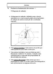
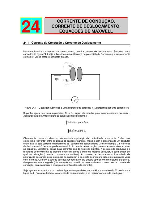
Neste capítulo introduziremos um novo conceito, que é a corrente de deslocamento. Suponha que o
capacitor da figura 24.1 seja submetido a uma diferença de potencial v(t). Sabemos que uma corrente
elétrica i(t) vai se estabelecer neste circuito.
I(t)
S1
Figura 24.1 – Capacitor submetido a uma diferença de potencial v(t), percorrido por uma corrente i(t)
Suponha agora que duas superfícies, S1 e S2, sejam delimitadas pelo mesmo caminho fechado l.
Aplicando a lei de Ampére para as duas superfícies teríamos.
∫
H . dl
= i(
t)
, para S1 e
∫
S2
V(t)
H . dl
= 0 , para S2
Obviamente isto é um absurdo, pois contraria o princípio da continuidade da corrente. É claro que
existe uma “corrente” entre as placas do capacitor paralelo, mesmo sem a presença de um condutor
entre elas. A esta corrente chamaremos de “corrente de deslocamento”. Neste exemplo , a “corrente
de deslocamento” deve se igualar em módulo à corrente de condução, que existe no condutor externo
ao capacitor. Entretanto, essas duas correntes são de natureza distintas. A corrente de condução é o
resultado do movimento de elétrons entre um átomo e outro do material condutor, e pode existir em
qualquer situação (corrente constante ou variável). A corrente de deslocamento é resultado da
polarização de cargas entre as placas do capacitor, e só existe quando a tensão entre as placas varia
com o tempo. Quando a tensão aplicada for constante, ela existirá apenas em um instante transitório,
desaparecendo em seguida (No exemplo em questão o mesmo deverá ocorrer com a corrente de
condução, para satisfazer o princípio da continuidade da corrente).
Seja agora um capacitor e um resistor ligados em paralelos, submetidos a uma tensão V, conforme a
figura 24.2. No capacitor haverá corrente de deslocamento, e no resistor corrente de condução.

Da teoria de circuitos, sabemos que:
e
figura 24.2 – Resistor e capacitor submetidos a tensão V
V
i R =
R
dV
iC = C
dt
onde iR é a corrente de condução no resistor, e iC a corrente de deslocamento no capacitor.
(24.1)
(24.2)
Vamos agora escrever essas relações baseadas em relações de campo, representando os elementos
resistor e capacitor conforme a figura 24.3.
Figura 24.3 – representação do capacitor e do resistor, baseada em grandezas de campo
A intensidade de campo elétrico é a mesma, tanto no resistor como no capacitor, e pode ser expressa
como:
Para o resistor podemos escrever:
ou:
Para o capacitor podemos escrever:
i
V
i R
V
E=
d
V
= = E × d
R 1
σ
i R
= J
A
¡
J R
iR
V E σ E ε
R
= σE
¡
= σE
d
A
iC
(24.3)
(24.4)
(24.5)
(24.6)

ou:
iC = C
dV
dt
A
C= ε
d
(24.7)
(24.8)
V= Ed
(24.9)
A dE
iC = ε d
d dt
iC
dE dD
= J c = ε =
A dt dt
¢
J C
¢
dD
=
dt
(24.10)
(24.11)
(24.12)
£
JC
, a densidade de corrente no capacitor representa uma corrente de deslocamento, que passará a
£
ser representada por Jd
¤
, e JR
¥
condução, que passará a ser representada por J
, a densidade de corrente no resistor representa uma corrente de
.
Suponha agora um meio com as duas características, ao invés de uma resistência pura, em paralelo
com uma capacitância pura (pode ser um mau condutor, ou um dielétrico com perdas). A
generalização da lei de Ampére para esse meio permite escrever:
¦
=
⎛
⎝
∂D
⎞
dS
∂t
⎠
∫ ∫ ⎟ ¦
¦
¦
¦
H.
dL
⎜
J+
Aplicando o teorema de Stokes ao primeiro membro da equação acima, temos:
ou:
§
§
§ ∂D
∇ × H=
J +
∂t
§
§
§ ∂E
∇ × H=
σE+
ε
∂t
(24.13)
(24.14)
(24.15)
O conceito de corrente de deslocamento foi introduzido por J. C. Maxwell, para se levar em conta a
possibilidade de propagação de ondas eletromagnéticas no espaço.
Se o campo elétrico varia harmonicamente com o tempo, as correntes de deslocamento e condução
estão defasadas de 90 graus.
§
§
E = E0
sen ωt
§
§
J = σE0
sen ωt
§
Jd 0
§
= εωE
cosωt
(24.15)
(24.16)
(24.17)

Exemplo 24.1
Um material com σ = 5,0 S/m e εr = 1,0 é submetido a uma intensidade de campo elétrico de
250sen10 10 t V/m. Calcular as densidades de corrente de condução e de deslocamento. Em que
frequência elas terão a mesma amplitude máxima ?
Solução
J
¨
E
cond
Figura 24.4 – dielétrico com perdas
= = σE
= 5 × 250 sen10
10
t
Jcond
1250sen10
=
J
desl
10
t
( A / m
dE
= ε = 8.
85 × 10
dt
Jdesl
= 22.
1cos10
10
t
−12
( A / m
2
)
× 10
Para a mesma amplitude máxima:
σ = εω
2
)
10
× 250 cos10
σ 5. 0
11
ω = =
= 5.
65 × 10 rad / s
−12
ε 8.
85 × 10
w
f = =
2π
Exemplo 24.2
Um capacitor co-axial com raio interno igual a 5 mm, raio externo 6 mm, comprimento de 500 mm
tem um dielétrico com εr = 6,7. Se uma tensão de 250sen377t é aplicada, determine a corrente de
deslocamento e compare-a com a corrente de condução.
Solução
Id(t)
Jcond Jdesl
Figura 24.5 – Capacitor co-axial
Neste exemplo, a corrente entre as placas do
capacitor será do tipo corrente de
deslocamento, e a corrente no condutor
externo corrente de condução. Subentende-se
que o dielétrico é sem perdas.
Da Teoria de circuitos:
dV
ic = C
dt
V(t)
ic(t)
i
c
89.
5
GHz
2πεrε
0l
−
C = = 1.
02 × 10
ln
=
( r r )
0
1.
02 × 10
i
c
1
−9
× 377 ×
−5
= 9.
63×
10
Da teoria eletromagnética:
9
F
250cos
377t
cos377t
O potencial entre as placas do capacitor
obedece à equação de Laplace:
2
∇ V = 0
Em coordenadas cilíndricas, ela se reduz a:
1 ∂ ⎛ dV ⎞
⎜r
⎟ = 0
r ∂r
⎝ dr ⎠
Integrando uma vez em relação a r:
dV
r =
dr
A
A
10
t

Integrando pela segunda vez em relaçao a r:
V = A × ln( r)
+ B
Utilizando as condições de contorno:
e
Resulta:
0 = A × ln 0.
005 + B
250 sen 377t
= A × ln 0.
006 + B
250sen
377t
A =
ln( 0.
006 / 0.
005)
250sen
377t
B =
ln( 0.
005)
ln( 0.
006 / 0.
005)
250sen
377t
V =
ln r +
ln( 0.
006 / 0.
005)
250sen
377t
ln( 0.
005)
ln( 0.
006 / 0.
005)
24.2 – Relações Gerais de Campo
©
E = − ∇V
© 250sen
377t
1
E = −
â r
ln( 0.
006 / 0.
005)
r
©
J
d
©
Jd ©
dE
= ε
dt
−6
30.
6 × 10
= −
r
i
d
id = Jd
× S
cos 377tâ
−5
= − 9.
63 × 10
o que comprova que a corrente de
deslocamento, dentro do capacitor, é igual à
corrente de condução, no condutor externo. O
sinal menos obtido não afeta a nossa
resposta, pois é fruto de arbitrariedades ao se
impor direções e condições de contorno.
Em ocasião anterior foi mostrado que a divergência do campo magnético é nula, ou seja :
∇ •
B = 0
E do calculo vetorial, sabe-se que a seguinte relação é válida, para qualquer função vetorial F :
∇ •
( ∇ × F ) = 0
Ficando demonstrada a existência de um vetor potencial magnético A , tal que :
B = ∇ ×
Por outro lado, a lei da Faraday expressa na forma pontual é :
∇ ×
E
= −
Substituindo (24.20 ) em ( 24.21), teremos, portanto :
Ou :
∇ ×
E
= −
∂
A
∂B
∂t
( ∇ × A)
∂t
A
r
(24.18)
(24.19)
(24.20)
(24.21)
(24.22)

⎛ ∂A
⎞
∇ × ⎜E
⎟
⎜
+ = 0
t ⎟
⎝ ∂ ⎠
Desde que o rotacional da expressão entre parêntesis é igual a zero, ela deve ser igual ao gradiente
de uma função escalar. Assim, podemos escrever :
∂A
E + = ∇f
∂t
(24.23)
(24.24)
Onde f é uma função escalar. Fazendo f = −V
, o vetor intensidade pode ser escrito de uma forma
generalizada, servindo tanto para campos elétricos variantes no tempo, como para campos elétricos
estáticos :
∂A
E = − ∇V
−
∂t
(24.25)
Relembrando, as expressões clássicas para o potencial escalar eletrostático, e para o vetor potencial
magnético são, respectivamente :
∫ ρ 1
V = dv
(24.26)
4πε
v
0 R
Em termos da Equação de Poisson, temos :
Para campos elétricos e :
Para campos magnéticos lineares
∇
2
A =
A
µ
4π
∫
v
J
dv
R
∇ V = −
ρ
ε
2
⎛
= µ ⎜−
J
⎝
24.3 - As Equações de Maxwell para Campos Variáveis no Tempo.
− σ
∂A
∂t
⎞
⎟
⎠
(24.27)
(24.28)
(24.29)
No capítulo 15 estabelecemos as 4 equações de Maxwell para campos elétricos e magnéticos
estáticos (invariantes no tempo). Elas podem ser escrito tanto na forma integral:
∫ H.
dL=
∫
∫
s
l s
JdS
E.
dL=0
∫
∫
D.
dS=
ρdV
v
∫ B.
dS=
0
s
(24.30)
(24.31)
(24.32)
(24.33)

Ou na forma diferencial :
∇ × H=
J
∇×
E= 0
∇. D=
ρ
∇.
B=
0
(24.34)
(24.35)
(24.36)
(24.37)
As 4 equações de Maxwell podem também ser escritas, considerando-se campos elétricos e
magnéticos variáveis no tempo. Na forma diferencial temos:
E na forma diferencial :
=
⎛
⎝
∂D
⎞
dS
∂t
⎠
∫ ∫ ⎟
H.
dL
⎜
J +
∂B
= dS
t
∫ E.
dL
− ∫ ∂
∫
s
∫
D.
dS=
ρdV
v
∫ B.
dS=
0
s
∂D
∇ × H=
J+
∂t
∂B
∇ × E=
−
∂t
∇. D=
ρ
∇.
B=
0
(24.38)
(24.39)
(24.40)
(24.41)
(24.42)
(24.43)
(24.44)
(24.45)
Observe que a 3ª e 4ª equação não mudam em relação aos campos estáticos. A segunda equação
corresponde à lei de Faraday, considerando efeito variacional da tensão induzida.
24.2-1 - Equações de Maxwell no Espaço Livre
Quando Maxwell formulou as suas equações, a sua maior preocupação era demonstrar a existência
de ondas eletromagnéticas se propagando no espaço livre. Neste caso, não existirá corrente de
condução, nem densidades de cargas livres. Assim as equações podem ser simplificadas:
∂D
= dS
t
∫ H.
dL
∫ ∂
(24.46)

E na forma diferencial:
ou:
∂B
= dS
t
∫ E.
dL
− ∫ ∂
∫
s
D.
dS=
0
∫ B.
dS=
0
s
∂D
∇×
H= ∂t
∂B
∇ × E=
−
∂t
∇.
D=
0
∇.
B=
0
∂E
∇ × H= ε0
∂t
∂H
∇ × E= − µ 0
∂t
∇.
E=
0
∇.
H=
0
24.2.-2 Equações de Maxwell para Campos Variantes Harmonicamente com o Tempo
(24.47)
(24.48)
(24.49)
(24.50)
(24.51)
(24.52)
(24.53)
(24.54)
(24.55)
(24.56)
(24.57)
Finalmente apresentamos as formulações das equações de Maxwell para campos eletromagnéticos
que variam harmonicamente com o tempo (não necessariamente o espaço livre). Considerando uma
variação do tipo e jwt , elas podem ser escritas como:
E na forma diferencial
∫ H.
dL=
( σ+
jωε)
∫
s s
∫ E.
dL=
− jωµ
∫
l s
∫
∫
EdS
HdS
D.
dS=
ρdV
v
s
∫ B.
dS=
0
s
∇
× H=
( σ+
jωε)E
(24.59)
(24.60)
(24.61)
(24.62)

∇ × E=
− jωµ
H
∇.
D=
0
∇.
B=
0
Deste último grupo de equações partiremos para formular a equação de onda eletromagnética.
EXERCÍCIOS
(24.63)
(24.64)
(24.65)
(24.66)
1)- Conhecida a densidade de corrente de condução num dielétrico dissipativo,Jc 0,02 sen i0 9 t(A/m 2 ),
encontre a densidade de corrente de deslocamento se σ 10 3 Sim e ε = 6,5.
1,15x10 -6 cos10 -9 t (A/m 2 )
2)- Um condutor de seção reta circular de 1,5 mm de raio suporta uma corrente ic = 5,5 sen4x10 10 t
(µA). Quanto vale a amplitude da densidade de corrente de deslocamento, se σ = 35 MS/m εr = 1
7,87x10 -3 µA/m 2
3)- Descubra a freqüência para a qual as densidades de corrente de condução e deslocamento são
idênticas em (a) água destilada, onde σ = 2,0×10 -4 S/m, εr = 81; (b) água salgada, onde σ= 4,0
S/m e εr = 1.
(a) 4,44 x 104 Hz;(b) 7,19 x 1010 Hz
4)- Duas cascas esféricas condutoras concêntricas com raios r1 = 0,5 mm e r2 = 1 mm, acham-se
separadas por um dielétrico de εr = 8,5. Encontre a capacitância e calcule ic dada uma tensão
aplicada v = 150sen5000t(V). Calcule a corrente de deslocamento iD e compare-a com ic.
ic = iD = 7,09×10-7cos5000t (A)
5)- Duas placas condutoras planas e paralelas de área 0,05 m 2 acham-se separadas por 2 mm de um
dielétrico com perdas com εr= 8,3 e σ = 8,0×10 -4 S/m. Aplicada uma tensão v = 10 sen 10 7 t (V),
calcule o valor rms da corrente total.
0,192 A
6)- Um capacitor de placas paralelas, separadas por 0,6 mm e com um dielétrico de εr = 15,3 tem uma
tensão aplicada de rms 25 V na frequência de 15 GHz. Calcule o rms da densidade de corrente de
deslocamento. Despreze o espraiamento.
5,32×105 A/m2