a synchronized learning algorithm for nonlinear part in a lattice ...

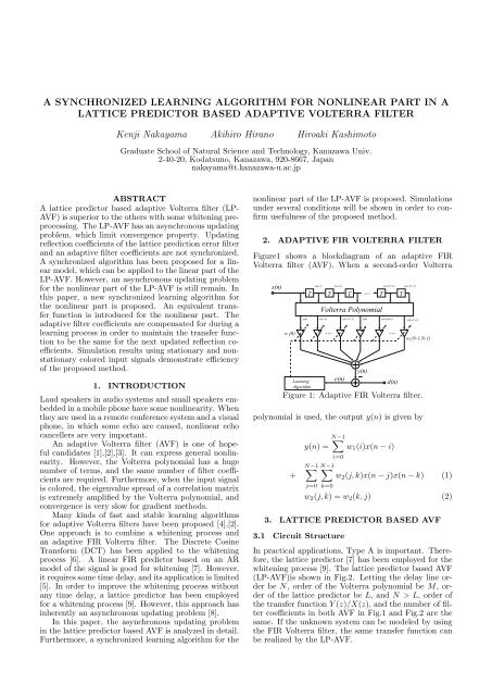
Output Error[dB]parts. The learning curve of ’Synchronized(L)’ is almostthe same as that of ’Asynchronous’. On the contrary,the synchronized learning algorithm for both the linearand nonlinear parts, shown with ’Synchronized(L+NL)’,can improve the learning curve by 15dB.Figure7 shows the learning curves for the nonstationarycolored signal, which is generated through the2nd-order AR model, whose pole oscillates around π/4by ±20% with a period of 500 samples. In this case,also the synchronized learning algorithm for both thelinear and nonlinear parts is superior to the others. Inthis figure, ’Synchronized(L)’ is not shown, because it isalmost the same as ’Asynchronous’.Furthermore, the learning curves for another nonstationarycolored signal are shown in Fig.8. The poleof the 2nd-order AR model oscillates around π/4 by±100% with a period of 500 samples. In this case, thereflection coefficients change more rapidly compared tothe previous example. For this reason, the convergencebecomes a little slower than the previous. Still, the synchronizedlearning algorithm can improve the convergenceproperty.100-10-20-30-40-50-60-70Synchronized(L)Synchronized(L+NL)Asynchronous-800 20000 40000 60000 80000 100000 120000 140000 160000 180000 200000Iteration[sample]Figure 6: Learning curves for LP-AVF using stationarycolored signal. Synchronized(L) and Synchronized(L+NL)means synchronized learning algorithmsfor linear part and linear and nonlinear parts, respectively,are used.Output Error[dB]100-10-20-30-40-50-60-70-800 20000 40000 60000 80000 100000 120000 140000 160000 180000 200000Iteration[sample]AsynchronousSynchronized(L+NL)Figure 7: Learning curves for LP-AVF using nonstationarycolored signal. Pole of 2nd-order AR model oscillatesaround π/4 by 20% with period 500 samples.Output Error[dB]0-10-20-30-40-50-60-70Synchronized(L+NL)-800 20000 40000 60000 80000 100000 120000 140000 160000 180000 200000Iteration[sample]AsynchronousFigure 8: Learning curves for LP-AVF using nonstationarycolored signal. Pole of 2nd-order AR model oscillatesaround π/4 by 100% with period of 500 samples.6. CONCLUSIONSSeveral kinds of whitening methods for the adaptiveVolterra filter have been compared. The lattice predictorbased AVF is superior to the others. Convergenceproperty of the asynchronous LP-AVF has beenanalyzed. Furthermore, the synchronized learning algorithmfor the nonlinear part of the LP-AVF has beenproposed, and its usefulness has been confirmed throughseveral simulations using stationary and nonstationarycolored signals.REFERENCES[1] V. J. Mathews, ”Adaptive polynomial filters,” IEEESignal Processing Mag., pp. 10-26, July 1991.[2] A.Stenger, L.Trautmann and R.Rabenstein, ”Nonlinearacoustic echo cancellation with 2nd order adaptiveVolterra filters,” IEEE Proc. ICASSP’99, AE1.7,pp877-880, 1999.[3] B.S.Nollett and D.L.Jones, ”Nonlinear echo cancellationfor hands-free speakerphones,” 1997 IEEE Workshopon Nonlinear Signal and Image Proc[4] J.Lee and V.J.Mathews, ”A fast recursive least squaresadaptive second order Volterra filter and its performanceanalysis,”IEEE Trans on Signal Processing,Vol.41, No.3, pp.1087-1102, Mar 1993.[5] A.Strenger and W.Kellermann, ”Nonlinear acousticecho cancellation with fast converging memoryless preprocessor,”Proc. IEEE Workshop on Acoustic Echoand Noise Control, Pocono Manor, PA, USA, September,1999.[6] X.Li and W.K.Jenkins, ”Computationally efficient algorithmsfor third order adaptive Volterra filters,” IEEEProc. ICASSP’98, DSP5.3, 1998.[7] S.Haykin, Adaptive Filter Theory, 3rd Ed., PrenticeHall Inc., New York, 1996.[8] N.Tokui, K.Nakayama and A.Hirano, ”A synchronizedlearning algorithm for reflection coeffcients and tapweights in a joint lattice predictor and transversalfilter”, IEEE Proc. ICASSP’2001, Salt Lake City,pp.1472-1475, May 2001.[9] K.Nakayama, A.Hirano and H.Kashimoto,”A latticepredictor based adaptive Volterra filter and a synchronizedlearning algorithm”, Proc., XII Europian SignalProcessing Conference, Vienna, Austria, pp.1585-1588,Sept. 2004.