Aplicaciones de la integral.
Aplicaciones de la integral.
Aplicaciones de la integral.

Create successful ePaper yourself
Turn your PDF publications into a flip-book with our unique Google optimized e-Paper software.
12.1 Áreas <strong>de</strong> superficies p<strong>la</strong>nas.<br />
12.1.1 Funciones dadas <strong>de</strong> forma explícita.<br />
Tema 12<br />
<strong>Aplicaciones</strong> <strong>de</strong> <strong>la</strong> <strong>integral</strong>.<br />
A <strong>la</strong> vista <strong>de</strong>l estudio <strong>de</strong> <strong>la</strong> <strong>integral</strong> <strong>de</strong>finida realizado en el Tema 10, parece razonable <strong>la</strong> siguiente<br />
<strong>de</strong>finición:<br />
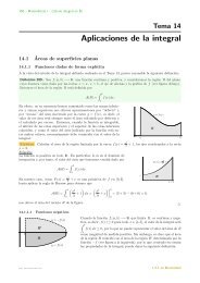
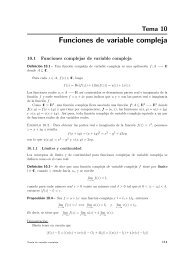
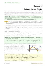
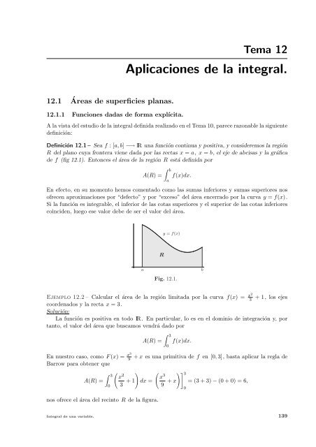
Definición 12.1 – Sea f : [a, b] −→ IR una función continua y positiva, y consi<strong>de</strong>remos <strong>la</strong> región<br />
R <strong>de</strong>l p<strong>la</strong>no cuya frontera viene dada por <strong>la</strong>s rectas x = a, x = b, el eje <strong>de</strong> abcisas y <strong>la</strong> gráfica<br />
<strong>de</strong> f (fig 12.1). Entonces el área <strong>de</strong> <strong>la</strong> región R está <strong>de</strong>finida por<br />
b<br />
A(R) = f(x)dx.<br />
a<br />
En efecto, en su momento hemos comentado como <strong>la</strong>s sumas inferiores y sumas superiores nos<br />
ofrecen aproximaciones por “<strong>de</strong>fecto” y por “exceso” <strong>de</strong>l área encerrado por <strong>la</strong> curva y = f(x).<br />
Si <strong>la</strong> función es integrable, el inferior <strong>de</strong> <strong>la</strong>s cotas superiores y el superior <strong>de</strong> <strong>la</strong>s cotas inferiores<br />
coinci<strong>de</strong>n, luego ese valor <strong>de</strong>be <strong>de</strong> ser el valor <strong>de</strong>l área.<br />
R<br />
y = f(x)<br />
a b<br />
Fig. 12.1.<br />
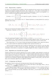
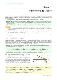
Ejemplo 12.2 – Calcu<strong>la</strong>r el área <strong>de</strong> <strong>la</strong> región limitada por <strong>la</strong> curva f(x) = x2<br />
3 + 1, los ejes<br />
coor<strong>de</strong>nados y <strong>la</strong> recta x = 3.<br />
Solución:<br />
La función es positiva en todo IR. En particu<strong>la</strong>r, lo es en el dominio <strong>de</strong> integración y, por<br />
tanto, el valor <strong>de</strong>l área que buscamos vendrá dado por<br />
3<br />
A(R) = f(x)dx.<br />
0<br />
En nuestro caso, como F (x) = x3<br />
9 + x es una primitiva <strong>de</strong> f en [0, 3], basta aplicar <strong>la</strong> reg<strong>la</strong> <strong>de</strong><br />
Barrow para obtener que<br />
<br />
3 x2 x3 3<br />
A(R) = + 1 dx = + x = (3 + 3) − (0 + 0) = 6,<br />
3 9<br />
nos ofrece el área <strong>de</strong>l recinto R <strong>de</strong> <strong>la</strong> figura.<br />
0<br />
Integral <strong>de</strong> una variable. 139<br />
0
1<br />
f(x)= x2<br />
3 +1<br />
R<br />
x=3<br />
12.1 Áreas <strong>de</strong> superficies p<strong>la</strong>nas.<br />
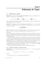
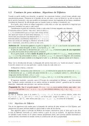
Cuando <strong>la</strong> función f : [a, b] −→ IR que limita R, es continua y negativa, es <strong>de</strong>cir, f(x) ≤ 0,<br />
b<br />
para todo x ∈ [a, b], se tiene que f(x)dx ≤ 0, por lo que este valor no representa el área <strong>de</strong><br />
a<br />
R como magnitud <strong>de</strong> medida positiva. Sin embargo, es c<strong>la</strong>ro que el área <strong>de</strong> <strong>la</strong> región R coinci<strong>de</strong><br />
con el área <strong>de</strong> <strong>la</strong> región R ′ <strong>de</strong>terminada por <strong>la</strong> función −f (fig 12.2), por lo que, teniendo en<br />
R<br />
R<br />
y = −f(x)<br />
a b<br />
Fig. 12.2.<br />
y = f(x)<br />
cuenta <strong>la</strong>s propieda<strong>de</strong>s <strong>de</strong> <strong>la</strong> <strong>integral</strong>, pue<strong>de</strong> darse <strong>la</strong> siguiente <strong>de</strong>finición.<br />
Definición 12.3 – Sea f : [a, b] −→ IR una función continua y negativa. Consi<strong>de</strong>remos <strong>la</strong> región<br />
R <strong>de</strong>l p<strong>la</strong>no cuya frontera viene dada por <strong>la</strong>s rectas x = a, x = b, el eje <strong>de</strong> abcisas y <strong>la</strong> gráfica<br />
<strong>de</strong> f . Entonces el área <strong>de</strong> <strong>la</strong> región R está <strong>de</strong>finida por<br />
b<br />
b<br />
A(R) = −f(x)dx = − f(x)dx.<br />
a<br />
Observación 12.4 – Es c<strong>la</strong>ro entonces que para calcu<strong>la</strong>r el área <strong>de</strong> regiones p<strong>la</strong>nas <strong>de</strong>be analizarse<br />
el signo <strong>de</strong> <strong>la</strong> función en el intervalo <strong>de</strong> integración. De no hacerlo así, <strong>la</strong> parte negativa <strong>de</strong> <strong>la</strong><br />
función “restará” el área que encierra <strong>de</strong>l área encerrado por <strong>la</strong> parte positiva.<br />
Contraejemplo.- Hal<strong>la</strong>r el área encerrado por <strong>la</strong> función f(x) = sen x, en el intervalo [0, 2π].<br />
2π<br />
2π El valor sen xdx = − cos x = (− cos(2π)) − (− cos 0) = 0, es c<strong>la</strong>ro que no representa<br />
0<br />
el área encerrada por <strong>la</strong> curva.<br />
0<br />
R1<br />
a<br />
π 2π<br />
R2<br />
Ahora bien, teniendo en cuenta que <strong>la</strong> función sen x es positiva en [0, π] y negativa en [π, 2π],<br />
el valor real <strong>de</strong>l área encerrado será por tanto<br />
π<br />
2π<br />
A(R) = A(R1) + A(R2) = sen xdx +<br />
0<br />
π<br />
π 2π − sen xdx = − cos x + cos x = 2 + 2 = 4.<br />
0 π<br />
Integral <strong>de</strong> una variable. 140
12.1 Áreas <strong>de</strong> superficies p<strong>la</strong>nas.<br />
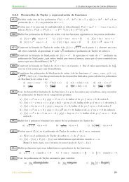
Ejemplo 12.5 – Hal<strong>la</strong>r el área <strong>de</strong>terminada por <strong>la</strong> curva f(x) = (x−1)(x−2), <strong>la</strong>s rectas x = 0,<br />
x = 5<br />
2 y el eje <strong>de</strong> abcisas.<br />
Solución:<br />
f(x) es menor o igual a cero en [1, 2] y positiva en el resto. Luego<br />
Como F (x) = x3<br />
3<br />
− 3x2<br />
2<br />
2<br />
1<br />
A(R) =<br />
0<br />
R1<br />
f(x)=(x−1)(x−2)<br />
R2<br />
R3<br />
1 2 2.5<br />
2<br />
f(x)dx + −f(x)dx +<br />
1<br />
5<br />
2<br />
+ 2x es una primitiva <strong>de</strong> f(x) en [0, 5<br />
2 ],<br />
2<br />
f(x)dx.<br />
A(R) = (G(1) − G(0)) − (G(2) − G(1)) + (G( 5<br />
5−4+5+5−4<br />
2 ) − G(2)) = 6 = 7<br />
6 .<br />
En <strong>la</strong>s <strong>de</strong>finiciones anteriores pue<strong>de</strong> consi<strong>de</strong>rarse, que el área calcu<strong>la</strong>do esta encerrado por<br />
<strong>la</strong> función y = f(x) y <strong>la</strong> función y = 0, cuando <strong>la</strong> f es positiva, y por <strong>la</strong> función y = 0 y <strong>la</strong><br />
función y = f(x), cuando <strong>la</strong> f es negativa. En ambos casos, se tiene que<br />
b<br />
A(R) =<br />
a<br />
b b<br />
b b<br />
b<br />
f(x)dx− 0dx = (f(x)−0)dx y A(R) = 0dx− f(x)dx = (0−f(x))dx,<br />
a<br />
a<br />
a a<br />
a<br />
es <strong>de</strong>cir, que el área encerrado por ambas funciones es <strong>la</strong> <strong>integral</strong> <strong>de</strong> <strong>la</strong> función mayor menos <strong>la</strong><br />
<strong>integral</strong> <strong>de</strong> <strong>la</strong> función menor. En general, se tiene entonces que<br />
Si f, g : [a, b] −→ IR son funciones continuas, con f(x) ≥ g(x) para todo x ∈ [a, b]. Entonces,<br />
si R es <strong>la</strong> región <strong>de</strong>l p<strong>la</strong>no cuya frontera viene dada por <strong>la</strong>s rectas x = a, x = b, el eje <strong>de</strong> abcisas<br />
y <strong>la</strong>s gráficas <strong>de</strong> f y g , el área <strong>de</strong> R se obtiene como<br />
b<br />
A(R) =<br />
a<br />
b<br />
f(x)dx − g(x)dx =<br />
a<br />
b<br />
a<br />
<br />
<br />
f(x) − g(x) dx.<br />
En efecto, si <strong>la</strong>s funciones verifican que 0 ≤ g(x) ≤ f(x), es c<strong>la</strong>ro que el área encerrado por f<br />
y g es el área encerrado por f menos el área encerrado por g (fig. 12.3), es <strong>de</strong>cir,<br />
b<br />
A(Rf−g) = A(Rf ) − A(Rg) =<br />
a<br />
b<br />
f(x)dx − g(x)dx.<br />
a<br />
Si alguna <strong>de</strong> el<strong>la</strong>s toma valores negativos, el área entre ambas, R, es el mismo que si le sumamos<br />
a cada función una constante C que <strong>la</strong>s haga positivas y, por tanto, el área R es el área R ′<br />
encerrado por f + C menos el área encerrado por g + C (fig. 12.3), es <strong>de</strong>cir,<br />
b<br />
b<br />
A(Rf−g) = A(Rf+C) − A(Rg+C) = (f(x) + C)dx − (g(x) + C)dx<br />
Observaciones 12.6 –<br />
a<br />
a<br />
b b b b b<br />
= f(x)dx + Cdx − g(x)dx − Cdx =<br />
a<br />
a<br />
a<br />
a<br />
a<br />
b<br />
f(x)dx − g(x)dx.<br />
a<br />
Integral <strong>de</strong> una variable. 141
y = f(x)+C<br />
y = f(x)<br />
R<br />
y = g(x)+C<br />
R<br />
a y = g(x) b<br />
Fig. 12.3.<br />
12.1 Áreas <strong>de</strong> superficies p<strong>la</strong>nas.<br />
⋆ Las <strong>de</strong>finiciones son ampliables para a = −∞ y/ó b = +∞ cuando tenga sentido, es<br />
<strong>de</strong>cir, cuando <strong>la</strong>s <strong>integral</strong>es impropias correspondientes sean convergentes.<br />
⋆ De forma análoga, si <strong>la</strong> región está limitada por funciones x = f(y), x = g(y) y <strong>la</strong>s<br />
rectas y = c e y = d, siendo g(y) ≤ f(y) para todo y ∈ [c, d], el área <strong>de</strong> <strong>la</strong> región pue<strong>de</strong><br />
encontrarse mediante <strong>la</strong> fórmu<strong>la</strong><br />
d<br />
A(R) =<br />
c<br />
<br />
<br />
f(y) − g(y) dy.<br />
Ejemplo.- Calcu<strong>la</strong>r el área <strong>de</strong> <strong>la</strong> región acotada comprendida entre <strong>la</strong>s parábo<strong>la</strong>s <strong>de</strong><br />
ecuaciones y 2 + 8x = 16 e y 2 − 24x = 48.<br />
x=f(y)<br />
√ 24<br />
R<br />
− √ 24<br />
x=g(y)<br />
Las parábo<strong>la</strong>s pue<strong>de</strong>n escribirse como x = g(y) = 16−y2<br />
8<br />
<strong>de</strong> corte <strong>de</strong> ambas parábo<strong>la</strong>s son <strong>la</strong>s soluciones <strong>de</strong> <strong>la</strong> ecuación<br />
16 − y 2<br />
8<br />
= y2 − 48<br />
24 =⇒ y = ±√ 24.<br />
Como en el intervalo [− √ 24, √ 24] es f(y) ≤ g(y), se tiene que<br />
<br />
A(R) =<br />
√ 24<br />
− √ 24<br />
16−y 2<br />
8<br />
<br />
dy −<br />
√ 24<br />
− √ 24<br />
y x = f(y) = y2 −48<br />
24 . Los puntos<br />
y2 <br />
−48<br />
dy =<br />
24 √ 24<br />
− √ <br />
4−<br />
24<br />
y2<br />
<br />
dy = 4y−<br />
6<br />
y3<br />
<br />
18<br />
√ 24<br />
− √ 24<br />
= 16√<br />
24.<br />
3<br />
Integral <strong>de</strong> una variable. 142
12.1.2 Funciones dadas <strong>de</strong> forma paramétrica.<br />
12.1 Áreas <strong>de</strong> superficies p<strong>la</strong>nas.<br />
Estudiaremos ahora el caso en que <strong>la</strong> curva y = f(x) en [a, b] viene dada por <strong>la</strong>s ecuaciones<br />
paramétricas. <br />
x = ϕ(t)<br />
y = ψ(t) .<br />
Si f es positiva (si f es negativa o cambia <strong>de</strong> signo se escribirá lo correspondiente), el área<br />
encerrado por f es<br />
b<br />
A(R) = f(x)dx.<br />
Como x = ϕ(t) e y = ψ(t) tenemos que<br />
a<br />
y = f(x) = f(ϕ(t)) = ψ(t) y dx = ϕ ′ (t)dt,<br />
luego usando este cambio <strong>de</strong> variable en <strong>la</strong> <strong>integral</strong>, se tiene que<br />
b<br />
t2<br />
A(R) = f(x)dx = f(ϕ(t))ϕ ′ t2<br />
(t)dt = ψ(t)ϕ ′ (t)dt,<br />
a<br />
t1<br />
don<strong>de</strong> ϕ(t1) = a y ϕ(t2) = b. En consecuencia, pue<strong>de</strong> calcu<strong>la</strong>rse el área encerrado por <strong>la</strong><br />
curva dada en paramétricas usando estas ecuaciones, –naturalmente teniendo en cuenta el signo<br />
<strong>de</strong> y = ψ(t)–.<br />
Observación:<br />
Los extremos <strong>de</strong> integración t1 y t2 aparecen al efectuar el cambio <strong>de</strong> variable, y están asociados<br />
respectivamente a a y b, con a ≤ b, por lo que pue<strong>de</strong> ser tanto t1 ≤ t2 como t1 ≥ t2 según el<br />
caso (<strong>de</strong> hecho y respectivamente, según que el signo <strong>de</strong> x ′ = ϕ ′ (t) sea positivo o negativo en el<br />
intervalo).<br />
<br />
x = cos t<br />
Ejemplo 12.7 – Hal<strong>la</strong>r el área encerrado por <strong>la</strong> curva<br />
, con t ∈ [0, 2π].<br />
y = sen t<br />
Solución:<br />
El área pedida, es el área <strong>de</strong>l círculo <strong>de</strong> radio 1. Cuando y ≥ 0, haciendo el cambio x = cos t,<br />
para el cuál dx = − sen tdt con 1 = cos 0 y −1 = cos π , tenemos que<br />
1<br />
0<br />
π<br />
A(R+) = y(x)dx = sen t(− sen t)dt = sen 2 π<br />
tdt =<br />
−1<br />
−1<br />
π<br />
π<br />
0<br />
π<br />
t1<br />
0<br />
1 − cos 2t<br />
dt =<br />
2<br />
π<br />
2<br />
Cuando y ≤ 0, con el mismo cambio se obtiene 1 = cos 2π y −1 = cos π , <strong>de</strong> don<strong>de</strong><br />
1<br />
2π<br />
2π<br />
A(R−) = − y(x)dx = − sen t(− sen t)dt = sen 2 tdt = t<br />
2π sen 2t<br />
− =<br />
2 4<br />
π<br />
2<br />
Observación 12.8 – El ejemplo anterior subraya el comentario hecho en <strong>la</strong> observación pre-<br />
via sobre los extremos <strong>de</strong> integración. Si, directamente, <strong>de</strong>cimos que el valor <strong>de</strong> A(R+) es<br />
π<br />
sen t(− sen t)dt estamos cometiendo un error, pues esta <strong>integral</strong> se obtiene <strong>de</strong><br />
0<br />
π<br />
−1<br />
sen t(− sen t)dt = y(x)dx<br />
0<br />
1<br />
y el valor calcu<strong>la</strong>do no es el <strong>de</strong>l área, sino<br />
π<br />
−1<br />
1<br />
sen t(− sen t)dt = y(x)dx = − y(x)dx = −A(R+).<br />
0<br />
1<br />
−1<br />
Téngase presente, que si bien en este caso es c<strong>la</strong>ro que basta con cambiar el signo para obtener<br />
el valor buscado, en general, pue<strong>de</strong>n aparecer varios términos en el cálculo <strong>de</strong>l área <strong>de</strong> forma<br />
que el resultado final no haga sospechar el error cometido.<br />
Integral <strong>de</strong> una variable. 143<br />
π
12.1.3 Funciones dadas <strong>de</strong> forma po<strong>la</strong>r.<br />
Por último estudiaremos el caso <strong>de</strong> curvas dadas en coor<strong>de</strong>nadas po<strong>la</strong>res.<br />
Consi<strong>de</strong>remos una curva dada en coor<strong>de</strong>nadas po<strong>la</strong>res por <strong>la</strong> ecuación<br />
r = f(θ)<br />
12.1 Áreas <strong>de</strong> superficies p<strong>la</strong>nas.<br />
don<strong>de</strong> f es continua y sea S el sector comprendido entre los ángulos θ = α, θ = β y <strong>la</strong><br />
gráfica <strong>de</strong> <strong>la</strong> función. Con un <strong>de</strong>sarrollo análogo al realizado en <strong>la</strong> construcción <strong>de</strong> <strong>la</strong> <strong>integral</strong><br />
<strong>de</strong>finida para funciones dadas explícitamente, po<strong>de</strong>mos <strong>de</strong>finir sumas superiores e inferiores y <strong>la</strong><br />
integrabilidad, a través <strong>de</strong> particiones <strong>de</strong>l intervalo angu<strong>la</strong>r [α, β] consi<strong>de</strong>rando <strong>la</strong>s áreas <strong>de</strong> los<br />
correspondientes sectores circu<strong>la</strong>res (el área <strong>de</strong> un sector circu<strong>la</strong>r <strong>de</strong> radio r y ángulo θ viene<br />
dado por θ<br />
2 r2 ), como pue<strong>de</strong> observarse en <strong>la</strong> figura 12.4.<br />
β α<br />
Fig. 12.4.<br />
r =f(θ)<br />
La expresión <strong>de</strong>l área mediante una <strong>integral</strong> en función <strong>de</strong>l ángulo, se obtiene <strong>de</strong> forma más<br />
intuitiva si consi<strong>de</strong>ramos <strong>la</strong>s sumas <strong>de</strong> Riemman asociadas a este proceso <strong>de</strong> integración, es <strong>de</strong>cir,<br />
dada una partición <strong>de</strong> [α, β], P = {α = θ0, θ1, . . . , θn−1, θn = β}, y cualquier elección <strong>de</strong> E ,<br />
tenemos que<br />
n<br />
2 △θi<br />
S(f, Pn, E) = (f(ei))<br />
2<br />
i=1<br />
Hemos pues, introducido <strong>la</strong> siguiente <strong>de</strong>finición:<br />
luego, tomando particiones<br />
cada vez más finas<br />
→<br />
β<br />
α<br />
2 dθ<br />
(f(θ))<br />
2 .<br />
Definición 12.9 – Sea f: [α, β] −→ IR continua. El área <strong>de</strong> <strong>la</strong> región S <strong>de</strong>l p<strong>la</strong>no limitada por<br />
<strong>la</strong> curva r = f(θ) y <strong>la</strong>s rectas que forman un ángulo α y un ángulo β con el eje se abcisas<br />
positivo, (fig. 12.5), viene dada por <strong>la</strong> <strong>integral</strong><br />
A(S) = 1<br />
β<br />
f<br />
2 α<br />
2 (θ)dθ. 〈12.1〉<br />
Si r = f(θ) y r = g(θ) son dos curvas dadas en coor<strong>de</strong>nadas po<strong>la</strong>res, don<strong>de</strong> f, g : [α, β] −→ IR<br />
son continuas con g(θ) ≤ f(θ), para todo θ ∈ [α, β] y S es el sector comprendido entre los<br />
ángulos θ1 = α, θ2 = β y <strong>la</strong>s gráficas <strong>de</strong> <strong>la</strong>s funciones r = f(θ) y r = g(θ) (fig. 12.6), se tendrá<br />
que<br />
A(S) = 1<br />
β<br />
f<br />
2 α<br />
2 (θ)dθ − 1<br />
b<br />
g<br />
2 a<br />
2 (θ)dθ = 1<br />
β <br />
f<br />
2 a<br />
2 (θ) − g 2 <br />
(θ) dθ.<br />
Integral <strong>de</strong> una variable. 144
β<br />
β<br />
α<br />
S<br />
Fig. 12.5.<br />
r =g(θ)<br />
α<br />
Fig. 12.6.<br />
r =f(θ)<br />
r =f(θ)<br />
S<br />
12.1 Áreas <strong>de</strong> superficies p<strong>la</strong>nas.<br />
Observación 12.10 – También pue<strong>de</strong> llegarse a <strong>la</strong> fórmu<strong>la</strong> 〈12.1〉 mediante razonamientos geométricos<br />
y un cambio <strong>de</strong> variable sobre <strong>la</strong> <strong>integral</strong> en coor<strong>de</strong>nadas cartesianas.<br />
Si observamos <strong>la</strong> figura 12.5 –y supuesto por comodidad que para cada valor <strong>de</strong> x no existe<br />
más que un valor <strong>de</strong> y –, en coor<strong>de</strong>nadas cartesianas <strong>la</strong> función r = f(θ), se expresa por<br />
y = f(θ) sen θ<br />
, con θ ∈ [α, β], luego x ∈ [f(β) cos β, f(α) cos α].<br />
x = f(θ) cos θ<br />
Así mismo, <strong>la</strong> recta <strong>de</strong> ángulo α tiene por expresión yα = (tg α)x, cuando x ∈ [0, f(α) cos α],<br />
y <strong>la</strong> recta <strong>de</strong> ángulo β , yβ = (tg β)x, cuando x ∈ [0, f(β) cos β]. Por tanto, el área <strong>de</strong> S será el<br />
área encerrado por <strong>la</strong>s gráficas <strong>de</strong> <strong>la</strong>s funciones <strong>de</strong> x, es <strong>de</strong>cir,<br />
A(S) =<br />
f(β) cos β<br />
0<br />
Calcu<strong>la</strong>ndo directamente I1 e I3 , se tiene que<br />
f(β) cos β<br />
I1 =<br />
0<br />
I3 =<br />
f(α) cos α<br />
0<br />
(tg β)xdx = tg β<br />
f(α) cos α f(α) cos α<br />
yβdx + ydx − yαdx = I1 + I2 − I3.<br />
f(β) cos β<br />
0<br />
x 2<br />
2<br />
f(β) cos β<br />
(tg α)xdx = 1<br />
2 f 2 (α) sen α cos α.<br />
0<br />
= tg β f 2 (β) cos 2 β<br />
2<br />
= 1<br />
2 f 2 (β) sen β cos β,<br />
Para calcu<strong>la</strong>r I2 , hacemos el cambio <strong>de</strong> variable x = f(θ) cos θ, para el cuál se tiene que<br />
dx = (f ′ (θ) cos θ − f(θ) sen θ)dθ, luego<br />
f(α) cos α<br />
A(S) = I1 +<br />
f(β) cos β<br />
α<br />
= (I1 − I3) −<br />
β<br />
α<br />
ydx − I3 = (I1 − I3) +<br />
f 2 (θ) sen 2 α<br />
θdθ + f(θ)f<br />
β<br />
′ (θ) sen θ cos θdθ<br />
β<br />
f(θ) sen θ(f ′ (θ) cos θ − f(θ) sen θ)dθ<br />
Integral <strong>de</strong> una variable. 145
u = sen θ cos θ<br />
=<br />
dv = f(θ)f ′ <br />
→<br />
(θ)dθ<br />
α<br />
= (I1 − I3) −<br />
= (I1 − I3) −<br />
α<br />
= −<br />
= 1<br />
2<br />
β<br />
β<br />
α<br />
<br />
du = cos2 θ − sen2 θdθ<br />
v = f 2 (θ)<br />
2<br />
12.2 Volúmenes <strong>de</strong> cuerpos sólidos.<br />
f<br />
β<br />
2 (θ) sen 2 θdθ + 1<br />
2 f 2 α (θ) sen θ cos θ −<br />
β<br />
1<br />
α<br />
f<br />
2 β<br />
2 (θ)(cos 2 θ − sen 2 θ)dθ<br />
α<br />
f<br />
β<br />
2 (θ) sen 2 θdθ + (I3 − I1) − 1<br />
α<br />
f<br />
2 β<br />
2 (θ)(1 − 2 sen 2 θ)dθ<br />
f 2 (θ) sen 2 θdθ − 1<br />
α<br />
f<br />
2 β<br />
2 α<br />
(θ)dθ + f<br />
β<br />
2 (θ) sen 2 θdθ<br />
f 2 (θ)dθ.<br />
Ejemplo 12.11 – Hal<strong>la</strong>r el área encerrada por <strong>la</strong> cardioi<strong>de</strong> r = a(1 + cos θ).<br />
Solución:<br />
El área encerrada es el área <strong>de</strong>l sector S limitado por <strong>la</strong> curva r = a(1 + cos θ) cuando<br />
θ ∈ [0, 2π]. Por tanto,<br />
A(S) = 1<br />
2π<br />
2<br />
= a2<br />
2<br />
0<br />
a 2 (1 + cos θ) 2 dθ = a2<br />
2<br />
<br />
θ + 2 sen θ + θ<br />
2<br />
−a<br />
a<br />
+ sen 2θ<br />
4<br />
2π<br />
0<br />
2π 0<br />
<br />
1 + 2 cos θ +<br />
r =a(1+cos θ)<br />
12.2 Volúmenes <strong>de</strong> cuerpos sólidos.<br />
<br />
1 + cos 2θ<br />
dθ<br />
2<br />
= a2<br />
3πa2<br />
(2π + π) =<br />
2 2 .<br />
Trataremos ahora <strong>de</strong> calcu<strong>la</strong>r el volumen <strong>de</strong> un sólido S . Para ello supongamos que esta colocado<br />
en los ejes coor<strong>de</strong>nados <strong>de</strong> IR 3 y que los extremos <strong>de</strong>l sólido en <strong>la</strong> dirección <strong>de</strong>l eje <strong>de</strong> abcisas se<br />
toman en los valores x = a y x = b. Consi<strong>de</strong>remos para cada x ∈ [a, b] que A(x) representa el<br />
área <strong>de</strong> <strong>la</strong> intersección <strong>de</strong>l cuerpo con un p<strong>la</strong>no perpendicu<strong>la</strong>r al eje <strong>de</strong> abcisas (fig. 12.7).<br />
Entonces, para cada partición P = {a = x0, x1, ..., xn = b} <strong>de</strong>l intervalo [a, b], sean<br />
mi = inf{A(x) : x1 ≤ x ≤ xi−1} y Mi = sup{A(x) : x1 ≤ x ≤ xi−1},<br />
el inferior y el superior <strong>de</strong> los valores <strong>de</strong> <strong>la</strong>s áreas A(x) <strong>de</strong> <strong>la</strong>s secciones <strong>de</strong>l sólido entre xi−1 y<br />
xi .<br />
Definimos suma superior e inferior asociadas al sólido S y <strong>la</strong> partición P en <strong>la</strong> forma<br />
n<br />
U(A, P ) = Mi△xi y<br />
n<br />
L(A, P ) = mi△xi,<br />
i=1<br />
i=1<br />
Integral <strong>de</strong> una variable. 146<br />
2a
a<br />
A(x1)<br />
A(x2)<br />
A(x3)<br />
x=x1 x=x2 x=x3<br />
Fig. 12.7. Secciones <strong>de</strong>l sólido.<br />
Fig. 12.8. Volúmenes por exceso y por <strong>de</strong>fecto.<br />
12.2 Volúmenes <strong>de</strong> cuerpos sólidos.<br />
don<strong>de</strong> cada término <strong>de</strong> <strong>la</strong>s sumas representa el volumen <strong>de</strong> un cuerpo con área <strong>de</strong> <strong>la</strong> base mi ó<br />
Mi y altura xi −xi−1 = △xi . Por tanto, ambas sumas correspon<strong>de</strong>n a volumenes que aproximan<br />
por exceso y por <strong>de</strong>fecto, respectivamente, al verda<strong>de</strong>ro volumen <strong>de</strong> S (fig 12.8).<br />
Consi<strong>de</strong>rando todas <strong>la</strong>s particiones <strong>de</strong> [a, b] y razonando <strong>de</strong> forma análoga a como se hizo<br />
en el Tema 2, para <strong>la</strong> construcción <strong>de</strong> <strong>la</strong> <strong>integral</strong> <strong>de</strong> Riemann, estamos en condiciones <strong>de</strong> dar <strong>la</strong><br />
siguiente <strong>de</strong>finición:<br />
Definición 12.12 – Sea S un sólido acotado comprendido entre los p<strong>la</strong>nos x = a y x = b. Para<br />
cada x ∈ [a, b], sea A(x) el área <strong>de</strong> <strong>la</strong> sección que produce sobre S el p<strong>la</strong>no perpendicu<strong>la</strong>r al eje<br />
<strong>de</strong> abcisas en el punto x. Si A(x) es continua en [a, b] <strong>de</strong>finimos el volumen <strong>de</strong> S como<br />
b<br />
V (S) = A(x)dx.<br />
a<br />
Nota: Po<strong>de</strong>mos dar <strong>de</strong>finiciones análogas si tomamos secciones perpendicu<strong>la</strong>res al eje y o al eje<br />
z .<br />
La <strong>de</strong>finición es ampliable para a = −∞ y/ó b = +∞ cuando tenga sentido.<br />
Ejemplo 12.13 – Hal<strong>la</strong>r el volumen <strong>de</strong>l sólido S = {(x, y, z) ∈ IR 3 : x, y, z ≥ 0; x + y + z ≤ 1}.<br />
Solución:<br />
El sólido S es <strong>la</strong> parte <strong>de</strong>l primer octante limitada por el p<strong>la</strong>no x + y + z = 1, es <strong>de</strong>cir,<br />
el tetraedro (pirámi<strong>de</strong> <strong>de</strong> base triángu<strong>la</strong>r) cuyas caras son los p<strong>la</strong>nos coor<strong>de</strong>nados y el p<strong>la</strong>no<br />
x + y + z = 1. Las secciones formadas por p<strong>la</strong>nos perpendicu<strong>la</strong>res al eje x son triángulos y su<br />
área, para cada x, es A(x) = base(x)×altura(x)<br />
2 .<br />
Para cada x <strong>de</strong> [0, 1], <strong>la</strong> base <strong>de</strong>l triángulo es <strong>la</strong> coor<strong>de</strong>nada y <strong>de</strong> <strong>la</strong> recta intersección <strong>de</strong><br />
x + y + z = 1<br />
los p<strong>la</strong>nos<br />
, luego base(x) = y = 1 − x. La altura es <strong>la</strong> coor<strong>de</strong>nada z <strong>de</strong> <strong>la</strong><br />
z = 0<br />
Integral <strong>de</strong> una variable. 147<br />
b<br />
S
ecta intersección <strong>de</strong> los p<strong>la</strong>nos<br />
A(x) = (1−x)(1−x)<br />
2<br />
y<br />
0<br />
z =1−x<br />
<br />
1<br />
1<br />
A(x)<br />
x + y + z = 1<br />
y = 0<br />
0<br />
1<br />
y =1−x<br />
1<br />
1 (1 − x)<br />
V (S) = A(x)dx =<br />
2<br />
dx =<br />
2<br />
1<br />
<br />
−<br />
2<br />
12.2.1 Volúmenes <strong>de</strong> revolución.<br />
12.2 Volúmenes <strong>de</strong> cuerpos sólidos.<br />
, luego altura(x) = z = 1 − x. Por tanto,<br />
1 (1 − x)3<br />
3<br />
0<br />
= 1 1<br />
2 3<br />
Un caso particu<strong>la</strong>r <strong>de</strong> gran importancia <strong>de</strong> <strong>la</strong> <strong>de</strong>finición anterior es el <strong>de</strong> los sólidos <strong>de</strong> revolución.<br />
Supongamos dada una función f : [a, b] −→ IR y consi<strong>de</strong>remos <strong>la</strong> región R <strong>de</strong> <strong>la</strong><br />
figura 12.1. La rotación <strong>de</strong> ésta alre<strong>de</strong>dor <strong>de</strong>l eje <strong>de</strong> abcisas produce un sólido S para el cual,<br />
cada sección es un círculo y por tanto, su área será<br />
Por tanto se tendrá que<br />
A(x) = πf 2 (x).<br />
b<br />
V (S) = π f<br />
a<br />
2 (x)dx.<br />
Ejemplo 12.14 – Hal<strong>la</strong>r el volumen <strong>de</strong> <strong>la</strong> esfera x2 + y2 + z2 ≤ 4.<br />
Solución:<br />
La esfera es c<strong>la</strong>ramente un sólido <strong>de</strong> revolución. El circulo máximo, intersección <strong>de</strong> <strong>la</strong> esfera<br />
con el p<strong>la</strong>no y = 0, tiene por ecuación (en el p<strong>la</strong>no xz ) x2 + x2 = 4, luego basta girar <strong>la</strong><br />
superficie encerrada por <strong>la</strong> semicircunferencia superior, z = √ 4 − x2 , para obtener <strong>la</strong> esfera.<br />
Para cada sección en x ∈ [−2, 2], el área es A(x) = π( √ 4 − x2 ) 2 = π(4 − x2 ). Luego el<br />
volumen buscado es<br />
como ya sabíamos.<br />
2<br />
V (S) = π (4 − x<br />
−2<br />
2 <br />
)dx = π 4x − x3<br />
2 = π<br />
3<br />
−2<br />
32 4<br />
=<br />
3 3 π23 ,<br />
Observación:<br />
Si en el ejemplo anterior, giramos <strong>la</strong> superficie encerrada por toda <strong>la</strong> circunferencia x 2 + z 2 = 4,<br />
obtendremos como resultado el doble <strong>de</strong>l volumen <strong>de</strong> <strong>la</strong> esfera. Es c<strong>la</strong>ro, pues si girando el<br />
semicírculo superior engendramos toda <strong>la</strong> esfera, también girando el semicírculo inferior engendramos<br />
<strong>la</strong> esfera; en consecuencia, el volumen obtenido es el volumen <strong>de</strong> dos esferas.<br />
Observaciones 12.15 –<br />
Integral <strong>de</strong> una variable. 148<br />
= 1<br />
6
12.2 Volúmenes <strong>de</strong> cuerpos sólidos.<br />
⋆ Análogamente, si tenemos una función x = f(y) y hacemos rotar su gráfica alre<strong>de</strong>dor <strong>de</strong>l<br />
eje <strong>de</strong> or<strong>de</strong>nadas, el volumen <strong>de</strong>l sólido será<br />
d<br />
V (S) = π f<br />
c<br />
2 (y)dy.<br />
don<strong>de</strong> c y d son los extremos <strong>de</strong> variación <strong>de</strong> y .<br />
⋆ En el caso más general, los volúmenes <strong>de</strong> los cuerpos engendrados por <strong>la</strong> rotación <strong>de</strong> una<br />
figura limitada por <strong>la</strong>s curvas continuas y = f(x), y = g(x) (don<strong>de</strong> 0 ≤ g(x) ≤ f(x) ó<br />
f(x) ≤ g(x) ≤ 0) y por <strong>la</strong>s rectas x = a e x = b alre<strong>de</strong>dor <strong>de</strong>l eje <strong>de</strong> abcisas es<br />
b<br />
V (S) = π f<br />
a<br />
2 b<br />
(x)dx − π g<br />
a<br />
2 (x)dx = π<br />
b<br />
a<br />
<br />
f 2 (x) − g 2 <br />
(x) dx.<br />
Nota: Si suce<strong>de</strong> que g(x) ≤ 0 ≤ f(x), al girar alre<strong>de</strong>dor <strong>de</strong>l eje <strong>de</strong> abcisas <strong>la</strong> superficie<br />
comprendida entre <strong>la</strong>s gráficas, <strong>de</strong>be tenerse en cuenta únicamente <strong>la</strong> superficie (por encima<br />
o por <strong>de</strong>bajo <strong>de</strong>l eje <strong>de</strong> giro) <strong>de</strong> mayor radio <strong>de</strong> giro, pues el volumen que engendra al<br />
girar <strong>la</strong> parte mayor contiene al volumen engendrado por <strong>la</strong> parte menor. Es <strong>de</strong>cir, si<br />
|g(x)| ≤ |f(x)| se gira sólo <strong>la</strong> parte superior y si |g(x)| ≥ |f(x)| se gira <strong>la</strong> parte inferior.<br />
Lo que ocurre en este caso, es simi<strong>la</strong>r a lo que se apuntaba al final <strong>de</strong>l ejemplo 12.14.<br />
12.2.1.1 Curvas en paramétricas.<br />
<br />
x = ϕ(t)<br />
Si <strong>la</strong> función viene dada por sus ecuaciones paramétricas<br />
, el volumen se obtiene<br />
y = ψ(t)<br />
realizando el correspondiente cambio <strong>de</strong> variable x = ϕ(t), dx = ϕ ′ (t)dt.<br />
don<strong>de</strong> ϕ(t1) = a y ϕ(t2) = b.<br />
b<br />
V (S) = π y<br />
a<br />
2 t2<br />
(x)dx = π ψ<br />
t1<br />
2 t2<br />
(t)d(ϕ(t)) = π ψ<br />
t1<br />
2 (t)ϕ ′ (t)dt<br />
Ejemplo 12.16 – Hal<strong>la</strong>r el volumen interior <strong>de</strong> <strong>la</strong> esfera engendrada al girar alre<strong>de</strong>dor <strong>de</strong>l eje<br />
<strong>de</strong> abcisas <strong>la</strong> semicircunferencia<br />
Solución:<br />
x = 2 cos 2t<br />
π<br />
, con t ∈ [0,<br />
y = 2 sen 2t 2 ].<br />
Integral <strong>de</strong> una variable. 149
12.3 Longitu<strong>de</strong>s <strong>de</strong> arcos.<br />
Haciendo el cambio <strong>de</strong> variable x = 2 cos 2t, para el cuál dx = −4 sen 2tdt, se tiene que<br />
2<br />
V (S) = π y<br />
−2<br />
2 0<br />
(x)dx = π<br />
π<br />
2<br />
= 2 4 π<br />
π (sen 2t − sen 2t cos<br />
0<br />
2 2t)dt = 2 4 π<br />
12.2.1.2 Curvas en po<strong>la</strong>res.<br />
(2 sen 2t) 2 (−4 sen 2t)dt = π<br />
− cos 2t<br />
2<br />
π<br />
2<br />
0<br />
2 4 sen 3 2tdt<br />
+ cos3 2t<br />
6<br />
π<br />
2<br />
0<br />
= 2 4 π 4<br />
6 = 23 π 4<br />
3 .<br />
Si <strong>la</strong> curva viene dada en coor<strong>de</strong>nadas po<strong>la</strong>res r = f(θ), el volumen se obtiene girando el sector<br />
limitado por <strong>la</strong> curva y <strong>la</strong>s rectas <strong>de</strong> ángulos α y β . Teniendo en cuenta que en coor<strong>de</strong>ndas<br />
cartesianas, <strong>la</strong>s rectas son y = (tg α)x e y = (tg β)x, y <strong>la</strong> función se <strong>de</strong>cribe por y = f(θ) sen θ<br />
y x = f(θ) cos θ, se calcu<strong>la</strong> el volumen <strong>de</strong> forma análoga a como se hizo para el área en <strong>la</strong><br />
observación 12.10. Es <strong>de</strong>cir,<br />
a<br />
V (S) = π (tg β)<br />
0<br />
2 x 2 b<br />
dx + π y<br />
a<br />
2 b<br />
(x)dx − π (tg α)<br />
0<br />
2 x 2 dx = 2π<br />
β<br />
f<br />
3 α<br />
3 (θ) sen θdθ,<br />
don<strong>de</strong> f(β) cos β = a y f(α) cos α = b.<br />
Ejemplo 12.17 – Hal<strong>la</strong>r el volumen interior <strong>de</strong> <strong>la</strong> esfera engendrada al girar <strong>la</strong> semicircunferencia<br />
r = 2, con θ ∈ [0, π], alre<strong>de</strong>dor <strong>de</strong>l eje po<strong>la</strong>r.<br />
Solución:<br />
En cartesianas es y = f(θ) sen θ = 2 sen θ y x = f(θ) cos θ = 2 cos θ, luego teniendo en<br />
cuenta ésto y haciendo el cambio <strong>de</strong> variable x = 2 cos θ, para el cuál dx = −2 sen θdθ, se tiene<br />
que<br />
2<br />
V (S) = π y<br />
−2<br />
2 0<br />
(x)dx = π (2 sen θ)<br />
π<br />
2 (−2 sen θ)dθ = 2 3 π<br />
π sen<br />
0<br />
3 θdθ = 2 3 π 4<br />
3 .<br />
12.3 Longitu<strong>de</strong>s <strong>de</strong> arcos.<br />
La <strong>integral</strong> <strong>de</strong>finida se pue<strong>de</strong> usar también para encontrar <strong>la</strong> longitud <strong>de</strong> una curva.<br />
En este caso, construiremos una fórmu<strong>la</strong> cuando <strong>la</strong> función viene dada por sus ecuaciones<br />
paramétricas y, como casos particu<strong>la</strong>res <strong>de</strong> ésta, obtendremos fórmu<strong>la</strong>s para <strong>la</strong>s expresiones en<br />
cartesianas y po<strong>la</strong>res.<br />
12.3.1 Curva dada en paramétricas.<br />
Para <strong>de</strong>scribir este proceso, l<strong>la</strong>maremos Pt = (ϕ(t), ψ(t)) al punto <strong>de</strong> <strong>la</strong> curva correspondiente<br />
a cada t <strong>de</strong> [α, β], Entonces, si Pc y Pd son dos puntos <strong>de</strong> <strong>la</strong> curva <strong>de</strong>notaremos por PcPd a <strong>la</strong><br />
parte <strong>de</strong> <strong>la</strong> curva entre los puntos Pc y Pd y lo <strong>de</strong>nominaremos arco entre Pc y Pd . Su longitud<br />
<strong>la</strong> representamos por | PcPd|.<br />
Si tomamos una partición P = {α = t0, t1, ..., tn = β} <strong>de</strong>l intervalo [α, β] <strong>la</strong> recta quebrada,<br />
formada por los n segmentos rectilineos Pti−1Pti ,<br />
IP = Pt0Pt1 ∪ Pt1Pt2 ∪ · · · ∪ Ptn−1Ptn, es una aproximación <strong>de</strong>l arco PαPβ y, por tanto, <strong>la</strong> longitud <strong>de</strong> IP es una aproximación por<br />
<strong>de</strong>fecto <strong>de</strong> <strong>la</strong> longitud <strong>de</strong>l arco PαPβ . Es <strong>de</strong>cir,<br />
n <br />
<br />
|IP | = Pti−1<br />
i=1<br />
Pti<br />
n<br />
<br />
<br />
<br />
<br />
2 <br />
2 <br />
<br />
= ϕ(ti) − ϕ(ti−1) + ψ(ti) − ψ(ti−1) ≤ <br />
i=1<br />
<br />
<br />
<br />
PαPβ<br />
. 〈12.2〉<br />
Integral <strong>de</strong> una variable. 150
Px0<br />
Pxi−1<br />
Pxi<br />
a b<br />
Fig. 12.9.<br />
12.3 Longitu<strong>de</strong>s <strong>de</strong> arcos.<br />
A<strong>de</strong>más, si Q es una partición más fina que P se tiene que |IP | ≤<br />
|IQ|, pues si c es un punto<br />
<br />
<strong>de</strong> Q que no está en P , c ∈ [ti−1, ti] para algún i y, por tanto, Pti−1Pti <br />
<br />
≤ Pti−1Pc <br />
<br />
+ PcPti <br />
(fig. 12.10). Entonces, tomando particiones cada vez más finas esperamos que ocurra |IP | −→<br />
<br />
<br />
<br />
<br />
PαPβ.<br />
Por el teorema <strong>de</strong>l valor medio <strong>de</strong> Lagrange aplicado a <strong>la</strong>s funciones ϕ(t) y ψ(t) en [ti−1, ti],<br />
tenemos<br />
para algún ci ∈ (ti−1, ti), y<br />
ϕ(ti) − ϕ(ti−1) = ϕ ′ (ei)(ti − ti−1) = ϕ ′ (ci)△ti<br />
ψ(ti) − ψ(ti−1) = ψ ′ (zi)(ti − ti−1) = ψ ′ (zi)△ti<br />
para algún zi ∈ (ti−1, ti), <strong>de</strong> don<strong>de</strong> 〈12.2〉 pasa a ser<br />
|IP | =<br />
n<br />
i=1<br />
<br />
(ϕ ′ (ci)△ti) 2 + (ψ ′ (zi)△ti) 2 =<br />
Pti−1<br />
Pti−1Pc<br />
Pti−1Pti<br />
Fig. 12.10.<br />
n<br />
i=1<br />
PcPti<br />
Pc<br />
Pxn<br />
<br />
(ϕ ′ (ci)) 2 + (ψ ′ (zi)) 2 △ti.<br />
Por otra parte, como ϕ ′ y ψ ′ son continuas en [α, β], <strong>la</strong> función g(t) = (ϕ ′ (t)) 2 + (ψ ′ (t)) 2<br />
β<br />
(ϕ ′ (t)) + (ψ ′ (t)) 2dt. Si<br />
α<br />
es continua y, por tanto, integrable en [α, β]. Es <strong>de</strong>cir, existe<br />
consi<strong>de</strong>ramos <strong>la</strong>s sumas <strong>de</strong> Riemann asociadas a esta función, tenemos que<br />
n<br />
S(g, P, E) =<br />
tomando particiones<br />
→<br />
β<br />
i=1<br />
<br />
(ϕ ′ (ei)) 2 + (ψ ′ (ei)) 2 △ti<br />
por lo que esperamos que se verifique también que<br />
|IP | =<br />
n<br />
i=1<br />
<br />
(ϕ ′ (ci)) 2 + (ψ ′ (zi)) 2 △ti<br />
más finas<br />
tomando particiones<br />
más finas<br />
−→<br />
β<br />
α<br />
α<br />
Pti<br />
<br />
(ϕ ′ (t)) + (ψ ′ (t)) 2 dt,<br />
<br />
(ϕ ′ (t)) + (ψ ′ (t)) 2 dt.<br />
Integral <strong>de</strong> una variable. 151
12.3 Longitu<strong>de</strong>s <strong>de</strong> arcos.<br />
Se establece así <strong>la</strong> siguiente <strong>de</strong>finición:<br />
<br />
x = ϕ(t)<br />
Definición 12.18 – Si una curva viene dada por sus ecuaciones paramétricas,<br />
, con<br />
y = ψ(t)<br />
t ∈ [α, β], siendo ϕ(t) y ψ(t) <strong>de</strong>rivables con <strong>de</strong>rivada continua, entonces <strong>la</strong> longitud <strong>de</strong> <strong>la</strong> curva<br />
viene dada por<br />
<br />
<br />
L = <br />
β<br />
=<br />
<br />
<br />
PαPβ<br />
α<br />
<br />
(ϕ(t)) 2 + (ψ(t)) 2 dt.<br />
Ejemplo 12.19 – Hal<strong>la</strong>r <strong>la</strong> longitud <strong>de</strong> un arco <strong>de</strong> <strong>la</strong> cicloi<strong>de</strong><br />
<br />
x = a(t − sen t)<br />
y = a(1 − cos t).<br />
Solución:<br />
En un arco <strong>de</strong> <strong>la</strong> cicloi<strong>de</strong>, t ∈ [0, 2π], luego y ′ = a sen t y x ′ = a(1 − cos t), luego<br />
2π<br />
L =<br />
= a<br />
<br />
(a(1 − cos t))<br />
0<br />
2 + (a sen t) 2 2π<br />
dt =<br />
0<br />
2π<br />
| sen<br />
0<br />
t<br />
π<br />
|dt = 2a sen<br />
2 0<br />
t<br />
<br />
dt = 2a<br />
2<br />
12.3.2 Curva dada en explícitas.<br />
<br />
<br />
2π t<br />
a 2(1 − cos t)dt = a sen2 0 2 dt<br />
−2 cos t<br />
π = 4a.<br />
2<br />
Si en po<strong>la</strong>res una curva tiene por ecuación explícita y = f(x), don<strong>de</strong> f tiene <strong>de</strong>rivada continua<br />
y está <strong>de</strong>finida en [a, b]. dicha curva se expresa en coor<strong>de</strong>nadas paramétricas <strong>de</strong> <strong>la</strong> forma<br />
<br />
x = t = ϕ(t)<br />
y = f(t) = ψ(t) , con lo que ϕ′ (t) = 1 y ψ ′ (t) = f ′ (t), luego<br />
<br />
<br />
L = <br />
b<br />
<br />
=<br />
PaPb<br />
a<br />
0<br />
<br />
1 + (f ′ (x)) 2 dx.<br />
Ejemplo 12.20 – Determinar <strong>la</strong> longitud <strong>de</strong>l arco <strong>de</strong> <strong>la</strong> gráfica <strong>de</strong> f(x) = x 3<br />
2 sobre el intervalo<br />
[0, 4].<br />
Solución:<br />
f es continua en [0, 4] y f ′ (x) = 3<br />
1<br />
2x 2 es también continua en [0, 4], luego<br />
<br />
4<br />
L = 1 +<br />
0<br />
3<br />
2<br />
<br />
1 2 4<br />
x 2 dx =<br />
0<br />
12.3.3 Curva dada en po<strong>la</strong>res.<br />
1<br />
2<br />
√ 4 + 9xdx = (4 + 9x) 3<br />
2<br />
27<br />
4<br />
0<br />
= 40 3<br />
2 − 4 3<br />
2<br />
.<br />
27<br />
Si en coor<strong>de</strong>nadas po<strong>la</strong>res una curva tiene por ecuación r = f(θ), don<strong>de</strong> f tiene <strong>de</strong>rivada<br />
continua y está <strong>de</strong>finida entre los valores extremos α y β <strong>de</strong>l ángulo po<strong>la</strong>r, dicha curva se<br />
expresa en coor<strong>de</strong>nadas paramétricas <strong>de</strong> <strong>la</strong> forma<br />
luego<br />
β<br />
L =<br />
α<br />
<br />
x = f(θ) cos θ = ϕ(θ)<br />
, con<br />
y = f(θ) sen θ = ψ(θ)<br />
<br />
ϕ ′ (θ) = f ′ (θ) cos θ − f(θ) sen θ<br />
ψ ′ (θ) = f ′ (θ) sen θ + f(θ) cos θ ,<br />
<br />
(f ′ (θ) cos θ − f(θ) sen θ) 2 + (f ′ (θ) sen θ + f(θ) cos θ) 2 β <br />
dθ = (f<br />
α<br />
′ (θ)) 2 + (f(θ)) 2dθ. Integral <strong>de</strong> una variable. 152
12.4 Área <strong>de</strong> una superficie <strong>de</strong> revolución.<br />
Ejemplo 12.21 – Hal<strong>la</strong>r <strong>la</strong> longitud total <strong>de</strong> <strong>la</strong> curva r = a sen 3 , con a > 0.<br />
Solución:<br />
Como r = a sen3 θ<br />
3 y el seno es periódico <strong>de</strong> periodo 2π , basta para recorrer <strong>la</strong> curva<br />
con tomar un periodo (si tomamos más se sobre escribe <strong>la</strong> curva), es <strong>de</strong>cir θ<br />
3 ∈ [0, 2π], luego<br />
θ ∈ [0, 6π]. Ahora bien, como r es siempre positivo <strong>la</strong> función no tiene sentido si a sen3 θ<br />
3 < 0<br />
por lo que ha <strong>de</strong> ser sen θ<br />
3 ≥ 0, es <strong>de</strong>cir, θ ∈ [0, 3π]. En consecuencia, toda <strong>la</strong> curva queda<br />
<strong>de</strong>scrita al variar θ <strong>de</strong> 0 a 3π . Entonces, como f(θ) = a sen3 θ<br />
2 θ , se tiene<br />
que<br />
3π<br />
L =<br />
= a<br />
2<br />
3π <br />
dθ =<br />
<br />
a<br />
0<br />
2 sen4 θ θ<br />
3 cos2 3 + a2 sen6 θ<br />
3<br />
0<br />
3π <br />
1 − cos<br />
0<br />
2θ<br />
<br />
3 dθ = a <br />
θ −<br />
2<br />
3<br />
3π 2θ<br />
2 sen 3 0<br />
3 θ<br />
3 y f ′ (θ) = a sen<br />
a 2 sen 4 θ<br />
3<br />
= 3aπ<br />
2 .<br />
12.4 Área <strong>de</strong> una superficie <strong>de</strong> revolución.<br />
3π<br />
dθ =<br />
0<br />
3<br />
cos θ<br />
3<br />
2 θ a sen 3dθ El área <strong>de</strong> una superficie engendrada por <strong>la</strong> rotación alre<strong>de</strong>dor <strong>de</strong>l eje <strong>de</strong> abcisas <strong>de</strong>l arco <strong>de</strong><br />
curva f(x) entre x = a y x = b, don<strong>de</strong> f admite <strong>de</strong>rivada continua, se expresa por <strong>la</strong> fórmu<strong>la</strong><br />
b <br />
S = 2π f(x) 1 + (f ′ (x)) 2dx. a<br />
Cuando <strong>la</strong> ecuación <strong>de</strong> <strong>la</strong> curva se da <strong>de</strong> otra forma, el área <strong>de</strong> <strong>la</strong> superficie se obtiene a<br />
partir <strong>de</strong> <strong>la</strong> ecuación anterior efectuando los correspondientes cambios <strong>de</strong> variable (comentados<br />
en el cálculo <strong>de</strong> los volúmenes <strong>de</strong> revolución), obteniéndose:<br />
cuando<br />
β<br />
S = 2π<br />
<br />
x = ϕ(t)<br />
, con t ∈ [α, β]. Y<br />
y = ψ(t)<br />
cuando r = f(θ), con θ ∈ [α, β].<br />
α<br />
<br />
ψ(x) (ϕ ′ (t)) 2 + (ψ ′ (t)) 2dt, β <br />
S = 2π f(θ) sen θ (f(θ))<br />
α<br />
2 + (f ′ (θ)) 2dθ, Ejemplo 12.22 – Calcu<strong>la</strong>r el área <strong>de</strong> <strong>la</strong> superficie esférica x2 + y2 + z2 = 4.<br />
Solución:<br />
La esfera es una superficie <strong>de</strong> revolución obtenida al girar el arco <strong>de</strong> curva y = √ 4 − x2 en<br />
el intervalo [−2, 2]. Luego<br />
2 <br />
S = 2π 4 − x<br />
−2<br />
2<br />
<br />
1 +<br />
2 <br />
−x<br />
2<br />
√ dx = 2π 2dx = 16π.<br />
4 − x2 −2<br />
Integral <strong>de</strong> una variable. 153
12.5 Ejercicios.<br />
Ejemplo 12.23 – Calcu<strong>la</strong>r el área <strong>de</strong> <strong>la</strong> superficie esférica engendrada al girar alre<strong>de</strong>dor <strong>de</strong>l eje<br />
x = 2 cos t<br />
OX <strong>la</strong> curva dada por<br />
, con t ∈ [0, π].<br />
y = 2 sen t<br />
Solución:<br />
π <br />
S = 2π 2 sen t (−2 sen t)<br />
0<br />
2 + (2 cos t) 2 π<br />
dt = 2π 4 sen tdt = 16π.<br />
0<br />
Ejemplo 12.24 – Calcu<strong>la</strong>r el área <strong>de</strong> <strong>la</strong> superficie esférica engendrada al girar alre<strong>de</strong>dor <strong>de</strong>l eje<br />
OX <strong>la</strong> curva en po<strong>la</strong>res dada por r = 2, con θ ∈ [0, π].<br />
Solución:<br />
12.5 Ejercicios.<br />
π<br />
S = 2π 2 sen θ<br />
0<br />
<br />
22 π<br />
+ 0dθ = 2π 4 sen θdθ = 16π.<br />
0<br />
12.1 Comprobar que el área encerrado por <strong>la</strong> curva f(x) = px n , con x ∈ [0, a] y n ∈ IN, es<br />
af(a)<br />
n+1 .<br />
12.2 Calcu<strong>la</strong>r el área <strong>de</strong> <strong>la</strong> región <strong>de</strong>l primer cuadrante limitada por <strong>la</strong>s curvas x 2 + y 2 = 3,<br />
y = 1<br />
2 x2 y x = 1<br />
2 y2 .<br />
12.3 Calcu<strong>la</strong>r el área <strong>de</strong> <strong>la</strong> región <strong>de</strong>l semip<strong>la</strong>no x ≥ 0 limitada por <strong>la</strong>s curvas f(x) = ex<br />
1+ex ,<br />
g(x) = y <strong>la</strong> recta x = 1.<br />
1<br />
2(x 2 +x+1)<br />
12.4 Hal<strong>la</strong>r el área encerrado por <strong>la</strong> elipse x2<br />
a 2 + y2<br />
b 2 = 1.<br />
12.5 Calcu<strong>la</strong>r el área encerrada por <strong>la</strong> curva y = √ 1 − x 2 + arcsen √ x y el eje <strong>de</strong> abcisas.<br />
12.6 Hal<strong>la</strong>r el área contenida en el interior <strong>de</strong> <strong>la</strong> astroi<strong>de</strong> x = a cos 3 t, y = b sen 3 t.<br />
12.7 Hal<strong>la</strong>r el área <strong>de</strong> <strong>la</strong> superficie comprendida entre el eje OX y un arco <strong>de</strong> <strong>la</strong> cicloi<strong>de</strong><br />
x = a(t − sen t), y = a(1 − cos t).<br />
12.8 Hal<strong>la</strong>r el área encerrado por <strong>la</strong> curva, en po<strong>la</strong>res, r = a cos 2θ.<br />
12.9 Dadas <strong>la</strong>s curvas en po<strong>la</strong>res r = 3 cos θ y r = 1 + cos θ. Hal<strong>la</strong>r el área <strong>de</strong>l recinto común<br />
a ambas.<br />
12.10 Hal<strong>la</strong>r el área <strong>de</strong> <strong>la</strong> figura comprendida entre <strong>la</strong> curva <strong>de</strong> Agnesi y = a3<br />
x 2 +a 2 y el eje <strong>de</strong><br />
abscisas.<br />
12.11 Hal<strong>la</strong>r el área que <strong>de</strong>terminan <strong>la</strong>s gráficas <strong>de</strong> <strong>la</strong>s funciones f(x) = ch x y g(x) = | sh x|.<br />
Hal<strong>la</strong>r el volumen que genera el área limitada por <strong>la</strong>s funciones anteriores entre x = 0 y<br />
x = 1 al girar alre<strong>de</strong>dor <strong>de</strong>l eje <strong>de</strong> abscisas.<br />
12.12 La recta x = 2 divi<strong>de</strong> al círculo (x − 1) 2 + y2 ≤ 4 en dos partes. Calcu<strong>la</strong>r el volumen <strong>de</strong>l<br />
sólido generado al girar alre<strong>de</strong>dor <strong>de</strong> <strong>la</strong> recta x = 2 <strong>la</strong> parte <strong>de</strong> mayor área.<br />
<br />
x3 12.13 Dada <strong>la</strong> curva y = , p<strong>la</strong>ntear mediante <strong>integral</strong>es dos formas distintas <strong>de</strong> calcu<strong>la</strong>r el<br />
1−x<br />
área comprendida entre <strong>la</strong> curva, <strong>la</strong> recta x = 1 y el eje <strong>de</strong> abscisas. Hacer lo mismo para el<br />
volumen <strong>de</strong>l sólido que se obtiene al girar <strong>la</strong> superficie sobre <strong>la</strong> recta x = 1. Resolver esas<br />
<strong>integral</strong>es utilizando <strong>la</strong>s ecuaciones paramétricas <strong>de</strong> <strong>la</strong> curva: x = sen2 t, y = sen2 t tg t,<br />
con t ∈ [0, π<br />
2 ).<br />
Integral <strong>de</strong> una variable. 154
12.14 Hal<strong>la</strong>r el volumen <strong>de</strong>l elipsoi<strong>de</strong> x2<br />
a 2 + y2<br />
b 2 + z2<br />
c 2 = 1.<br />
12.15 Hal<strong>la</strong>r el volumen <strong>de</strong>l segmento <strong>de</strong>l paraboloi<strong>de</strong> elíptico y2<br />
2p<br />
p<strong>la</strong>no x = a.<br />
+ z2<br />
2q<br />
12.5 Ejercicios.<br />
= x interceptado por el<br />
12.16 Hal<strong>la</strong>r el volumen <strong>de</strong>l cuerpo limitado por el hiperboloi<strong>de</strong> <strong>de</strong> una hoja x2<br />
a2 + y2<br />
b2 − z2<br />
c2 = 1 y<br />
los p<strong>la</strong>nos z = 0 y z = h.<br />
12.17 Hal<strong>la</strong>r el volumen <strong>de</strong>l cuerpo limitado por los cilindros: x 2 + z 2 = a 2 e y 2 + z 2 = a 2 .<br />
12.18 Hal<strong>la</strong>r el volumen <strong>de</strong>l cuerpo limitado por <strong>la</strong>s superficies z = x 2 y z = 1 − y 2 a partir <strong>de</strong>l<br />
área <strong>de</strong> <strong>la</strong>s secciones <strong>de</strong>l cuerpo por p<strong>la</strong>nos paralelos al p<strong>la</strong>no z = 0.<br />
12.19 Calcu<strong>la</strong>r el volumen <strong>de</strong> cada una <strong>de</strong> <strong>la</strong>s partes en que queda dividido un cilindro circu<strong>la</strong>r<br />
recto <strong>de</strong> radio 2 y <strong>de</strong> altura 8 por un p<strong>la</strong>no que, conteniendo un diámetro <strong>de</strong> una <strong>de</strong> <strong>la</strong>s<br />
bases, es tangente a <strong>la</strong> otra base.<br />
12.20 Sobre <strong>la</strong>s cuerdas <strong>de</strong> <strong>la</strong> astroi<strong>de</strong> x 2/3 + y 2/3 = 2 2/3 , parale<strong>la</strong>s al eje OX , se han construido<br />
unos cuadrados, cuyos <strong>la</strong>dos son iguales a <strong>la</strong>s longitu<strong>de</strong>s <strong>de</strong> <strong>la</strong>s cuerdas y los p<strong>la</strong>nos en que<br />
se encuentran son perpendicu<strong>la</strong>res al p<strong>la</strong>no XY . Hal<strong>la</strong>r el volumen <strong>de</strong>l cuerpo que forman<br />
estos cuadrados.<br />
12.21 Un círculo <strong>de</strong>formable se <strong>de</strong>sp<strong>la</strong>za parale<strong>la</strong>mente al p<strong>la</strong>no XZ <strong>de</strong> tal forma, que uno <strong>de</strong><br />
los puntos <strong>de</strong> su circunferencia <strong>de</strong>scansa sobre el eje OY y el centro recorre <strong>la</strong> elipse<br />
x2 a2 + y2<br />
b2 círculo.<br />
= 1. Hal<strong>la</strong>r el volumen <strong>de</strong>l cuerpo engendrado por el <strong>de</strong>sp<strong>la</strong>zamiento <strong>de</strong> dicho<br />
12.22 El p<strong>la</strong>no <strong>de</strong> un triángulo móvil permanece perpendicu<strong>la</strong>r al diámetro fijo <strong>de</strong> un círculo <strong>de</strong><br />
radio a. La base <strong>de</strong>l triángulo es <strong>la</strong> cuerda correspondiente <strong>de</strong> dicho círculo, mientras que<br />
su vértice resba<strong>la</strong> por una recta parale<strong>la</strong> al diámetro fijo que se encuentra a una distancia<br />
h <strong>de</strong>l p<strong>la</strong>no <strong>de</strong>l círculo. Hal<strong>la</strong>r el volumen <strong>de</strong>l cuerpo (l<strong>la</strong>mado conoi<strong>de</strong>) engendrado por<br />
el movimiento <strong>de</strong> este triángulo <strong>de</strong>s<strong>de</strong> un extremo <strong>de</strong>l diámetro hasta el otro.<br />
12.23 Sea S el recinto <strong>de</strong>l p<strong>la</strong>no limitado por <strong>la</strong> parábo<strong>la</strong> y = 4 − x 2 y el eje <strong>de</strong> abscisas.<br />
Para cada p > 0 consi<strong>de</strong>ramos los dos recintos en que <strong>la</strong> parábo<strong>la</strong> y = px 2 divi<strong>de</strong> a S ,<br />
A(p) = {(x, y) ∈ S : y ≥ px 2 } y B(p) = {(x, y) ∈ S : y ≤ px 2 }.<br />
a) Hal<strong>la</strong>r p para que <strong>la</strong>s áreas <strong>de</strong> A(p) y B(p) sean iguales.<br />
b) Hal<strong>la</strong>r p para que al girar A(p) y B(P ) alre<strong>de</strong>dor <strong>de</strong>l eje <strong>de</strong> or<strong>de</strong>nadas obtengamos<br />
sólidos <strong>de</strong> igual volumen.<br />
12.24 Hal<strong>la</strong>r el perímetro <strong>de</strong> uno <strong>de</strong> los triángulos curvilíneos limitado por el eje <strong>de</strong> abscisas y<br />
<strong>la</strong>s curvas y = ln | cos x| e y = ln | sen x|.<br />
12.25 Hal<strong>la</strong>r <strong>la</strong> longitud <strong>de</strong>l arco <strong>de</strong> <strong>la</strong> curva x = a(t − sen t), y = a(1 − cos t).<br />
12.26 Hal<strong>la</strong>r <strong>la</strong> longitud <strong>de</strong> <strong>la</strong> primera espira <strong>de</strong> <strong>la</strong> espiral <strong>de</strong> Arquíme<strong>de</strong>s r = aθ.<br />
12.27 Hal<strong>la</strong>r el área <strong>de</strong> <strong>la</strong> superficie <strong>de</strong>l toro engendrado por <strong>la</strong> rotación <strong>de</strong>l círculo (x−b) 2 +y 2 =<br />
a 2 , con b > a, alre<strong>de</strong>dor <strong>de</strong>l eje OY .<br />
12.28 Hal<strong>la</strong>r el área <strong>de</strong> <strong>la</strong> superficie engendrada al girar uno <strong>de</strong> los arcos <strong>de</strong> <strong>la</strong> cicloi<strong>de</strong> x =<br />
a(t − sen t), y = a(1 − cos t) alre<strong>de</strong>dor:<br />
a) <strong>de</strong>l eje OX ; b) <strong>de</strong>l eje OY ; c) <strong>de</strong> <strong>la</strong> tangente a <strong>la</strong> cicloi<strong>de</strong> en su punto superior.<br />
Integral <strong>de</strong> una variable. 155