Capitolo 9 - Dipartimento di Matematica e Informatica
Capitolo 9 - Dipartimento di Matematica e Informatica
Capitolo 9 - Dipartimento di Matematica e Informatica

Create successful ePaper yourself
Turn your PDF publications into a flip-book with our unique Google optimized e-Paper software.
68CAPITOLO 9. COERCIVITÀ E SEMICONTINUITÀ DI FUNZIONALI INTEGRALI<br />
per ogni x, y ∈ C ed ogni λ ∈ (0, 1), allora l’estensione a +∞ <strong>di</strong> f su X è una funzione<br />
convessa. Possiamo quin<strong>di</strong> limitarci a considerare funzioni convesse definite su tutto X.<br />
Inoltre la funzione in<strong>di</strong>catrice <strong>di</strong> un sottoinsieme C <strong>di</strong> X è convessa se e e solo se C è<br />
convesso e questo riconduce lo stu<strong>di</strong>o degli insiemi convessi a quello delle funzioni convesse.<br />
Invece le funzioni convesse che possono assumere il valore −∞ sono piuttosto patologiche:<br />
se f è convessa, e f(x0) = −∞ allora, usando il fatto che l’epigrafico è convesso<br />
ovvero la <strong>di</strong>suguaglianza <strong>di</strong> convessità, segue facilmente che su ogni semiretta uscente da<br />
x0, cioè su ogni insieme del tipo {x0 + tv : t > 0} con v ∈ X \ {0}, f può comportarsi<br />
solo in uno dei mo<strong>di</strong> seguenti<br />
1. vale costantemente +∞<br />
2. vale costantemente −∞;<br />
3. per un opportuno t0 > 0 si ha<br />
⎧<br />
⎨ −∞ se 0 ≤ t < t0<br />
f(x0 + tv) = +∞<br />
⎩<br />
c<br />
se t > t0<br />
se t = t0<br />
con c ∈ R qualunque.<br />
Per evitare queste patologie si introducono le seguenti definizioni.<br />
Definizione 9.6 Una funzione f : X → R si <strong>di</strong>ce propria se non assume mai il valore<br />
−∞ e esiste x0 ∈ X tale che f(x0) < +∞.<br />
Se f è propria, si chiama dominio (effettivo) <strong>di</strong> f l’insieme<br />
dom(f) = {x ∈ X : f(x) < +∞}.<br />
Spesso converrà inoltre considerare funzioni convesse a valori in (−∞, +∞] o anche<br />
solo in R.<br />
Esercizio 9.7 Si provi che l’estremo superiore <strong>di</strong> una famiglia arbitraria <strong>di</strong> funzioni<br />
convesse è convessa.<br />
Consideriamo per il momento una funzione convessa <strong>di</strong> una sola variabile reale f :<br />
R → R. Partendo dalla <strong>di</strong>suguaglianza <strong>di</strong> convessità<br />
con 0 < λ < 1 e x < y, posto<br />
f(λx + (1 − λ)y) ≤ λf(x) + (1 − λ)f(y),<br />
(9.2) z = λx + (1 − λ)y<br />
si ha che x < z < y. A questo punto, ricavando λ dalla (9.2) si ha che λ = (y − z)/(y − x)<br />
mentre 1 − λ = (z − x)/(y − x). La <strong>di</strong>suguaglianza <strong>di</strong> convessità assume allora la forma<br />
seguente<br />
(9.3) f(z) ≤<br />
che si può anche scrivere così<br />
(9.4) f(z) ≤ f(x) +<br />
y − z z − x<br />
f(x) +<br />
y − x y − x f(y),<br />
f(y) − f(x)<br />
(z − x)<br />
y − x