estimativos de parametros efectivos de resistencia con el spt

X JORNADAS GEOTECNICAS DE LA INGENIERIA COLOMBIANA - SCI -SCG - 1999
X JORNADAS GEOTECNICAS DE LA INGENIERIA COLOMBIANA
ESTIMATIVOS DE PARAMETROS EFECTIVOS DE RESISTENCIA CON EL SPT
ALVARO J. GONZALEZ G.
-Ingeniero Civil U.N., M.Sc., DIC
-Socio Director- Análisis Geotécnicos Colombianos AGC Ltda.
-Profesor Asociado-Facultad de Ingeniería- Universidad Nacional - Bogotá
-Ingeniero Asesor en Geotecnia
RESUMEN
Se presenta un método aproximado de evaluación de los parámetros efectivos de resistencia c' y
φ', mediante el empleo de los datos de SPT (N en golpes/pie). Aunque el método provee valores
estimados, se obtienen resultados razonables útiles iniciales, especialmente para materiales
granulares o intermedios, siendo menos aproximados para materiales cohesivos.
1.0 EL ENSAYO DE PENETRACION ESTANDAR
1.1 Descripción del Ensayo
El método de penetración estándar SPT (Standard Penetration Test) es tal vez el más conocido y
usado en la exploración de suelos, tal vez por su sencillez de ejecución y sobre él existe una
literatura muy abundante.
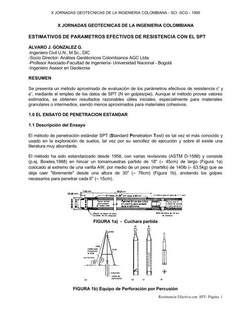
El método ha sido estandarizado desde 1958, con varias revisiones (ASTM D-1586) y consiste
(p.ej. Bowles,1988) en hincar un tomamuestras partido de 18" (≈ 45cm) de largo (Figura 1a)
colocado al extremo de una varilla AW, por medio de un peso (martillo) de 140lb (≈ 63.5kg) que se
deja caer "libremente" desde una altura de 30" (≈ 76cm) (Figura 1b), anotando los golpes
necesarios para penetrar cada 6" (≈ 15cm).
FIGURA 1a) - Cuchara partida
FIGURA 1b) Equipo de Perforación por Percusión
Resistencia Efectiva con SPT- Página 1

X JORNADAS GEOTECNICAS DE LA INGENIERIA COLOMBIANA - SCI -SCG - 1999
El valor normalizado de penetración N es para 12" (1 pie ≈ 30cm), se expresa en golpes/pie y es la
suma de los dos últimos valores registrados. El ensayo se dice que muestra "rechazo" si: (a) N es
mayor de 50 golpes/15cm, (b) N es igual a 100golpes/pie o (c) No hay avance luego de 10 golpes.
Aunque se denomina "estándar", el ensayo tiene muchas variantes y fuentes de diferencia, en
especial a la energía que llega al tomamuestras, entre las cuales sobresalen (Bowles, 1988):
1) Equipos producidos por diferentes fabricantes
2) Diferentes configuraciones del martillo de hinca, de las cuales tres son las más comunes (Figura
2): (a) el antiguo de pesa con varilla de guía interna, (b) el martillo anular ("donut") y (c) el de
seguridad
3) La forma de control de la altura de caída: (a) si es manual, cómo se controle la caida y (b) si es
con la manila en la polea del equipo depende de: el diámetro y condición de la manila, el
diámetro y condición de la polea, del número de vueltas de la manila en la polea y de la altura
real de caída de la pesa.
4) Si hay o no revestimiento interno en el tomamuestras, el cual normalmente no se usa.
5) La cercanía del revestimiento externo al sitio de ensayo, el cual debe ser estar alejado.
6) La longitud de la varilla desde el sitio de golpe y el tomamuestras.
7) El diámetro de la perforación
8) La presión de confinamiento efectiva al tomamuestras, la cual depende del esfuerzo vertical
efectivo en el sitio del ensayo.
Para casi todas estas variantes hay factores de corrección a la energía teórica de referencia Er y el
valor de N de campo debe corregirse de la siguiente forma (Bowles,1988):
Ncrr = N × Cn × η1 × η2 × η3 × η4 (1)
En la cual Ncrr = valor de N corregido
N = valor de N de campo
Cn = factor de corrección por confinamiento efectivo
η1 = factor por energía del martillo (0.45 ≤ η1 ≤ 1)
η2 = factor por longitud de la varilla (0.75 ≤ η2 ≤ 1)
η3 = factor por revestimiento interno de tomamuestras (0.8 ≤ η3 ≤ 1)
η4 = factor por diámetro de la perforación ( > 1 para D> 5'", = 1.15 para D=8")
Para efectos de este artículo se considerará que η2 = η3 = η4 = 1 y solamente se tendrán en
cuenta los factores η1 y Cn.
1.2 Corrección por Energía (h1)
Se considera que el valor de N es inversamente proporcional a la energía efectiva aplicada al
martillo y entonces, para obtener un valor de Ne1 a una energía dada "e1", sabiendo su valor Ne2 a
otra energia "e2" se aplica sencillamente la relación:
1.3 Corrección por Confinamiento (Cn)
Ne1 = Ne2 × (e2/e1) (2)
Este factor ha sido identificado desde hace tiempo (Gibbs y Holtz, 1957) y se hace por medio del
factor Cn de forma tal que:
Resistencia Efectiva con SPT- Página 2

X JORNADAS GEOTECNICAS DE LA INGENIERIA COLOMBIANA - SCI -SCG - 1999
Ncorr = N1 = Cn × N (3)
y se ha estandarizado a un esfuerzo vertical de referencia σvr’ = 1 kg/cm2 ≈ 1 atmósfera = pa ,
como función del parámetro Rs, definido por:
Rs = σv’/pa
Existen numerosas propuestas, entre las que se destacan las siguientes (Figura 2) :
Peck Cn = log(20/Rs)/log(20) (5a)
Seed Cn = 1- 1.25log(Rs) (5b)
Meyerhof-Ishihara Cn = 1.7/(0.7+Rs) (5c)
Liao-Whitman Cn = (1/Rs) 0.5
Skempton Cn = 2/(1+Rs) (5e)
Seed-Idriss Cn = 1- K*log Rs (5f)
(Marcuson) (K=1.41 para Rs

X JORNADAS GEOTECNICAS DE LA INGENIERIA COLOMBIANA - SCI -SCG - 1999
que por defecto las que más se apartan son las de Peck para Rs 1.
Además para algunas de ellas Cn puede llegar a Cn < 0, en especial para las siguientes:
Formulación Valor de Rs para Cn=0
Peck Rs > 20
Seed Rs > 6.31
Seed-Idriss Rs > 12.22
González (logartimo) Rs > 10
[S(Cn/Cn prom-1) 2 ] 0.5
100
10
1
0.1
0.01
Peck
Seed
CORRECCION DE SPT
VALORES DE Cn EN N1=Cn*N
Meyerhof-
Ishihara
Liao-Whitman
Skempton
Seed-Idriss
(Marcuson)
(0.1-1.0)Pa (1.0-5.0)Pa (5.0-10.0)Pa
(0.1-5.0)Pa (0.1-10.0)Pa Suma (0.1-1.0-5.0-10.0)
Figura 3 - Desviaciones del Promedio para Diferentes Formulaciones de Cn
Observando la raíz del cuadrado de las desviaciones para todos los intervalos (Figura 3) se
comprueba lo anterior y además se puede adicionar que las formulaciones que menos se apartan
del promedio son, en su orden, las siguientes:
a) Seed-Idriss (Marcuson)
b) Meyerhof - Ishihara
c) Schmertmann
d) Skempton
Usualmente, combinando tanto las correcciones de energía como de confinamiento el valor de N
se suele expresar como N1e. En forma inicial se considera que para martillo anular e = 45% y para
martillo de seguridad e = 70%-100%. En Estados Unidos es usual considerar que e = 60% es un
valor representativo mientras que para Japón el valor representativo puede ser e = 72%. Para
Logaritmo
Schmertmann
Resistencia Efectiva con SPT- Página 4

X JORNADAS GEOTECNICAS DE LA INGENIERIA COLOMBIANA - SCI -SCG - 1999
Colombia y, salvo mediciones al respecto (p.ej. Villafañe et al, 1997), se debe tomar,
conservativamente, e = 45%.
2.0 CORRELACIONES ENTRE N Y RESISTENCIA EFECTIVA DE LOS SUELOS
Existen numerosas correlaciones entre N y φ', pero, antes de mencionar algunas de ellas, es
conveniente discutir cual valor de φ' es el que se está obteniendo.
Dado que la mayor parte de estas correlaciones fueron obtenidas con materiales granulares, para
los cuales usualmente c' = 0, lo que realmente se obtiene es la relacion entre esfuerzos cortantes y
esfuerzos normales efectivos, es decir (Figura 4):
φ' SPT = φ'eq = arctan (τ /σ' ) (6)
t
c’
F’ ’ y F’ F
’ eq
f ’ eq
f ‘
Figura 4 - Angulo de fricción real ( f ' ) y equivalente (f 'eq )
Con lo anterior, algunas de las relaciones entre φ'eq y N1, son las siguientes:
Peck φ'eq = 28.5 + 0.25×N145 (7a)
Peck, Hanson y Thornburn φ'eq = 26.25 × (2 - exp(-N145 / 62) (7b)
Kishida φ'eq = 15 +(20 × N172) 0.5
Schmertmann φ'eq’ = arctan[(N160 / 32.5) 0.34
] (7d)
JNR φeq’ = 27 + 0.30 × N172 (7e)
JRB φeq’ = 15 + (15 × N172) 0.5
Estas relaciones, para su uso en Colombia, se deben transformar a una energia e = 45% con el
siguiente resultado:
Peck φ'eq = 28.5 + 0.25×N145 (7a)
Peck, Hanson y Thornburn φ'eq = 26.25 × (2 - exp(-N145 / 62) (7b)
s’
(7c)
(7f)
Resistencia Efectiva con SPT- Página 5

X JORNADAS GEOTECNICAS DE LA INGENIERIA COLOMBIANA - SCI -SCG - 1999
Kishida φ'eq = 15 +(12.5 × N145) 0.5
Schmertmann φ'eq’ = arctan[(N145 / 43.3) 0.34
] (8d)
Japan National Railway (JNR) φeq’ = 27 + 0.1875 × N145 (8e)
Japan Road Bureau (JRB) φeq’ = 15 + (9.375 × N145) 0.5
F'eq (°)
60
50
40
30
20
10
0
RESISTENCIA DE SPT- RELACIONES N1-F 'eq
0 10 20 30 40 50 60 70 80 90 100
N1)45 - golpes/pie
Peck Peck et al Kishida Schmertmann JNR JRB PROMEDIO
Figura 5 - Variacion de f 'eq con N1
La variación de φeq’ con N145) se presenta en la Figura 5, de la cual puede deducirse que la
relación que más se aparta del promedio por exceso es la de Schmertmann, lo cual también se
comprueba en la Figura 6, y por defecto la de JRB.
[S(F'eq/F'eq prom-1) 2 ] 0.5
2.5
2.0
1.5
1.0
0.5
0.0
Peck
RESISTENCIA DE SPT - RELACIONES N1-F 'eq
Peck,Ha
nson. et
al
Kishida
Schmert
mann
JNR
(8c)
(8f)
N1=0 a 50 N1=50 a 100 N1=0 a 100 SUMA (0-50-100)
Figura 6 - Desviaciones del Promedio para Diferentes Formulaciones de F 'eq
JRB
Resistencia Efectiva con SPT- Página 6

X JORNADAS GEOTECNICAS DE LA INGENIERIA COLOMBIANA - SCI -SCG - 1999
En la Figura 6, de variación de la raíz del cuadrado de las desviaciones para todos los intervalos, se
puede adicionar que las formulaciones que menos se apartan del promedio son, en su orden, las
siguientes:
a) Kishida b) Peck et al. c) Peck
3.0 RESISTENCIA EFECTIVA APROXIMADA CON SPT
3.1 Procedimiento
El procedimiento para obtener valores aproximados de valores efectivos de resistencia c' y φ’ con
SPT es el siguiente, teniendo en cuenta todo lo expuesto anteriormente:
a) Obtener el valor de N (golpes/pie) en campo, con la profundidad respectiva e identificar al tipo de
suelo en el cual se hizo el ensayo.
b) Colocar al ensayo la profundidad media entre las dos lecturas de golpes que se usen
c) Obtener o estimar el valor del peso unitario total de la muestra, preferentemente en el sitio. Esta
se puede obtener de la muestra de la cuchara perdida, pero corrigiendo el área por la
compresión que sufre la muestra al entrar al muestreador.
d) Obtener lo más fiablemente posible la posición del nivel piezómetrico
e) Calcular el valor de los esfuerzos totales (σ), la presión de poros (uw) y los esfuerzos efectivos
(σ’ = σ - uw) para toda la columna de ensayo. Hay que tener en cuenta que el material puede
estar saturado y la presión de poros puede ser negativa hasta la altura de capilaridad.
f) El valor de N45 para Colombia se corrige por confinamiento con la formulación de Cn de Seed-
Idriss (Marcuson), Fórmula (5f), teniendo cuidado que Cn ≤ 2.
g) Se obtiene el valor de φeq’ con la fórmula de Kishida (8c).
h) Se calcula el valor de τ = σ’ × tan(φeq’)
i) Se agrupan los valores de τ y σ’ por tipos de materiales
j) Se hace la regresión τ vs σ' para cada tipo de material y se obtienen c' y tanφ’. Si en la regresión
resulta c' < 0, se obliga a la regresión a pasar por cero.
k) Se puede obtener el φ’ mínimo de cada material haciendo φ’ mínimo = φeq’ mínimo
k) Se colocan los resultados en un diagrama c' - tanφ' y si son materiales del mismo origen
geológico, los puntos nomalmente se alinean en forma aproximada.
Este procedimiento es muy fácilmente desarrolable en una hoja electrónica de cálculo (LOTUS,
QUATTRO o EXCEL).
3.2 Limitaciones
El método indudablemente es aproximado y es útil para estimativos iniciales, pero, en lo posible,
debe siempre ser comprobado con otros ensayos preferentemente de laboratorio (corte directo,
triaxial, etc), pues tiene las siguientes importantes limitaciones.
1) El resultado normalmente, pero no siempre, es conservativo (valores de c' y tanφ’ menores que
los reales)
2) El método tiende a subestimar el valor de c', especialmente para materiales arcillosos
cohesivos.
Resistencia Efectiva con SPT- Página 7

X JORNADAS GEOTECNICAS DE LA INGENIERIA COLOMBIANA - SCI -SCG - 1999
3) En materiales granulares pueden resultar valores de c' irreales que son aproximación a una
posible envolvente curva (por ejemplo del tipo τ = A σ’ b )
4) El resultado depende de los valores de σ’, por lo tanto una sobreestimación de los valores de σ’
dará valores de c' y tanφ’ inferiores y una subestimación de σ’, valores superiores. Esto
involucra los valores usados de pesos unitarios, profundidades y presiones de poros.
5) Se ha asumido conservativamente que en Colombia la energía del SPT normalmente es 45%,
pero si se hacen calibraciones del equipo usado (p.ej. Villafañe et al, 1997), se debe usar la
energía calibrada.
3.3 Ejemplo
Se presenta un ejemplo de los valores obtenidos de 8 perforaciones realizadas en un tramo de la
vía Anserma-Riosucio, en las cuales se presentaron 14 materiales, de los cuales se dedujeron
parámetros efectivos aproximados para 11 de ellos con el siguiente resultado (Tabla 1):
TABLA 1
CARRETERA ANSERMA
Ensayo de Penetración Estandar (SPT)
Parámetros de Resistencia al Corte Deducidos
f ' prm c' prm f ' mín
SUELO
(°) (t/m2) (°)
1 Relleno heterogéneo 14.144 1.9236 26.373
2 Limo arcilloso amarillento 29.485 0.2172 34.454
3 Arena limosa amarillenta 29.234 0.1948 26.724
4 Arena limosa gris verdosa 38.866 0.0000 34.700
5 Limo arenoso carmelito 39.850 0.0000 34.551
6 Limo arenoso habano 28.066 0.1718 22.766
7 Limo arcilloso habano 28.634 0.9344 31.136
8 Arena fina algo limosa 42.014 0.0000 31.832
9 Arena con gravas 38.184 0.0000 34.369
10 Arcilla limosa habana 24.940 0.4592 28.328
14 Arena compacta habana 50.327 0.0000 48.943
Pr Promedio suelos 34.317 0.3251 33.320
φ' prm: Angulo de fricción efectivo promedio.
c' prm: Intercepto de cohesión efectivo promedio.
φ' mín: Angulo de fricción efectivo mínimo.
c' mín: Intercepto de cohesión efectivo mínimo = 0.0
Como puede apreciarse, la tabla de resultados presenta valores relativamente lógicos para la
descripción de los materiales y en la Figura 7 se aprecia que la relación entre c' y tanφ' es inversa y
aproximadamente lineal. En las Figuras 8a a 8d se presentan los diagramas τ vs σ' para 4 de los
11 materiales estudiados, en los cuales pueden apreciarse los datos y dispersiones típicas.
Resistencia Efectiva con SPT- Página 8

COHESION EFECTIVA
(ton/m2)
2.00
1.50
1.00
0.50
0.00
ESFUERZO CORTANTE (ton/m2)
X JORNADAS GEOTECNICAS DE LA INGENIERIA COLOMBIANA - SCI -SCG - 1999
CARRETERA ANSERMA - RESISTENCIA EFECTIVA DE SPT
1
10
7
632
Pr
94 5 8
0.00 0.10 0.20 0.30 0.40 0.50 0.60 0.70 0.80 0.90 1.00 1.10 1.20 1.30
6
5
4
3
2
1
0
TANGENTE DE ANGULO DE FRICCION EFECTIVO
Figura 7 - Relación Típica c' - tanf '
CARRETERA ANSERMA - SPT - RELLENO (1)
0 1 2 3 4 5 6 7 8 9
ESFUERZO NORMAL EFECTIVO (ton/m2)
C'=1.92 PHI'=14.14° "Phi' min =26.37°"
Figura 8a - Suelo 1 - Relleno
14
Resistencia Efectiva con SPT- Página 9

ESFUERZO CORTANTE (ton/m2)
ESFUERZO CORTANTE (ton/m2)
6.00
5.00
4.00
3.00
2.00
1.00
0.00
6.00
5.00
4.00
3.00
2.00
1.00
0.00
X JORNADAS GEOTECNICAS DE LA INGENIERIA COLOMBIANA - SCI -SCG - 1999
CARRETERA ANSERMA - SPT - ARCILLA LIMOSA (10)
0.00 1.00 2.00 3.00 4.00 5.00 6.00 7.00 8.00 9.00
ESFUERZO NORMAL EFECTIVO (ton/m2)
C='0.46 PHI'=24.94° PHI'mín=28.33°
Figura 8b - Suelo 10 - Arcilla limosa
CARRETERA ANSERMA -SPT - LIMO ARENOSO HABANO (6)
0.00 1.00 2.00 3.00 4.00 5.00 6.00 7.00 8.00 9.00
ESFUERZO NORMAL EFECTIVO (ton/m2)
C'=0.17 PHI'=28.07° PHI'mín=22.77°
Figura 8c - Suelo 6 - Limo arenoso habano
Resistencia Efectiva con SPT- Página 10

ESFUERZO CORTANTE (ton/m2)
X JORNADAS GEOTECNICAS DE LA INGENIERIA COLOMBIANA - SCI -SCG - 1999
14.00
12.00
10.00
8.00
6.00
4.00
2.00
0.00
AGRADECIMIENTOS
CARRETERA ANSERMA -SPT - ARENA CON GRAVAS (9)
0.00 2.00 4.00 6.00 8.00 10.00 12.00 14.00 16.00 18.00 20.00
ESFUERZO NORMAL EFECTIVO (ton/m2)
C'=0.0 PHI'=38.18° PHI'mín=35.37°
Figura 8d - Suelo 9 - Arena con Gravas
El Autor agradece al Departamento de Ingeniería Civil de la Universidad Javeriana el permiso para
publicar resultados del SPT.
REFERENCIAS
BOWLES, J.E. (1988).- Foundation Analysis and Design.- 4rd. Ed. - 1004 pp.- McGraw-Hill Book
Co.
GIBBS, H.J.; HOLTZ, W.G. (1957) - Research on Determining the Desnsity of Sands by Spoon
Penetration Testing - Proc. IV ICSMFE - London - Vol 1. pp. 35-39
ISHIHARA. K. (1989).- Dinámica Aplicada a la Estabilidad de Taludes- 206 pp.- Sociedad
Colombiana de Geotecnia - Univ. Nacional, Bogotá
JSCE (1984).- Earthquake Resistant Design for Civil Engineering Structures in Japan - Japanese
Society of Civil Engineers, Tokyo
LIAO, S.S.C; WHITMAN, R.V. (1986).- Overburden Correction Factors for SPT in Sand - JGED -
ASCE - Vol 112 No. 3, pp. 373-377.
MEYERHOF, G.G. (1957).- Discussion on Sand Density by Spoon Penetration - Proc. IV ICSMFE -
London - Vol 3. p. 110
Resistencia Efectiva con SPT- Página 11

X JORNADAS GEOTECNICAS DE LA INGENIERIA COLOMBIANA - SCI -SCG - 1999
PECK, R.B.; HANSON, W.E.; THORNBURN, (1953).- Foundation Engineering - John Wiley
POULOS, H.G.; DAVIS, E.H. (1980).- Pile Foundation Analysis and Design - 397 pp.- John Wiley &
Sons. Inc, NY
SCHMERTMANN, J.H. (1975) - Measurement of In-situ Shear Strength - Proc ASCE Specialty
Conf. on In Situ Measurement of Soil Properties - Raleigh- Vol. 2
SEED, H.B.; IDRISS, I.M. (1970).- Soil Moduli and Damping Factors for Dynamic Response
Analyses"- Report EERC 70-10- University of California- Berkeley.
SKEMPTON, A.W. (1986).- Standard Penetration Tests Procedures and the Effects in Sands of
Overburden Pressure, relatiove Density, Partricle Size, Ageing and Overconsolidation-
Geotechnique, Vol. 36, No.3 pp. 425-447
TERZAGHI,K.; PECK,R.B.(1948).- Soil Mechanics in Engineering Practice.- John Wiley and Sons
TERZAGHI,K.; PECK,R.B.; MESRI, G. (1996).- Soil Mechanics in Engineering Practice.- 3rd.
Edition- John Wiley and Sons.
VILLAFAÑE, G. et AL (1997).- IX Jornadas Geotécnicas - SCI
Resistencia Efectiva con SPT- Página 12