

Sesión # 6 Cálculo Integral Sumas de Riemann
Sesión # 6 Cálculo Integral Sumas de Riemann
Sesión # 6 Cálculo Integral Sumas de Riemann

You also want an ePaper? Increase the reach of your titles
YUMPU automatically turns print PDFs into web optimized ePapers that Google loves.
><br />
><br />
><br />
<strong>Sesión</strong> # 6<br />
<strong>Cálculo</strong> <strong>Integral</strong><br />
Dr. Il<strong>de</strong>brando Pérez Reyes<br />
En cuanto a cálculo integral MAPLE pue<strong>de</strong> cubrir muy bien casi todo el temario. Al igual que antes hay<br />
comandos para realizar cálculos <strong>de</strong> manera directa y comandos para realizar operaciones paso a paso.<br />
<strong>Sumas</strong> <strong>de</strong> <strong>Riemann</strong><br />
Cómo ya se ha <strong>de</strong> suponer las sumas <strong>de</strong> <strong>Riemann</strong> sirven para el cálculo aproximado <strong>de</strong> áreas que no<br />
pue<strong>de</strong>n ser calculadas a través <strong>de</strong> las fórmulas ya establecidas <strong>de</strong> geometría. Las sumas <strong>de</strong> <strong>Riemann</strong><br />
se <strong>de</strong>finen como<br />
en don<strong>de</strong> la función representa la función que genera una curva. El área bajo la curva se calcula con<br />
las sumas <strong>de</strong> <strong>Riemann</strong>. representa el tamaño <strong>de</strong> las particiones. representa un punto en cada<br />
partición.<br />
Para calcular las sumas <strong>de</strong> <strong>Riemann</strong>, se carga la paquetería <strong>de</strong> Calculus1,<br />
restart;<br />
with(Stu<strong>de</strong>nt[Calculus1]):<br />
Consi<strong>de</strong>remos ahora la función<br />
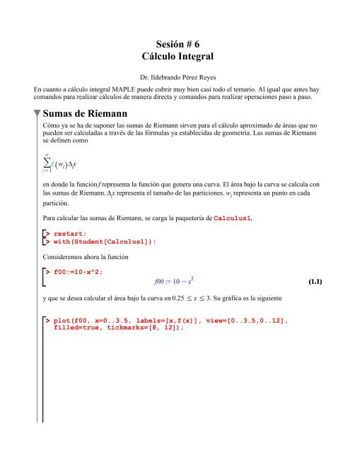
f00:=10-x^2;<br />
y que se <strong>de</strong>sea calcular el área bajo la curva en . Su gráfica es la siguiente<br />
plot(f00, x=0..3.5, labels=[x,f(x)], view=[0..3.5,0..12],<br />
filled=true, tickmarks=[8, 12]);<br />
(1.1)
f x<br />
12<br />
11<br />
10<br />
9<br />
8<br />
7<br />
6<br />
5<br />
4<br />
3<br />
2<br />
1<br />
0<br />
0 1 2 3<br />
x<br />
. Y a<strong>de</strong>más,<br />
. Para implementar la suma <strong>de</strong> <strong>Riemann</strong> <strong>de</strong> acuerdo con la fórmula anterior se tien<br />
Sumaf00:= eval(f00,x=0.5)*(1-0.25) + eval(f00,x=1.25)*(1.5-1) +<br />
eval(f00,x=1.75)*(1.75-1.5) + eval(f00,x=2)*(2.25-1.75) + eval<br />
(f00,x=2.75)*(3-2.25);<br />
Que es precisamente la respuesta <strong>de</strong>l libro.<br />
Par el caso <strong>de</strong>l comando <strong>de</strong> MAPLE, ofrece 6 diferentes opciones:<br />
Left,<br />
Right,<br />
Lower,<br />
Upper,<br />
Midpoint.<br />
(1.2)
En don<strong>de</strong> cada uno <strong>de</strong> ellos correspon<strong>de</strong> a la manera o al lugar en don<strong>de</strong> encuentran ubicados los<br />
puntos . A continuación se prueban cada uno <strong>de</strong> los métodos para la misma función<br />
><br />
><br />
<strong>Riemann</strong>Sum(f00, x=0.25..3.0, partition=[0.25,1,1.5,1.75,2.25,<br />
3], method = left, output = plot);<br />
10<br />
8<br />
6<br />
4<br />
2<br />
0<br />
A left <strong>Riemann</strong> sum approximation of<br />
1 2 3<br />
x<br />
3.0<br />
0.25<br />
f x dx, where f x = 10 Kx 2<br />
and the partition is uniform. The approximate value of the integral is<br />
21.062500. Number of subintervals used: 5.<br />
<strong>Riemann</strong>Sum(f00, x=0.25..3.0, partition=[0.25,1,1.5,1.75,2.25,<br />
3], method = right, output = plot);
10<br />
8<br />
6<br />
4<br />
2<br />
0<br />
1 2 3<br />
x<br />
A right <strong>Riemann</strong> sum approximation of<br />
3.0<br />
0.25<br />
f x dx, where<br />
f x = 10 Kx 2 and the partition is uniform. The approximate value of the<br />
integral is 15.578125. Number of subintervals used: 5.<br />
<strong>Riemann</strong>Sum(f00, x=0.25..3.0, partition=[0.25,1,1.5,1.75,2.25,<br />
3], method = lower, output = plot);
10<br />
8<br />
6<br />
4<br />
2<br />
0<br />
1 2 3<br />
x<br />
A lower <strong>Riemann</strong> sum approximation of<br />
3.0<br />
0.25<br />
f x dx, where<br />
f x = 10 Kx 2 and the partition is uniform. The approximate value of the<br />
integral is 15.578125. Number of subintervals used: 5.<br />
<strong>Riemann</strong>Sum(f00, x=0.25..3.0, partition=[0.25,1,1.5,1.75,2.25,<br />
3], method = upper, output = plot);
10<br />
8<br />
6<br />
4<br />
2<br />
0<br />
1 2 3<br />
x<br />
An upper <strong>Riemann</strong> sum approximation of<br />
3.0<br />
0.25<br />
f x dx, where<br />
f x = 10 Kx 2 and the partition is uniform. The approximate value of the<br />
integral is 21.062500. Number of subintervals used: 5.<br />
<strong>Riemann</strong>Sum(f00, x=0.25..3.0, partition=[0.25,1,1.5,1.75,2.25,<br />
3], method = midpoint, output = plot);
><br />
><br />
10<br />
8<br />
6<br />
4<br />
2<br />
0<br />
1 2 3<br />
x<br />
A midpoint <strong>Riemann</strong> sum approximation of<br />
3.0<br />
0.25<br />
f x dx, where<br />
f x = 10 Kx 2 and the partition is uniform. The approximate value of the<br />
integral is 18.59765625. Number of subintervals used: 5.<br />
Y como pue<strong>de</strong> verse ninguno <strong>de</strong> los métodos arroja unresultado que encaje con el <strong>de</strong>l libro. Por<br />
comparación con el EJEMPLO ILUSTRATIVO 1, <strong>de</strong> la sección 4.5 <strong>de</strong> Leithold se compren<strong>de</strong><br />
porque no encajan los resultados.<br />
También es posible elaborar un programa para que lo haga automáticamente. Esto se pue<strong>de</strong> hacer con<br />
un procedure<br />
funcion:= f00;<br />
x00:= 0.25:<br />
x11:= 1.0:<br />
x22:= 1.5:<br />
x33:= 1.75:<br />
x44:= 2.25:<br />
x55:= 3:<br />
x66:= 0:<br />
w11:= 0.5:<br />
w22:= 1.25:<br />
w33:= 1.75:<br />
w44:= 2:<br />
(1.3)
><br />
><br />
><br />
><br />
><br />
><br />
w55:= 2.75:<br />
w66:= 0:<br />
#PARA 4<br />
PARTICIONES#############################################<br />
SumaDe<strong>Riemann</strong>4p:= proc(x0,x1,x2,x3,x4,x5,x6, w1,w2,w3,w4,w5,w6,<br />
funcion1)<br />
<strong>de</strong>scription "Suma <strong>de</strong> <strong>Riemann</strong> para 4<br />
particiones";<br />
eval(funcion1,x=w1)*(x1-x0) + eval(funcion1,x=<br />
w2)*(x2-x1) + eval(funcion1,x=w3)*(x3-x2) + eval(funcion1,x=w4)<br />
* (x4-x3)<br />
end proc;<br />
#PARA 5<br />
PARTICIONES#############################################<br />
SumaDe<strong>Riemann</strong>5p:= proc(x0,x1,x2,x3,x4,x5,x6, w1,w2,w3,w4,w5,w6,<br />
funcion1)<br />
<strong>de</strong>scription "Suma <strong>de</strong> <strong>Riemann</strong> para 5<br />
particiones";<br />
eval(funcion1,x=w1)*(x1-x0) + eval(funcion1,x=<br />
w2)*(x2-x1) + eval(funcion1,x=w3)*(x3-x2) + eval(funcion1,x=w4)<br />
* (x4-x3) + eval(funcion1,x=w5)*(x5-x4)<br />
end proc;<br />
#PARA 6<br />
PARTICIONES#############################################<br />
SumaDe<strong>Riemann</strong>6p:= proc(x0,x1,x2,x3,x4,x5,x6, w1,w2,w3,w4,w5,w6,<br />
funcion1)<br />
<strong>de</strong>scription "Suma <strong>de</strong> <strong>Riemann</strong> para 6<br />
particiones";<br />
eval(funcion1,x=w1)*(x1-x0) + eval(funcion1,x=<br />
w2)*(x2-x1) + eval(funcion1,x=w3)*(x3-x2) + eval(funcion1,x=w4)<br />
* (x4-x3) + eval(funcion1,x=w5)*(x5-x4) + eval<br />
(funcion1,x=w6)*(x6-x5)<br />
end proc;<br />
(1.4)<br />
(1.5)<br />
(1.6)
><br />
><br />
><br />
><br />
><br />
><br />
><br />
#AHORA SE PONEN<br />
APRUEBA#############################################<br />
SumaDe<strong>Riemann</strong>4p(x00,x11,x22,x33,x44,x55,x66, w11,w22,w33,w44,<br />
w55,w66,funcion);<br />
16.265625<br />
SumaDe<strong>Riemann</strong>5p(x00,x11,x22,x33,x44,x55,x66, w11,w22,w33,w44,<br />
w55,w66,funcion);<br />
18.093750<br />
Calculemos ahora el siguiente ejercicio:<br />
(1.7)<br />
(1.8)<br />
Obviamente, son 4 particiones y se pue<strong>de</strong> resolver fácilmente con el procedure SumaDe<strong>Riemann</strong>4p<br />
funcion:= x^2;<br />
(1.9)<br />
x00:= 0:<br />
x11:= 0.5:<br />
x22:= 1.25:<br />
x33:= 2.25:<br />
x44:= 3:<br />
w11:= 0.25:<br />
w22:= 1.:<br />
w33:= 1.5:<br />
w44:= 2.5:<br />
SumaDe<strong>Riemann</strong>4p(x00,x11,x22,x33,x44,x55,x66, w11,w22,w33,w44,<br />
w55,w66,funcion);#QUE CONCUERDA PERFECTAMENTE!!!!!<br />
7.71875<br />
(1.10)<br />
plot(x^2, x=0..3.5, labels=[x,f(x)], view=[0..3,0..10], filled=<br />
true, tickmarks=[8, 12]);
f x<br />
10<br />
9<br />
8<br />
7<br />
6<br />
5<br />
4<br />
3<br />
2<br />
1<br />
0<br />
0 1 2 3<br />
x<br />
Ahora, resolvamos el mismo problema pero con el método <strong>de</strong>l punto medio<br />
<strong>Riemann</strong>Sum(x^2, x=0.25..3.0, partition=[0,0.5,1.25,2.25,3],<br />
method = midpoint, output = plot, boxoptions=[filled=[color=<br />
pink,transparency=.7]]);
><br />
><br />
8<br />
6<br />
4<br />
2<br />
0<br />
A midpoint <strong>Riemann</strong> sum approximation of<br />
1 2 3<br />
x<br />
3.0<br />
0.25<br />
f x dx, where f x = x 2<br />
and the partition is uniform. The approximate value of the integral is<br />
8.832031250. Number of subintervals used: 5.<br />
<strong>Integral</strong>es <strong>de</strong>finidas e in<strong>de</strong>finidas<br />
Las integrales <strong>de</strong>finidas son <strong>de</strong> gran importancia no sólo en matemáticas sino también en física e<br />
ingeniería <strong>de</strong>bido a sus usos para calcular áreas , volúmenes, etc.. En MAPLE el comando para<br />
resolver este tipo <strong>de</strong> integrales es simple: int(función,variable=límites);<br />
Veamos el siguiente ejemplo:<br />
f01:= x^2;<br />
que se va a integrar entre el intervalo entonces<br />
int(f01,x=0..3);<br />
Considérese ahora la integral <strong>de</strong> en el intervalo<br />
int(x,x=0..3);<br />
9<br />
(2.1)<br />
(2.2)<br />
(2.3)
><br />
><br />
9<br />
2<br />
plot(x, x=0..3., labels=[x,f(x)], view=[0..3,0..3], filled=<br />
true, tickmarks=[8, 12]);<br />
f x<br />
3<br />
2<br />
1<br />
0<br />
0 1 2 3<br />
x<br />
Considérese el siguiente ejemplo. en el intervalo<br />
int(sqrt(9-x^2),x=-3..3);<br />
evalf(int(sqrt(9-x^2),x=-3..3));<br />
(2.3)<br />
14.13716694<br />
(2.4)<br />
plot(sqrt(9-x^2), x=-4..4., labels=[x,f(x)], view=[-4..4,0..6],<br />
filled=true, tickmarks=[8, 12]);
><br />
f x<br />
6<br />
5<br />
4<br />
3<br />
2<br />
1<br />
0 1 2<br />
x<br />
3 4<br />
Considérese el siguiente ejemplo. en el intervalo<br />
int(sin(x),x=0..2*Pi);<br />
0<br />
plot(sin(x),x=0..2*Pi, labels=[x,f(x)], view=[0..2*Pi,-1..1],<br />
filled=true, tickmarks=[8, 12]);<br />
(2.5)
><br />
><br />
><br />
f x<br />
1<br />
0<br />
Así con otros ejercicios:<br />
f02:= sqrt(5+4*x-x^2);<br />
int(f02,x=-1..5);<br />
f03:= 6-abs(x-2);<br />
int(f03,x=0..8);<br />
1 2 3 4 5 6<br />
x<br />
28<br />
En cuanto a integrales <strong>de</strong>finidas hay <strong>de</strong> muchos tipos y la sintaxis es mucho más simple. Basta con<br />
quitar los límites. Por ejemplo, intégrese la función<br />
(2.6)<br />
(2.7)<br />
(2.8)<br />
(2.9)
><br />
><br />
><br />
><br />
><br />
><br />
f04:= (x^2+2)/(x+1);<br />
int(f04,x);<br />
f05:= (2-3*sin(2*x))/cos(2*x);<br />
int(f05,x);<br />
<strong>Integral</strong>es <strong>de</strong>finidas e in<strong>de</strong>finidas paso a paso<br />
Para resolver integrales paso a paso con ayuda <strong>de</strong> un asistente se carga la paquetería:<br />
with(Stu<strong>de</strong>nt[Calculus1]);<br />
y <strong>de</strong> allí se usa el comando Inttutor. considérese la función<br />
IntTutor(x^3,x);<br />
La misma integral se pue<strong>de</strong> hacer en el intervalo[0,3]<br />
IntTutor(x^3,x=0..3);<br />
(2.10)<br />
(2.11)<br />
(2.12)<br />
(2.13)<br />
(3.1)<br />
(3.2)<br />
(3.3)
Considéres una función más complicada<br />
><br />
><br />
><br />
><br />
><br />
><br />
f06:= 1/(1+exp(x));<br />
IntTutor(f06,x);<br />
y a<strong>de</strong>más se <strong>de</strong>sea ver los pasos. Entonces, se usa ShowSolution<br />
ShowSolution(IntTutor(f06,x));<br />
f07:= exp(2*x)/(exp(x)+3);<br />
=<br />
=<br />
=<br />
=<br />
=<br />
=<br />
=<br />
=<br />
=<br />
IntTutor(f07,x);<br />
ShowSolution(Int(f07,x));<br />
(3.4)<br />
(3.5)<br />
(3.6)<br />
(3.7)<br />
(3.8)
Aproximación <strong>de</strong> integrales<br />
><br />
><br />
=<br />
=<br />
=<br />
=<br />
=<br />
=<br />
=<br />
=<br />
=<br />
Las <strong>Integral</strong>es pue<strong>de</strong>n ser aproximadas gráficamente en el estilo <strong>de</strong> las sumas <strong>Riemann</strong>. En ese<br />
sentido, MAPLE provee un comando idóneo ApproximateInteTutor<br />
Considérese la siguiente función en el intervalo [0,3]<br />
f08:= x^3;<br />
ahora usemos el comando para aproximar la integral<br />
ApproximateIntTutor(f08,x=0.3);<br />
(3.9)<br />
(4.1)
Considérese la función<br />
><br />
><br />
f07;<br />
en el intervalo [0,5]<br />
ApproximateIntTutor(f07,x=0..5);<br />
30<br />
20<br />
10<br />
0 1 2 3<br />
(4.2)
160<br />
140<br />
120<br />
100<br />
80<br />
60<br />
40<br />
20<br />
0<br />
1 2 3 4 5<br />
<strong>Integral</strong>es <strong>de</strong>finidas por la regla <strong>de</strong> Simpson<br />
La regla <strong>de</strong> Simpson es un método para aproximar el valor numérico <strong>de</strong> una integral <strong>de</strong>finida.<br />
La regla <strong>de</strong> Simpson está <strong>de</strong>finida <strong>de</strong> forma aproximada en el libro <strong>de</strong> Leithold como sigue<br />
=<br />
La fórmula exacta <strong>de</strong> la regla <strong>de</strong> Simpson es<br />
=
De nueva cuenta, se necesita la paquetería Calculus1 y el comando a usar es ApproximateInt<br />
><br />
><br />
><br />
><br />
><br />
with(Stu<strong>de</strong>nt[Calculus1]);<br />
Considérese que se <strong>de</strong>sea usar la regla <strong>de</strong> Simpson para aproximar la siguiente integral<br />
Obviamente esta pue<strong>de</strong> calcularse fácilmente como sigue<br />
f09:= 1/(1+x);<br />
int(f09,x=0..1.);<br />
0.6931471806<br />
Ahora, aplicaremos la regla <strong>de</strong> Simpson con N=4<br />
ApproximateInt(f09,x=0..1., method=simpson, partition=4);<br />
0.6931545307<br />
ApproximateInt(f09,x=0..1, method=simpson, output=plot,<br />
partition=4);<br />
(5.1)<br />
(5.2)<br />
(5.3)<br />
(5.4)
><br />
><br />
><br />
0<br />
An approximation of<br />
0<br />
1<br />
x<br />
f x dx using Simpson's rule, where<br />
1<br />
f x = and the partition is uniform. The approximate value of the<br />
xC1<br />
integral is 0.6931545307. Number of subintervals used: 4.<br />
Considérese otra función<br />
f10:= exp(-x^2/2);<br />
int(f10,x=0..2);<br />
evalf(int(f10,x=0..2));<br />
1.196288013<br />
ApproximateInt(f10,x=0..2., method=simpson, partition=4);<br />
1.196281734<br />
ApproximateInt(f10,x=0..2, method=simpson, output=plot,<br />
partition=4);<br />
1<br />
(5.5)<br />
(5.6)<br />
(5.7)
0<br />
An approximation of<br />
0<br />
2<br />
1 2<br />
x<br />
f x dx using Simpson's rule, where<br />
f x = e K1<br />
2 x2<br />
and the partition is uniform. The approximate value of the<br />
integral is 1.196281734. Number of subintervals used: 4.<br />
Longitud <strong>de</strong> arco<br />
Para el cálculo <strong>de</strong> longitud <strong>de</strong> arco se usa <strong>de</strong> igual forma la paquetería <strong>de</strong> Calculus1. Esta tiene dos<br />
opciones<br />
ArcLengthTutor<br />
ArcLength<br />
with(Stu<strong>de</strong>nt[Calculus1]);<br />
(6.1)
Calcúlese entonces, la longitud <strong>de</strong> arco <strong>de</strong> la función <strong>de</strong>s<strong>de</strong> el punto (1,1) hasta el punto (8,<br />
4)<br />
><br />
><br />
><br />
><br />
f11:= x^(2/3);<br />
ArcLength(f11,x=1..4);<br />
ArcLength(f11,x=1..4.);<br />
3.367636667<br />
ArcLength(f11,x=1..4, output=integral);<br />
ArcLength(f11,x=1..4, output=plot, axes=boxed);<br />
3<br />
2<br />
1<br />
0<br />
1 2 3 4<br />
x<br />
f x g x = 1 C d<br />
dx<br />
f x<br />
2<br />
x<br />
1<br />
g s ds<br />
The arc length of f x = x 2 /3 on the interval 1, 4 . The coordinate<br />
system is Cartesian.<br />
(6.2)<br />
(6.3)<br />
(6.4)
Probemos ahora con el otro comando<br />
><br />
ArcLengthTutor(f11,x=1..4);<br />
y<br />
3<br />
2<br />
1<br />
0<br />
1 2 3 4<br />
x<br />
Superficies <strong>de</strong> revolución<br />
Para el cálculo <strong>de</strong> superficies <strong>de</strong> revolución se usa <strong>de</strong> igual forma la paquetería <strong>de</strong> Calculus1. Esta<br />
tiene dos opciones<br />
SurfaceOfRevolution<br />
SurfaceOfRevolutionTutor<br />
Definición <strong>de</strong> unsa superficie <strong>de</strong> revolución:<br />
Si una curva plana se gira alre<strong>de</strong>dor <strong>de</strong> una recta fija que está en el plano <strong>de</strong> la curva, entonces la<br />
superficie así generada se <strong>de</strong>nomina superficie <strong>de</strong> revolución. La recta fija se llama eje <strong>de</strong> la<br />
superficie <strong>de</strong> revolución, y la curva plana recibe el nombre <strong>de</strong> curva generatriz (o revolvente).
with(Stu<strong>de</strong>nt[Calculus1]);<br />
Considérese el siguiente ejemplo tomado <strong>de</strong>l libro <strong>de</strong> Leithold sección 10.6 superficies<br />
Ejemplo ilustrativo. (Leithold, Sec. 10.6 Superficies)<br />
Una esfera es generada al girar la semicircunferencia alre<strong>de</strong>dor <strong>de</strong>l eje<br />
Consi<strong>de</strong>rar que<br />
><br />
><br />
with(plots);<br />
implicitplot(y^2+z^2=2,y=-2..2,z=-2..2, view=[-1.5..1.5,0.<br />
.1.5]);<br />
(7.1)<br />
(7.1.1)
><br />
><br />
0 1<br />
y<br />
Entonces, reescribamos la expresión en términos <strong>de</strong><br />
y00:= sqrt(2-z^2);<br />
z<br />
1<br />
ahora usamos el comando SurfaceOfRevolution y calculamos el valor <strong>de</strong> la superficie <strong>de</strong><br />
revolución<br />
SurfaceOfRevolution(y00, z=-1.414..1.414);<br />
25.12894590<br />
25.12894590<br />
ahora veamos la posibilidad <strong>de</strong> ver una esfera<br />
SurfaceOfRevolution(y00, z=-1.414..1.414, output=plot, axes=<br />
frame);<br />
(7.1.2)<br />
(7.1.3)
Surface of revolution formed when f x = 2Kz 2 ,<br />
K1.414 % z % 1.414, is rotated about a horizontal axis.<br />
Un cilindro circular rectose genera a partir <strong>de</strong> la curva generatriz <strong>de</strong>l plano y su eje es el<br />
eje . Considérese que<br />
plot(4,x=-2..2);
><br />
6<br />
5<br />
4<br />
3<br />
0<br />
x<br />
1 2<br />
ahora usamos el comando SurfaceOfRevolution y calculamos el valor <strong>de</strong> la superficie <strong>de</strong><br />
revolución<br />
SurfaceOfRevolution(4, z=-2..2);<br />
SurfaceOfRevolution(4, z=-2..2.);<br />
ahora veamos la posibilidad <strong>de</strong> ver una esfera<br />
100.5309649<br />
SurfaceOfRevolution(4, z=-2..2, output=plot, axes=frame,<br />
surfaceoptions=[shading=zhue]);<br />
(7.1.4)
otro ejemplo,<br />
><br />
Surface of revolution formed when f x = 4, K2 % z % 2, is rotated<br />
about a horizontal axis.<br />
SurfaceOfRevolution(cos(x) + 1, x=0..4*Pi, output=plot);
Surface of revolution formed when f x = cos x C1, 0 % x % 4 p, is<br />
rotated about a horizontal axis.<br />
SurfaceOfRevolution(1/x*cos(x), Pi..4*Pi, output=plot, axis=<br />
vertical);
cos x<br />
Surface of revolution formed when f x =<br />
x<br />
rotated about a veritcal axis.<br />
Usemos ahora el segundo comando para abrir el asistente<br />
SurfaceOfRevolutionTutor(1+sin(x));<br />
, p % x % 4 p, is
plot(1+sin(x),x);
2<br />
1<br />
0<br />
2 2<br />
x<br />
SurfaceOfRevolutionTutor(1+sin(x), 0..Pi);
Volúmenes <strong>de</strong> revoluión<br />
><br />
><br />
><br />
><br />
><br />
with(Stu<strong>de</strong>nt[Calculus1]):<br />
VolumeOfRevolution(x^2 + 1, x=0..1);<br />
VolumeOfRevolution(x^10 + 1, x^2 + 1, x=0..1, distancefromaxis=<br />
-1);<br />
VolumeOfRevolution(sin(x) + 1, x=0..3, output=integral);<br />
Int(Pi*(sin(x)+1)^2,x=0..3);<br />
(8.1)<br />
(8.2)<br />
(8.3)<br />
(8.4)
><br />
><br />
VolumeOfRevolution(sin(x) + 1, x=2*Pi..3*Pi, output=integral,<br />
axis=vertical);<br />
VolumeOfRevolution(cos(x) + 1, x=0..4*Pi, output=plot);<br />
The solid of revolution created on 0 % x % 4 p by rotation of<br />
f x = cos x C1 about the axis y = 0.<br />
VolumeOfRevolution(cos(x) + 3, sin(x) + 2, x=0..4*Pi, output=<br />
plot);<br />
(8.4)<br />
(8.5)
The solid of revolution created on 0 % x % 4 p by rotation of<br />
f x = cos x C3 and g x = sin x C2 about the axis y = 0.<br />
VolumeOfRevolution(x^2, x=-1..1, output=plot, showregion=true);
><br />
The solid of revolution created on K1 % x % 1 by rotation of f x = x 2<br />
about the axis y = 0. The slice that is rotated is sha<strong>de</strong>d in burgundy.<br />
#############<br />
VolumeOfRevolutionTutor(1+sin(x));
VolumeOfRevolutionTutor(1+sin(x), 0..Pi);